Article
Application of Shannon Entropy in the Construction
of a Paraconsistent Model of the Atom
João Inácio da Silva Filho *
Laboratory of Applied Paraconsistent Logic, Santa Cecilia University Oswaldo Cruz Street, 288, Santos City, SP, Brazil, 11045-000
* Correspondence: [email protected]
Abstract: In this work, we present a model of the atom that is based on a nonclassical logic called paraconsistent logic (PL), which has the main property of accepting the contradiction in logical interpretations without the conclusions being annulled. The proposed model is constructed with an extension of PL called paraconsistent annotated logic with annotation of two values (PAL2v), which is associated with an interlaced bilattice of four vertices. We use the logarithmic function of the Shannon entropy H(s) to construct the paraconsistent equations and thus adapt a probabilistic model for representations in quantum physics. Through analyses of the interlaced bilattice, comparative values are obtained for some of the phenomena and effects of quantum mechanics, such as superposition of states, quantum entanglement, wave functions, and equations that determine the energy levels of the layers of an atom. At the end of this article, we use the hydrogen atom as a basis of the representation of the PAL2v model, where the values of the energy levels in six orbital layers are obtained. As an example, we present a possible method of applying the PAL2v model to the use of Raman spectroscopy signals in the detection of lubricating mineral oil quality.
Keywords: quantum information; Shannon entropy; quantum physics; paraconsistent logic; mathematics and computing
1. Introduction
The model of the atom was presented by Niels Bohr in 1913, where he proposed that electrons are particles with two kinds of motions in atoms. In the Bohr model, the electrons either move continuously around the nucleus in certain stationary orbits or discontinuously jump between these orbits [1]. Subsequently, with the advances in quantum theory, new concepts, such as the ideas of superposition of states and quantum entanglement, have been proposed. Currently, the physical state of an electron is described by a wave function and in the foundations of quantum mechanics; the wave function is a description of the random discontinuous motion of particles. Moreover, the data on the physical properties of particles are uncertain, and all of the analyses are probabilistic [1,2].
The probability density of the particle appearing in each position is proportional to the square of the modulus of its wave function at every instant. The square of the modulus of the wave function represents not only the probability of a particle being found at a certain location but also the probability of the particle being there [2][3].
In 1925, Heisenberg published results introducing the quantum concepts for particles in matrix analysis. In the matrix formulation, the instantaneous state of a quantum system encodes the probabilities of its measurable properties or “observables,” which include energy, position, momentum, and angular momentum. Observables can be either continuous (e.g., the position of a particle) or discrete (e.g., the energy of an electron bound to a hydrogen atom) [2,3].
In 1926, Schrödinger proposed a partial differential equation for the wave functions of particles, such as electrons. The state of a system at a given time is described by a complex wave function, which is also referred to as the state vector in a complex vector space, and this abstract mathematical object enables the calculation of the probabilities of outcomes of concrete experiments [3,4].
Another important consideration is that in quantum mechanics, one can never make simultaneous predictions of conjugate variables, such as position and momentum, to arbitrary precision. In 1927,
Heisenberg proposed the uncertainty principle, which shows the formal inequality relating the uncertainty of
position x and the uncertainty of momentump, as follows [3-5]:
2
x p h . (1)
The electrons may be considered (to a certain probability) to be located somewhere within a given region of space. However, their exact positions are unknown. In this condition, contours of constant probability density, which are often referred to as “clouds,” may be drawn around the nucleus of an atom to conceptualize where an electron might be located with the most probability [2][5-8]. The probability density is obtained using the square of the amplitude of the wave function, which usually involves a complex quantity. Thus, its value is derived by multiplication with the conjugate complex, as follows [6,7]:
. (2)
If the wave function is a representative of the sum of probabilities that describe a particle, then it needs to
be normalized, as follows [3][8,9]: + *( , ). ( , ) 1
− =
x t x tdx .With respect to the logic applied to quantum mechanics among various studies of quantum probabilistic logic formalism, one of the most important was developed by von Neumann in 1932 [11,12]. In his work, von Neumann assumed that each physical system is associated with a Hilbert space H (separable), with its unit vectors corresponding to possible physical states of the system. Each real “observable” random quantity is represented by a self-regulated operator A in H, whose spectrum is the set of possible values of A [12]. According to the previous works, mathematics in quantum mechanics can be considered a nonclassical probability calculation, which is supported by a nonclassical propositional logic [13,14].
1.1 Paraconsistent Logic
Nonclassical logics are created with the purpose of opposing the binary principles of classical logic, thus providing better conditions for the construction of physical–mathematical models with more approximate results. Currently, there are several types of nonclassical logics, and in general, we can consider that only those logics that are indestructible in the presence of the contradiction are paraconsistent. Therefore, a paraconsistent logic (PL) is a nonclassical logic that has, as its fundamental characteristic, the opposition to the principle of noncontradiction [15-18].
The fundamental theory of PL has been developed in the area of philosophical logic [19], and a formal framework for inconsistent theories was proposed by da Costa [15][17][19]. Further details of the logical formalization of PL, the mathematical implications, and their theorems can be found in [15], [17], and [20].
Blair and Subrahmanian [21] presented applications of PL to logical programming and extended the formalization of three-valued semantics. With this initial work, a theory was developed for possibly inconsistent logic programs using a lattice also known as Belnap’s four-valued logic [22], where the set of truth values of four-valued logic is defined as τ ={ t, f, ⊺, ⊥}, in which t, f, ⊺, and ⊥ are propositions in the language of a program, and they denote true, false, contradictory, and paracomplete, respectively. The set of truth values τ comprises a complete lattice under the ordering ≤, such that ⊥ ≤ x ≥ ⊺ for x τ = {t, f} [22,23].
1.2 Paraconsistent Annotated Logic with Annotation of Two Values
An extended form of PL, the paraconsistent annotated logic (PAL), which has an associated lattice, has been investigated and applied to several fields of science [18] [23,24]. In data analysis systems, the PAL can derive an annotation composed of two degrees of evidence from different sources of information and, in this case, is named paraconsistent annotated logic with annotation of two values– PAL2v [25,26]. The first concepts of PAL2v, which can be applied to artificial intelligence, are presented in [25].
As presented in [18], [26,27], and [28], in the application of PAL2v, the associated lattice is considered an abstract universe τ, where a negation operator allows logical interpretations to result in paraconsistent equations. In the annotation, the first degree of evidence is favorable for the proposition P and is represented by the symbol μ, and the second degree of evidence is unfavorable for the proposition P and is represented by the symbol λ. These degrees of evidence are normalized, classified as a set of real numbers, and contained in the closed interval [0,1]. The annotation assigns a logical state to the proposition P. Thus, the information in PAL2v is a paraconsistent logical signal represented by the proposition P with the subscript of the annotation as (μ, λ):P( , ) , where the annotation is composed of a pair of the degrees of favorable evidence (μ) and unfavorable evidence (λ).
The paraconsistent symbol (μ, λ) assigns a logical state to proposition P as follows [25,26]:
2 *
( , ) ( , ) = x t x t
1. If the annotation is (0, 1), then the degree of favorable evidence is minimum and the degree of unfavorable evidence is maximum, which provides a logical “false” connotation to proposition P. This paraconsistent signal defines the logical state “false” f.
2. If the annotation is (1, 0), then the degree of favorable evidence is maximum and the degree of unfavorable evidence is minimum, which provides a logical “true” connotation to proposition P. This paraconsistent signal defines the logical state “true” t.
3. If the annotation is (1, 1), then the degree of favorable evidence is maximum and the degree of unfavorable evidence is maximum, which provides a logical true and false connotation to proposition P. This paraconsistent signal defines the logical state “inconsistent” ⊺.
4. If the annotation is (0, 0), then the degree of favorable evidence is minimum and the degree of unfavorable evidence is minimum, which provides a logical false and true connotation to proposition P. This paraconsistent signal defines the logical state “paracomplete” ⊥.
Figure 1(a) shows the lattice FOUR associated with PAL and the representations of the extreme logical states in their vertices through the annotation (μ, λ) of PAL2v [25][29,30].
As discussed in [31,32], and [33], this representation of PAL2v has been recently investigated using an interlaced bilattice also known as the bilattice of Belnap [22,23][34]. A bilattice is a structure
B=B, t, k , where Bis a nonempty set, and
B
,
k and
B
,
t are both bounded lattices, that is, with bottom and top elements. In studies of bilattice, the symbols, ⊗k and ⊕k are used to denote the meet and join operations that correspond to k, respectively, and ⊗t and ⊕t are used to denote the meet and joinoperations that correspond to t, respectively. The partial order
kis intended to represent the knowledge or information order, and tis intended to represent the truth order. In other words, the knowledge order reports on how much information we have about a particular statement p, whereas the truth order reports on how confident we are that p is true or false. Interpreting xt y, we simply thereby mean that y is truer than x; in turn, we interpret xk yto mean that the evidence underlying x is subsumed by the evidence underlying y [22][34].Figure 1(b) shows the interlaced bilattice of Belnap with the ordering tand kand the representations of the extreme logical states in their four vertices, t, f, ⊺, and ⊥, which denote truth, falsity, both, and none, respectively [22,23][25].
(a) (b)
Fig. 1. Lattices associated with nonclassical logics –LPA and four-valued logic: (a) lattice FOUR associated with PAL2v and representations of the extreme logical states in their vertices through the annotation (μ, λ); (b)
interlaced bilattice of Belnap with the ordering t k and four extreme logical states represented in their vertices.
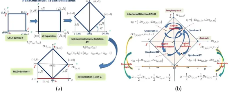
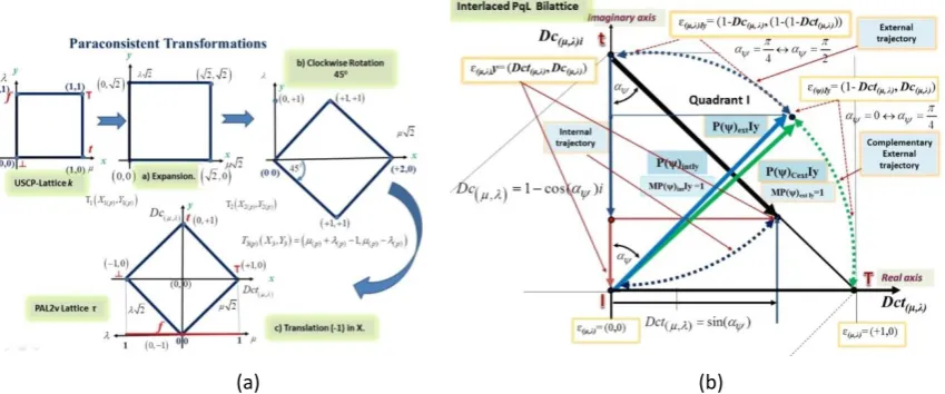
The paraconsistent equations are obtained from mathematical transformations that map the values arranged in a unitary square on the Cartesian plane (USCP) to the associated bilattice of PAL2v [25,26].
(
) (
)
2 2, 2 = 1cos − 1 sin , 1sin + 1cos
T X Y X Y X Y , where cos 1
2
=
and sin 1
2 =
; (c) translation of the −1
value from the y-axis T X Y3
(
3, 3) (
= X Y2, 2−1)
resulting in .If x is the value allocated to the x-axis of the USCP and y is the value allocated to the y-axis of the
USCP, then x=
and y=. The previously described actions create T1, T2, and T3 transformations, asdescribed in [26] and [31], which results in the following:
T X Y3
(
3, 3) (
=
− , + −1)
. (3) We denote the certainty degree (Dc) as X3 and the contradiction degree (Dct) as Y3 [26][31]:( ) 3= ,
X Dc → Certainty degree as a function of μ and λ:
Dc( , ) = − , (4) ( )
3= ,
Y Dct → Contradiction degree as a function of μ and λ:
Dct( ) , = + − 1. (5)
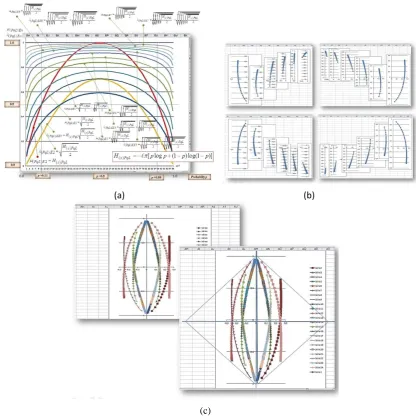
Figure 2(a) shows this mapping with the sequences of actions to obtain the equations of the paraconsistent transformations and associated bilattice of PAL2v in the degrees of certainty and contradiction in the x- and y-axes.
The maximum negative value of the degree of certainty is −1 at the vertex of the extreme logical state “false” (f) and the maximum positive value is +1 at the vertex of the extreme logical state “true” (t). For these two conditions, the value of the degree of contradiction will always be 0 .
The maximum negative value of the degree of contradiction is −1 at the vertex of the extreme logical state “paracomplete” (⊥), and the maximum positive value is +1 at the vertex of the extreme logical state “inconsistent” (⊺). For these two conditions, the value of the degree of certainty will always be 0 ( )
,
(Dc =0) [25,26]. Furthermore, PAL2v, when applied to quantum mechanics, is called paraquantum logic (PqL). In the interlaced PqL bilattice, the values are represented by a universe of complex numbers, where the degree of contradiction lies in the imaginary axis and the degree of certainty lies in the real axis, with the origin at the point equidistant from the vertices of the bilattice; therefore, in this point, the degrees of certainty and contradiction are both equal to 0 [31-33].
The paraconsistent logical state, which defines the paraquantum logical state [31], is considered the
point of intersection between the degrees of certainty (Dc( ) , ) and contradiction (Dct( , )) located in the bilattice FOUR or the PqL bilattice. Therefore, the paraquantum logical state can be expressed as follows
[25,26]:
( , )=
(
Dc( , ) ,Dct( , ) )
. (6)Through mapping, the bilattice associated with PqL becomes a lattice of values, where the equations obtained create pairs of the values ofDc( , ) andDct( ) , , which define infinite internal points of intersection.
Each internal point of intersection composed of a pair of values is a single paraquantum logical state ( , ).
The equations obtained from the transformations enable the determination of the distance between the
paraquantum logical state represented by a pair of inseparable values
(
Dc( , ),Dct( , ))
and the extreme logical states represented by the vertices of the bilattice. Given that Dc( , ) and Dct( ) , are dependent on the μ and λ values, the distance between the logical state resulting from ( , ) and one of the extreme logicalstates t, f, ⊺, or ⊥, represented by the vertices of the PqL bilattice, is dependent on the values of μ and λ considered in the physical world. If we know the paraquantum logical state ετ in any region inside the PqL
bilattice, then the values of the degrees of evidence can be calculated using the following equations [26][31]:
( ) ( ,) (,)
1 1 1
2 2 2
= + +
p Dc Dct
(7)
and
( ) ( )
( ) , ,
1 1 1
2 2 2
−
= + +
p Dc Dct
. (8)
Non-commutation exists between the degrees of evidence of the PqL and is explained by the logical negation operation denoted by the symbol. The change of position of the degrees of evidence in the
(
) (
)
3 3
,
3=
−
,
+ −
1
T X Y
x y x
y
annotation negates proposition P. Therefore, given proposition P, its logical negation P is represented by the exchange of the degrees of evidence in the annotation, as follows [31-33]:
( ) ( )
, =
, . (9) An interlaced bilattice [31][33] in addition to the negation operation expressed in Eq.(9) also enables the application of the complementation and conflation operations. The logical complementation operation in the PqL, denoted by the symbol, is an explicit complement to the unit of the degrees of evidence in the annotation. Given proposition P and its complement P, we can express the complementation operation as follows:(
,) (
1 ,1)
= − − . (10) The logical conflation operation in the PqL, denoted by the symbol‡ , is explained by the negation operation, followed by the complement to the unit of the degrees of evidence in the annotation [31]. Given proposition P and its conflation P, we can express the conflation operation as follows:
‡
(
,) (
= −1 ,1−)
. (11) For a logical–mathematical study, the interlaced bilattice associated with PqL can be divided into four quadrants [31]: (a) In Quadrant I, the degrees of certainty and contradiction are positive (there is no operator action on the annotation ( , )); (b) in Quadrant II, the degree of certainty is negative, while the degree ofcontradiction is positive (this is an action of the logical negation operator over the annotation( , )); (c) in Quadrant III, the degrees of certainty and contradiction are negative (this is an action of the logical complementation operator over the annotation ( , )); and in Quadrant IV, the degree of certainty is
positive, while the degree of contradiction is negative (this is an action of the logical conflation operator ‡ over the annotation ).
With the negation, complementation, and conflation operations only over the values of the degrees of certainty and contradiction obtained in Quadrant I, the results of the degrees of certainty and contradiction are obtained in the three other quadrants of the interlaced PqL bilattice. Therefore, given that we detect the paraquantum logical state in Quadrant I with the corresponding values of Dc( ) , and Dct( ) , , the negation operation results in a negative degree of certainty and an unchanged degree of contradiction. This results in
another paraquantum logical state in Quadrant II, which is represented by
(
−Dc( ) , ,+Dct( ) ,)
[31][33]. Similarly, the complementation operation on the values of the degrees of certainty and contradiction in Quadrant I results in negative values for both the degrees of certainty and contradiction. This result definesthe paraquantum logical state in Quadrant III, which is represented by
(
−Dc( ) , ,−Dct( ) ,)
. The conflationoperation on the values of the degrees of certainty and contradiction in Quadrant I results in positive values for the degree of certainty and negative values for the degree of contradiction. This result defines the
paraquantum logical state in Quadrant IV, which is represented by [31,32].
Figure 2(b) shows the interlaced PqL bilattice with quadrant operators and paraconsistent equations for reversible logic.
(a) (b)
Fig. 2. Sequences of mapping to obtain the paraconsistent equations and representations in the interlaced PqL bilattice: (a) sequences followed to obtain the equations of the paraconsistent transformations with counterclockwise rotation; (b) interlaced PqL bilattice with quadrant operators and paraconsistent equations
for reversible logic.
‡
(
,)
( ) ( )
1.3 Shannon Entropy
In a work by Shannon in 1948 [35], the basis of the mathematical theory of communication, or
information theory, was established. Moreover, Shannon’s work emphasizes a fundamental concept, that is,
the entropy of the information, which has become well known as the Shannon entropy H(s). The Shannon
entropy has complementary interpretations that can be either information quantity (after measurement) or
uncertainty (before measurement) in a given probability distribution [36,37]. To establish the current concept
that H(s) is a function of entropy, similar to Boltzmann’s H theorem, Shannon defined some statistical
concepts through the equation
( ) 1
log = = −
n
s i
H k pi pi, where pi is the probability of a system being in cell i of its
phase space, and k corresponds only to a certain unit of measure [36][38,39].
The equation of entropy in the case of two variables, that is, p and q (where q = 1–p), is written as follows: H( )s = −k p[ logp q+ log ]q , (12)
where p is the probability, q is its complement (1–p), and the constant k depends on the variable used [36, 37]. As can be seen in [36] and [37], to obtain the maximum unitary value of H(s) in Eq. (12), k is calculated as
log10 1 1
3.321928 log 2 log 2 0.301029995
= = = ;
k .
1.4 Rydberg’s Formula
In 1890, before Bohr introduced his model of the atom, Johannes Rydberg developed formulas describing
the wavelengths or frequencies of light in various series of related spectral lines [40]. Later, Bohr expressing
results in terms of wavenumber, not wavelength, combined these formulas. These studies resulted in the
following equation [1][40]:
2
2 2
1 1
1 1 1
= −
R Z
n n
, (13)
where
is the wavelength of the photon (wavenumber = 1/wavelength);
Zis the atomic number of the atom;
1
n is the principal quantum number of an energy level, for the atomic electron transition;
2
n is the principal quantum number of an energy level for the atomic electron transition, with n2 n1; and
R is the Rydberg's constant, calculated as
4
-1 2 3
0
1.0973731568539 8
= =
e m e
R m
h c
,
where me is the mass of the electron, eis the elementary charge of the electron, 0 is the permittivity of free
space, c is the speed of light, and h is the Planck’s constant.
1.5 Bernoulli Distribution
The probability p is an outcome that generates the degrees of evidence for the analysis of proposition P for affirmation (true) or refutation (false). One form of representation whose results can be applied to the interlaced PqL bilattice is the Bernoulli trial process [31][41]. For this representation, we derive the random distribution of variable X, such that [31] Pr
(
X = =1)
p and Pr(
X=0)
=q. The expectation value iscalculated using →E X
( )
= p, and the variance of X is written as Var(X). The variance is a measure of howmuch the value of X varies from the expectation E(X) and is defined as 2
Var(X)= −p p
.
The standard deviation of the probability distribution is denoted by the symbol σ and is defined as the square root of the variance Var(X):
A graph of Var(X) as a function of p ∈ [0,1] exhibits a parabola that opens downward [31][41].
The paraconsistent model of the atom will be presented and analyzed in this paper. We compare the use
of probability in the Shannon entropy function, which will form the degrees of evidence, and the use of
Bernoulli distribution to determine the probability value p of the paraconsistent analysis.
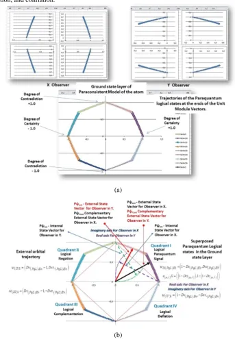
In the first stage of the analysis, we show the trajectory of the logical states in the ground state and its
main equations obtained in Quadrant I of the interlaced PqL bilattice. Moreover, the negation,
complementation, and conflation operations are applied, and the model of the complete atom in the xy plane is formed in the perception of an observer in the vector base X. In the second stage of the analysis, the
modeling equations of the complete atom are presented, and the trajectories of degenerate and nondegenerate
quantum states are highlighted. In the third stage of the analysis, the modeling equations of the energy layers
are derived from the mapping of the degrees of evidence that differs in terms of the direction of rotation,
which is now done clockwise. In this manner, the paraconsistent model of an atom in the xy plane is formed in the perception of an observer in the vector base Y. Finally, the results of an example of the application of
the paraconsistent model of an atom are correlated with the energy values extracted from the Rydberg
formulas and presented based on the hydrogen atom. The results of the hydrogen atom show the curves
obtained from the analysis of signals using only Quadrant I of the interlaced PqL bilattice. With this final
model is presented a method of using Raman spectroscopy signals for the detection of lubricating mineral oil
quality.
2. Materials and Methods
In the construction of the paraconsistent model of the atom, the concepts and equations of PqL and the
logarithmic function of the Shannon entropy H(s) are used. These fundamentals, equations, and concepts are
applied to the in-depth analysis of the interlaced bilattice associated with PqL. In the proposed model, to
represent the probabilistic functions according to the fundamentals of PqL, it is necessary to establish state
vectors with unitary modules and that define the orbital paths and energy layers of the atom.
2.1 State Vectors and Internal and External Orbit Trajectories of Paraquantum Logical States
We present below the representation of the paraquantum logical states related to the unitary module state vectors that are installed in the interlaced bilattice.
2.1.1 Pψint—Internal State Vector
We consider an internal state vector with a unitary module (Pψint) and that has its origin located at the
vertex of the true logical state (t) of the interlaced PqL bilattice. In this point, Dc( ,)= +1 andDct( ,)=0.
Therefore, if the paraquantum logical state of the origin is expressed as =
(
Dc( ,),Dct( ,))
= +( 1, 0), then the variation of the inclination angle of the vector (Pψint) in Quadrant I will be04
in radians. Given that
the modulus is unitary, the variation of the inclination angle
of the vector Pψint will occur in theinterlaced PqL bilattice, with a curvilinear trajectory defined by the paraquantum logical states located at its end.
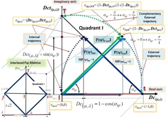
The internal trajectory in Quadrant I of the interlaced PqL bilattice is defined in Eq. (6). 2.1.2 Pψext—External State Vector
For an external state vector with a unitary module (Pψext) and that has its origin at the point equidistant
from the vertices of the interlaced PqL bilattice =
(
Dc( ,),Dct( ,))
=( )0, 0 , the equation of the paraquantum logical states that form the external trajectory in Quadrant I can be described as a function of the value ofand can be expressed as follows:
(
)
( )I= −1 cos( ),sen( )
. (15)
This expression is similar to the following function:
( , )I= −
(
1 Dc( ,),Dct( , ))
, (16)
where and are the degrees of evidence. 2.1.3 PψCext—Complementary External State Vector
The external trajectory of the paraquantum logical states in Quadrant I can be completed for the variation of the inclination angle of another vector, that is, PψCext. With the same values of and, an external
complementary vector (PψCextII) with a unitary module is created simultaneously, with its origin at the point
( ) ( )
(
, , ,)
( )0, 0= Dc Dct =
and its angle of inclination having a variation of
4 2
in radians. With the
same quantitative values of the degrees of evidence, this complementary operation is applied to the degrees of certainty and contradiction, generating the paraquantum logical state( , )=I2(PqL E) 1.
The generated paraquantum logical state establishes the orbital trajectory of the state vector PψI2, whose
inclination presents a variation of 45° to 90°, that is, an angular variation of
4
to radians.
The paraquantum logical state, which features the orbital trajectory at the end of the new complementary state vector, with the completed action in the degrees of certainty and contradiction, is represented by
( ) , II= ( ) , I
in the following expression:
( ), =
(
1− ( ),)
,1− −(
1 ( ),)
II Dct Dc
. (17)
In Quadrant I of the interlaced PqL bilattice, and are represented by probabilistic functions ( )p and
( )p
, which must present results that have their values varying simultaneously in the corresponding intervals,
that is, 0.5( )p 1.0 and , respectively.
Figure 3 shows Quadrant I of the interlaced PqL bilattice with the state vector with a unitary module, which, with the variation of the inclination angle , establishes the internal trajectory of the paraquantum
logical states. In the same mode, the external state vectors PψextI and PψCextI establish the complete external
trajectory of Quadrant I.
Fig. 3. Quadrant I of the interlaced PqL bilattice, with the internal state vector (Pψint) and two external state
vectors (PψextI and PψCextI) that establish the internal and external orbit trajectories of the paraquantum logical
state .
2.2 Representation of the Degrees of Evidence of PqL as Probabilistic Functions
First, we consider that ( )p is a probabilistic function f( )p =X, such that p and it is contained in the closed interval [0,1]. Therefore, p represents a probability value, and the normalized values X and X′ should be adapted to the interlaced PqL bilattice. The two probability values must also be presented to form an annotation. We also consider that as an initial condition, the two probabilistic sources 1 and 2 are out of
2
( ) 0.5p 1.0
phase at the angle Θ, such that in the amplitude variation of the probability value p, the probabilistic function of source 2 generates another function; that is, ( )p =X'. These two probabilistic functions must have the following characteristics: (a) when X is at its maximum unitary value, that is, ( )p =X=1, the difference between X and X′ will be equal to
(
')
( )
Xp = X−X → ( ) 1 1
2
= −
Xp ; (b) when X is at half its maximum value,
that is, ( ) 1 2 = =
p X
, the difference between X and X′ will be null ( ) ' 1 1 0 2 2
= − = − =
Xp X X . From the
reference probability value at source 1, which is considered a degree of favorable evidence( )p , the degree of
unfavorable evidence ( )p under the previously mentioned conditions is derived as follows:
( ) ( ) 2
= p
p
. (18)
From Eq. (4), the degree of certainty of the interlaced PqL bilattice, which is now a probabilistic function,
can be calculated as follows:
( ) ( ) ( )
2
= − p
p p
Dc
. (19)
In the same manner, the degree of contradiction shown in Eq. (5) is also a probabilistic function, which
can be calculated as follows:
. (20)
From Eq. (6), the paraquantum logical state ψPqL that appears in the interlaced PqL bilattice will be
represented by two probabilistic functions, as follows:
( )
p =(
Dc( )
p,Dct( )
p)
. (21) In the representation of the functions, the paraquantum logical state ( )p will form a probabilistictrajectory into the interlaced PqL bilattice. Moreover, the paraquantum logical state ψPqL will form a
probabilistic trajectory out of the interlaced PqL bilattice, with the origin of the state vector at the point equidistant from the vertices, thereby located where Dc( )p =0 and Dct( )p =0. In this case, the paraquantum logical state ψp that forms an external orbit trajectory will be constructed with two probabilistic functions, as
follows:
, (22)
where Dc( )p is obtained using Eq. (19), and Dct( )p is obtained using Eq. (20).
2.3 Representation of Fundamental PqL-Equations
In this work, we will construct a paraconsistent model of the atom using the Shannon entropy to operate
as a probabilistic function representative of the degrees of evidence (μ, λ) in the interlaced PqL bilattice. In this manner, the fundamental PqL-equations as degree of evidence equations will be probabilistic functions
that will be inserted in the energy equations of the paraconsistent model of the atom.
2.3.1 Shannon Normalization Factor
To apply the Shannon entropy function to the PqL equations, we will introduce an adjustment
dimensionless value represented by the symbol l, which will be called the Shannon normalization factor. The lvalue is calculated as follows:
Being that the Shannon entropy from Eq. (12) is represented by the probabilistic logarithmic function
( )s = − [ log + log ]
H k p p q q , the maximum unitary value of H(s) can be obtained when 1 log 2 =
k ; then we will ( ) ( ) ( ) 1
2
= + p −
p p
Dct
( )p = −
(
1 Dc( )p,Dct( )p)
make a representation of k in which the equality of constants is satisfied as
1 log 2
= =l
k . Thus, the
Shannon normalization factor value l is obtained by the equation: 1 log 2 =
l
, where =3.14159265358,
that results atl =1.057402554.
2.3.2 Degrees of Evidence as Shannon Entropy Functions
With these dimensionless values relationships, the function of Shannon entropy for application in PqL, which we namedH( )s PqL, can be represented in a normalized mode as follows:
H( )s PqL= −l[ logp p q+ log ]q , (23) whereis the constant of value ( =3.14159265358...), p is the probability value,
q is the complement of the probability value [q= −(1 p)], and
l is the Shannon normalization factor extracted from k,with 1 1.057402554 log 2
=
l ;
.
The variation of the resulting values of the function H( )s PqLis expressed in the range 0H( )s PqL1; therefore, the Shannon's normalized entropy has the variation values contained within the same range as that
established for the PqL degrees of evidence.
For the paraconsistent model of the atom, the probabilistic function of the degree of favorable evidence of the PqL can be expressed as follows:
(PqL)=H( )s PqL, (24) where H( )s PqL is the Shannon entropy function presented in Eq. (23).
According to Eq. (18), with the inclusion of the Shannon entropy, the probabilistic function of the degree
of unfavorable evidence can be expressed as follows:
, (25)
where H( )s PqL is the probabilistic Shannon entropy function presented in Eq. (23).
With these two last equations, H( )s PqL=1 means high entropy. In this condition, the degree of favorable evidence of the PqL (Eq. 24), will be of unit value (PqL)=1, and the degree of unfavorable evidence (Eq.
25), will be ( ) 2
2 =
PqL
. Likewise, H( )s PqL=0.5 means low entropy. In this condition the degree of favorable evidence, by Eq. (24), will be(PqL)=0.5, and the degree of unfavorable evidence, by Eq. (25), will be
(PqL)=0.5
.
2.4 PqL Energy Equations
The degrees of evidence with their probabilistic representations created by the Shannon entropy function ( )s PqL
H are used in the equations to obtain the degrees of certainty and contradiction resulting in dimensionless
values contained in the range [−1, + 1]. Since the PqL equations are functions that deal with normalized dimensionless values between 0 and 1, when multiplied by a known maximum energy value, they will represent the energy value in each condition expressed by the paraquantum logical states. Thus, in the paraconsistent model of an atom, we can consider that these PqL equations involve quantized energies through the values established by the unit modulus vectors Pψint, Pψext, and PψCextII. In this condition, at the
ground-state level of the atom, the degrees of certainty Dc(PqL)and contradiction Dct(PqL)represent the energy
values, which are obtained using the quantized probabilistic evidence degrees.
From Eq. (19), the probabilistic certainty degree of the ground state (level E1) can be calculated as follows:
( ) 1 ( ) ( )
2
= − s PqL
PqL E s PqL
H
Dc H . (26)
(PqL)
( ) ( )
2
= s PqL
PqL
H
From Eq. (20), the probabilistic contradiction degree of the ground state (level E1) can be calculated as
follows:
(
)
1( )
( )
1 2= + s PqL −
PqL E s PqL
H
Dct H . (27)
The values of the degrees of certainty and contradiction considered in the set of complex numbers £ ,
with their quantized probabilistic functions, represent the energy of the atom. In the proposed paraconsistent
model of an atom, the ground state (level E1) is represented by the point of origin of the real and imaginary
axes, which will be located at the point equidistant from the vertices of the interlaced PqL bilattice. In this representation, the paraconsistent logical state Pql that defines the external orbital trajectory in the ground
state, representing the complex numbers in Quadrant I, is expressed as follows:
I1
(
PqL E)
1= −(
1 Dc(
PqL E)
1,Dct(
PqL E)
1i)
. (28) The probabilistic functions of the paraquantum logical state I PqL E( ) 1 establish the ground state (level E1)and the external orbital trajectory in the ground state of the model of an atom at the end of the state vector
PψI1 with a unitary module; that is, or
( ) ( ) ( ) ( )
2 2
1 1 2 2 1
= − − + + −
s PqL s PqL
E s PqL s PqL
H H
M H H , (29)
where H( )s PqL is the probabilistic Shannon entropy function presented in Eq. (23).
2.5 Analogies between Quantum Mechanics and Paraquantum Logic
With these logical–mathematical considerations, some concepts of PqL can be compared with the
concepts of quantum mechanics on the basis of the equations obtained in Quadrant I of the interlaced PqL bilattice. Therefore, in quantum mechanics, the quantum state is represented by = 0 + 1 and the
vector norm is represented by =2+ 2 . The same paraquantum logical state in quantum
mechanics will be achieved, with the following relations of equality: = −
(
1 Dc(
PqL)
)
and=Dct(
PqL)
. Thequantum state of the quantum mechanics in the PqL is represented by the following well-known Dirac
notation:
. (30)
In general, for n number of states related to En layers of energies:
n = −
(
1 Dc(
PqL)
En)
0 +Dct(
PqL)
En1 . (31)The representation of the degrees of certainty and contradiction and the ground state in level E1 will be
unitary (E1 = 1) and is represented by
( ) ( ) ( ) ( )
2 2
1 1 1
2 2
= − − + + −
s PqL s PqL
Total s PqL s PqL
H H
E H H , (32)
( )
(
)
2(
( ))
21= 1− 1 + 1
E PqL E PqL E
M Dc Dct
(
)
(
1)
0(
)
1= −DcPqL +DctPqL
where the potential energy of the ground state is ( ) ( )
2 1 1
2
= − −
s PqL
P s PqL
H
E H , and the kinetic energy of the
ground state is ( ) ( )
2
1 1
2
= + −
s PqL
c s PqL
H
E H and H( )s PqL is the probabilistic Shannon entropy function
presented in Eq. (23).
2.6 PqL Energy Equations for the Observer in the Vector Base X
In Quadrant I of the interlaced PqL bilattice, the Shannon entropy functions simultaneously create the
trajectories of the paraquantum logical states at the ends of two state vectors, thus establishing the ground
state (level E1) of the quantum state of the particle. The state vector PψCextI constructed with the
complementary action, in relation to the original vector PψextI, has the same characteristics and differs only in
terms of the angular variation. For the X observer, as defined in the mapping shown in Fig. 3, the projections of the real values in the x-axis, which represent the potential energy, and the imaginary values in the y-axis, which represent the kinetic energy, vary proportionally, indicating the equilibrium of values against the
inherent probabilistic uncertainties of quantum mechanics.
2.6.1 Ground State of the Atom in the Paraconsistent Model
The energies of the ground stateare represented by the PqL equations, with the adapted function of the
Shannon entropy having only the probability p as its variable.
Using the logical operations of negation, complementation, and conflation, as well as the fundamentals of
PqL, we will now define the n energy equations that form the n layers of the paraconsistent model of the atom.
Initially, through these operations, the ground-state energy equations of the three other quadrants of the
interlaced PqL bilattice are obtained.
The negation operator applied to the functions of the paraquantum logical states that mark the orbital
trajectory of the particle in the ground stateof Quadrant I produces Quadrant II, as follows:
( )1 ( )1 ( , )
I = II = − → ( )1II =
(
Dc(
PqL En)
−1,Dct(
PqL En)
)
,( )2 ( )2 ( 1, 1)
I = II = − − → ( )2II =
(
Dct,(PqL En) − −1, Dc(PqL En))
.In Quadrant III, the complementation operator applied to the functions of the paraquantum logical states
that mark the orbital trajectory of the particle in the ground state of Quadrant I produces the following
expressions:
( )1 ( )1 ( , )
I = III = − − → (III)1=
(
Dc(
PqL En)
− −1, Dct(
PqL En)
)
,( )2I =(III)2=(−1,1−) → ( )2II =
(
Dct,(
PqL En)
−1,1 (1− −Dc(
PqL En)
))
.In Quadrant IV, the conflation operator applied to the functions of the paraquantum logical states that
mark the orbital trajectory of the particle in the ground state of Quadrant I produces the following
expressions:
( )1= ( )1=( ,− )
‡ I IV → (IV)1= −
(
1 Dc(
PqL En)
,−Dct(
PqL En)
)
,( )2= ( )2=( ,1− )
These PqL logical operations create the paraconsistent model of the atom, where the probabilistic
trajectory of the particle in the ground stateis a unit-radius circle composed of the Shannon entropy functions
introduced in the degrees of certainty and contradiction equations. These probabilistic trajectories related to
the ground stateare shown in the graphics of the results section.
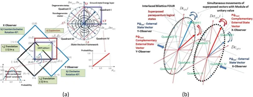
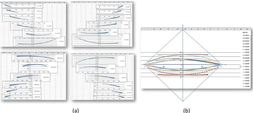
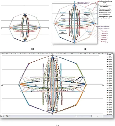
2.7 Energy Layers of Degenerate and Nondegenerate States
In this work, we consider that the layers of the atom that relate to the degenerate states are represented by
the energy that is related to the fundamentally pure state but is not aligned to the x-axis of the real values. In the interlaced PqL bilattice, the degenerate states have different values of contradiction degrees, which bring
them close to the extreme logical state of inconsistency in Quadrants I and II and the extreme logical state of
paracompleteness in Quadrants III and IV.
In the same manner, the layers of the atom that relate to the nondegenerate states are represented by the
energy that is related to the fundamentally pure state. In the interlaced PqL bilattice, the nondegenerate states
are aligned to the x-axis of the real values and thus to the axis of the degrees of certainty. The nondegenerate states have the same values of contradiction degrees and different values of certainty degrees, which bring
them close to the extreme logical state of true (t) in Quadrants I and IV and the extreme logical state of false (f) in Quadrants II and III.
2.7.1 Second Layer of Energy
With these considerations, for the second layer, the degree of favorable evidence μ is expressed in Eq. (24), and that of unfavorable evidence is expressed in Eq. (25).
We can maintain a constant difference between the two degrees of evidence within a reasonable range of
the probability variation p. For this, the degree of unfavorable evidence can be obtained by multiplication with the degree of favorable evidence, such that (PqL EE) 2=(PqL E) 2(PqL E) 2 or
( ) 2 ( ) ( ) 2
= s PqL
PqL EE s PqL
H H
.
(33)
With these values of the degrees of evidence, the degree of certainty for the energy level E2 will have a
constant value over a reasonable range of probability variation p. Therefore,
or
( ) 2 ( ) ( ) ( )
2
= −
s PqL
PqL E s PqL s PqL
H
Dc H H . (34)
Moreover, the degree of contradiction for the energy level E2 can be derived as follows:
( ) 2 ( ) ( ) ( ) 1
2
= + −
s PqL
PqL E s PqL s PqL
H
Dct H H , (35)
where H( )s PqL is the Shannon entropy function presented in Eq. (23).
In the second layer, the degenerate paraquantum logical state will be represented by the function:
(PqL E) 2= −
(
1 Dc(PqL E) 2,Dct(PqL E) 2)
(36)
or by the Dirac notation for the X observer:
, (37)
where Dc(PqL E) 2 is presented in Eq. (34), and Dct(PqL E) 2 is presented in Eq. (35).
(PqL E) 2= (PqL E) 2− (PqL EE) 2
Dc
( )
(
2)
( ) 2(PqL E) 2= −1 DcPqL E 0 +DctPqL E 1
Given the relation to the pure state of the ground state, in the second layer, the pure or nondegenerate
paraquantum logical state will be represented by the complement expressed in Eq. (34) and the function
expressed in Eq. (27), as follows:
(PqL E pure) 2 = −
(
1 Dc(
PqL E)
2,Dct(
PqL E)
1)
. (38)
2.7.2 Third Layer of Energy
In the third layer, the degree of favorable evidence μ is equal to the degree of unfavorable evidence previously presented in Eq. (25). Therefore, or
( ) 3 ( ) 2
= s PqL
PqL E H
. (39)
In this manner, the intermediary degree of unfavorable evidence will be obtained through the square root of (PqL E) 3. Therefore,
( ) 3 ( ) 2
= s PqL
PqL E
H
. (40)
The degree of unfavorable evidence of the third layer will be obtained by multiplication with the degree
of favorable evidence, such that or
( ) 3 ( ) ( )
2 2
= s PqL s PqL
PqL EE
H H
. (41)
With these values of the degrees of evidence, the degree of certainty for the energy level E3 will have a
constant value over a reasonable range of probability variation p. Therefore, the degree of certainty for the
third layer of energy will be computed using or
( ) 3 ( ) ( ) ( )
2 2 2
= −
s PqL s PqL s PqL
PqL E
H H H
Dc . (42)
Moreover, the degree of contradiction for the energy level E3 can be derived as follows:
( ) 3 ( ) ( ) ( ) 1
2 2 2
= + −
s PqL s PqL s PqL PqL E
H H H
Dct . (43)
In the third layer, the degenerate paraquantum logical state will be represented by the function:
(44)
or
( ) 3= −
(
1(
PqL E)
3)
0 +(
PqL E)
31PqL E Dc Dct
, (45)
where Dc(PqL E) 3 is presented in Eq. (42), and Dct(PqL E) 3 is presented in Eq. (43).
In the third layer, the pure or nondegenerate paraquantum logical state will be represented by the
functions expressed in Eqs. (42) and (27), as follows:
(PqL E pure) 3 = −
(
1 Dc(
PqL E)
3,Dct(
PqL E)
1)
.(46)
2.7.3 Fourth Layer of Energy
In the fourth layer, the degree of favorable evidence is equal to the degree of unfavorable evidence previously derived. Therefore, or
( ) 4 ( ) 2
= s PqL
PqL E
H
. (47)
The degree of unfavorable evidence will be obtained through the square root of (PqL E) 4. Therefore, (PqL E) 3= (PqL E) 2
(PqL EE) 3= (PqL E) 3 (PqL E) 3
(PqL E) 3= (PqL E) 3− (PqL EE) 3
Dc
( ) ( )
(
)
(PqL E) 3= −1 DcPqL E3,DctPqL E3
(PqL E) 4= (PqL E) 3
( ) 4 ( ) 2
= s PqL
PqL E
H
.
(48)
The degree of unfavorable evidence of the energy level (E4) of the current state is calculated by
multiplication, such that (PqL EE) 4=(PqL E) 4(PqL E) 4 or
( ) 4 ( ) ( )
2 2
= s PqL s PqL
PqL EE
H H
. (49)
The degree of certainty for energy level E4 can be derived as follows:
( ) 4 ( ) ( ) ( )
2 2 2
= s PqL − s PqL s PqL
PqL E
H H H
Dc . (50)
The degree of contradiction for energy level E4 can be derived as follows:
( ) 4 ( ) ( ) ( ) 1
2 2 2
= s PqL + s PqL s PqL −
PqL E
H H H
Dct . (51)
In the fourth layer, the degenerate paraquantum logical state will be represented by the function:
(52)
or
(
( ))
(
( ))
4 4
1 0 1
= −Dcnd PqL E + Dctnd PqL E
, (53)
where Dc(PqL E) 4 is presented in Eq. (50), and Dct(PqL E) 4 is presented in Eq. (51).
In the fourth layer, the pure or nondegenerate paraquantum logical state will be represented by the
functions expressed in Eqs. (50) and (27), as follows:
(PqL E pure) 3 = −
(
1 Dc(
PqL E)
4,Dct(
PqL E)
1)
.(54)
2.7.4 Fifth Layer of Energy
In the fifth layer, the degree of favorable evidence is equal to the degree of unfavorable evidence previously derived. Therefore, or
( ) 5 ( ) 2
= s PqL
PqL E
H
. (55)
The degree of unfavorable evidence will be obtained through the square root of (PqL E) 5
. Therefore,
( ) 5== ( )2
s PqL PqL E
H
. (56)
Given the relation to the pure state of the fundamental layer, the degree of unfavorable evidence of the energy level (E5) of the current state is calculated by multiplication, such that
or
( ) 5 ( ) ( )
2 2
= s PqL s PqL
PqL EE
H H
. (57)
In this case, the degree of certainty for energy level E5 can be derived as follows:
( ) 5 ( ) ( ) ( )
2 2 2
= −
s PqL s PqL s PqL
PqL E
H H H
Dc . (58)
The degree of contradiction for energy level E5 can be derived as follows:
( ) ( )
(
)
(PqL E) 4= −1 DcPqL E4,DctPqL E4
(PqL E) 5= (PqL E) 4
(PqL EE) 5= (PqL E) 5 (PqL E) 5
( ) 5 ( )2 ( )2 ( )2 1 = + −
s PqL s PqL s PqL
PqL E
H H H
Dct . (59)
In the fifth layer, the degenerate paraquantum logical state will be represented by the function:
(PqL E) 5= −
(
1 Dc(PqL E) 5,Dct(PqL E) 5)
(60)or
=
(
1−Dcnd PqL E( ) 5)
0 +(
Dctnd PqL E( ) 5)
1 , (61) where Dc(PqL E) 5 is presented in Eq. (58), and Dct(PqL E) 5 is presented in Eq. (59).In the fifth layer, the pure or nondegenerate paraquantum logical state will be represented by the functions
expressed Eqs. (58) and (27), as follows:
(
)
(
)
(
)
(PqL E pure) 5 = −1 DcPqL E5,DctPqL E1
.
(62)
2.7.5 Sixth Layer of Energy
In the sixth layer, the degree of favorable evidence is equal to the degree of unfavorable evidence previously derived. Therefore, or
( ) ( ) 6
2
= s PqL
PqL E
H
. (63)
The degree of unfavorable evidence will be obtained through the square root of(PqL E) 6. Therefore,
. (64)
The degree of unfavorable evidence of the energy level (E6) of the current state is calculated by
multiplication, such that (PqL EE) 6=(PqL E) 6(PqL E) 6 or
( ) 6 ( ) ( )
2 2
= s PqL s PqL
PqL EE
H H
. (65)
The degree of certainty for energy level E6 can be derived as follows:
( ) 6 ( )2 ( )2 ( )2
= −
s PqL s PqL s PqL
PqL E
H H H
Dc . (66)
The degree of contradiction for energy level E6 can be derived as follows:
( ) 6 ( )2 ( )2 ( )2 1
= + −
s PqL s PqL s PqL
PqL E
H H H
Dct . (67)
In the sixth layer, the degenerate paraquantum logical state will be represented by the function:
( ) ( )
(
)
(PqL E) 6= −1 DcPqL E6,DcPqL E6
(68)
or
( )
(
1 6)
0(
( ) 6)
1
= − +
DcPqL E DctPqL E
, (69)
where Dc(PqL E) 6 is presented in Eq. (66), and Dct(PqL E) 6 is presented in Eq. (67).
In the sixth layer, the pure or nondegenerate paraquantum logical state will be represented by the
functions expressed in Eqs. (66) and (27), as follows:
(
)
(
)
(
)
(PqL E pure) 6 = −1 DcPqL E6,DctPqL E1
. (70)
(PqL E) 6= (PqL E) 5
( ) ( ) 6
2
= s PqL
PqL E
H
![Figure 1(b) shows the interlaced bilattice of Belnap with the ordering the extreme logical states in their four vertices, t and k and the representations of t, f, ⊺, and ⊥, which denote truth, falsity, both, and none, respectively [22,23][25]](https://thumb-us.123doks.com/thumbv2/123dok_us/8041804.1339031/3.595.125.490.434.591/figure-interlaced-bilattice-ordering-vertices-representations-falsity-respectively.webp)