1
Understanding nuclear binding energy with nucleon mass difference
via strong coupling constant and strong nuclear gravity
U. V. S. Seshavatharam1 & S. Lakshminarayana2
1Honorary Faculty, I-SERVE, Survey no-42, Hitech city, Hyderabad-84, Telangana, India. 2Department of Nuclear Physics, Andhra University, Visakhapatnam-03, AP, India
Emails: [email protected] (and) [email protected] Orcid numbers : 0000-0002-1695-6037 (and) 0000-0002-8923-772X
Abstract: With reference to electromagnetic interaction and Abdus Salam’s strong (nuclear) gravity, 1) Square root of ‘reciprocal’ of the strong coupling constant can be considered as the strength of nuclear elementary charge. 2) ‘Reciprocal’ of the strong coupling constant can be considered as the maximum strength of nuclear binding energy. 3) In deuteron, strength of nuclear binding energy is around unity and there exists no strong interaction in between neutron and proton. 28 3 -1 -2
3.3293665 10 m kg sec s
G being the nuclear gravitational
constant, nuclear charge radius can be shown to be, 2
0 2 s p 1.2392185 fm.
R G m c
2
4.7203105 10 C19s s p
e G m c e being the nuclear elementary charge, proton magnetic moment can be
shown to be, 2 2 1.488055 10 J.T .26 -1
p es mp eG ms p c
2
20.1152072
s c G ms p
being the
strong coupling constant, strong interaction range can be shown to be proportional to exp 1
2
. s Interesting
points to be noted are: An increase in the value of s helps in decreasing the interaction range indicating a more strongly bound nuclear system. A decrease in the value of s helps in increasing the interaction range indicating a more weakly bound nuclear system. One interesting approximation is
10 exp 1
2
.p e s
m m From Z 30
onwards, close to stable mass numbers, nuclear binding energy can be addressed with,
1
1
30
2 19.6 MeV.s s n p
A
B Z m m c Z To improve the accuracy, we tried to understand nuclear binding with two simple terms having a single energy coefficient of 2
2
0
8 10.06 MeV.
s s p
e G m c
With further study, magnitude of the Newtonian gravitational constant can be estimated with nuclear elementary physical constants. One sample relation is,
10 2N s e p s e
G G m m G m c where GN represents the Newtonian gravitational constant. Electroweak gravitational constant can be expressed as, Gew
m me p
10GN.GF being the Fermi’s weak coupling constant, we noticed that, 22G m cs e GF c and
2 2
4 .
F ew
G G c Based on the estimated and recommended values of GF,estimated average value of
11 3 -1 -2 6.674224 10 m kg sec . N
G Finally
it is possible to show that,
30 p e 4 ew
R m m G c and
2
.
s ew e
G G c m
Keywords: strong (nuclear) gravity, nuclear elementary charge, strong coupling constant, nuclear charge radius, beta stability line, nuclear binding energy, nucleon mass difference, Fermi’s weak coupling constant, Newtonian gravitational constant, deuteron, interaction range, super heavy elements.
1. Introduction
Low energy nuclear scientists assume ‘strong interaction’ as a strange nuclear interaction associated with binding of protons and neutrons. High-energy nuclear scientists consider nucleons as composite states of quarks and try to understand the
nature and strength of strong interaction [1] at sub nuclear level. Very unfortunate thing is that, strong interaction is mostly hidden at low energy scales in the form of ‘residual nuclear force’. At this juncture, one important question to be answered and reviewed at the basic level is: How to understand nuclear
2 interactions in terms of sub nuclear interactions?
Unfortunately, the famous nuclear models like, Liquid drop model and Fermi's gas model [2-5] are lagging in answering this question. To find a way, we would like to suggest that, by considering ‘square root’ of reciprocal of the strong coupling constant’
s0.1186 ,
as an index of strength of nuclearelementary charge, nuclear binding energy and nuclear stability can be understood. In this direction, we have developed interesting concepts and produced many semi empirical relations [6-12]. Even though it is in its budding stage, our model seems to be simple and realistic compared to the new integrated model proposed by N. Ghahramany et al [13,14]. It needs further study at a fundamental level.
2. About Strong (nuclear) gravity
Microscopic physics point of view, one very interesting concept is that- elementary particles can be considered as ‘micro black holes’. ‘Strong (nuclear) gravity’ concept proposed by Abdus Salam, C. Sivaram, K.P. Sinha, K. Tennakone, Roberto Onofrio, O. F. Akinto and Farida Tahir [15-20], seems to be very attractive. The main object of unification is to understand the origin of elementary particles mass, (Dirac) magnetic moments and their forces. Right now and till today ‘string theory’ with 10 dimensions is not in a position to explain the unification of gravitational and non-gravitational forces. More clearly speaking it is not in a position to bring down the Planck scale to the nuclear size. The most desirable cases of any unified description are: a) To implement gravity in microscopic physics and
to estimate the magnitude of the Newtonian gravitational constant
GN .b) To develop a model of microscopic quantum gravity.
c) To simplify the complicated issues of known physics.
d) To predict new effects, arising from a combination of the fields inherent in the unified description.
3. About quantum chromo dynamics (QCD)
The modern theory of strong interaction is quantum chromo dynamics (QCD) [21]. It explores baryons and mesons in broad view with 6 quarks and 8
gluons. According to QCD, the four important properties of strong interaction are: 1) color charge; 2) confinement; 3) asymptotic freedom [22]; 4) short-range nature (<10-15 m). Color charge is assumed to be responsible for the strong force to act on quarks via the force carrying agent, gluon. Experimentally it is well established that, strength of strong force depends on the energy through the interaction or the distance between particles. At lower energies or longer distances: a) color charge strength increases; b) strong force becomes ‘stronger’; c) nucleons can be considered as fundamental nuclear particles and quarks seem to be strongly bound within the nucleons leading to ‘Quark confinement’. At high energies or short distances: a) color charge strength decreases; b) strong force gets ‘weaker’; 3) colliding protons generate ‘scattered free quarks leading to ‘Quark Asymptotic freedom’. Based on these points, low energy nuclear scientists assume ‘strong interaction’ as a strange nuclear interaction associated with binding of nucleons. High-energy nuclear scientists consider nucleons as composite states of quarks and try to understand the nature and strength of strong interaction at sub nuclear level.
4. About the semi empirical mass formula
Let A be the total number of nucleons, Z the number of protons and N the number of neutrons. According to the semi-empirical mass formula [2,3,4], nuclear binding energy:
2 2/3
1/3
( 1) ( 2 )
1
p
v s c a
a
Z Z A Z
B a A a A a a
A
A A
Here av15.78 MeV= volume energy coefficient, 18.34 MeV
s
a = surface energy coefficient, 0.71 MeV
c
a = coulomb energy coefficient, 23.21 MeV
a
3
2 2/3
0.4
and 2 2
200
2 c 2 a
A A
Z A Z
A
a a A
By substituting the above value of Z back into
B
one obtains the binding energy as a function of the atomic weight, B A
. Maximizing B A A
/ with respect to A gives the nucleus which is most strongly bound or most stable.5. Three simple assumptions
With reference to our recent paper publications and conference proceedings [6-12], [23-33], we propose the following three assumptions.
1) Nuclear gravitational constant is very large in such a way that,
0 2 2G ms p R
c
(3) 2) Strong coupling constant can be expressed with, 2 2 s s p c G m
(4)
3) There exists a strong elementary charge in such a way that,
2 s p s
s
G m e
e e c (5)
Note: Considering the relativistic mass of proton, it is possible to show that,
4 2 1 1 s p v m c
where
v
can be considered as the speed of proton. Qualitatively, at higher energies, strength of strong interaction seems to decrease with speed of proton. 6. To fix the magnitudes of
Gs, sand es
Considering neutron, proton and electron rest masses, and based on relation (6), proposed nuclear gravitational constant can be estimated. Based on that, other values can be estimated.
28 3 -1 -2
0 2
19
3.3293665 10 m kg sec 2
1.2392185 fm 0.1152072
4.7203105 10 C s s p s s G G m R c e
7. New concepts and semi empirical relations We would like to suggest that,
1) Fine structure ratio can be addressed with,
2 3 2 2 0 7.297352533 10 4 s
s p s p
e c
G m G m
2) Proton magnetic moment can be addressed with
26 -1
1.488055 10 J.T
2 2 s p s p p eG m e m c
3) Neutron magnetic moment can be addressed with
9.816235 10 J.T .27 -12 s n n e e m
4) Nuclear unit radius can be expressed as,
0 2
2G ms p
R c
s
p n
e
e m c m c
5) Root mean square nuclear charge radii [33] can be addressed with,
1 3 , 1 3 1 3 21 0.349 1.262 fm
Z Z A s p N Z R N N G m
Z A Z
c
6) Nuclear potential energy can be understood with ,
2 2 0 20.17225 MeV 4 s s p e G m c
7) Close to stable mass numbers, nuclear binding energy can be understood with a single energy coefficient [30,31] ,
2 3 2
2 2
0 0 0
8 8 8
s p s s
p s p
e G m e e e
m c G m c
10.086124 MeV
8) With reference to
2 , a useful quantum energy constant can be expressed with,
2 3 2 2 0 80.6889925 MeV 4 2 s pe G m E
4 2 1 10.09 MeV 2 2.531 n
where
n = 0,1,2,3,... and
mnm mp e
2.531. 10) Characteristic melting temperature associatedwith proton can be expressed with, 3
12 0.15 10 K 8
proton
B s p c T
k G m
11) Characteristic nuclear neutral mass unit [32] can be addressed with, 546.6365 MeV/ 2
s
c
c
G
.
8. To fit neutron-proton mass difference
Neutron-proton mass difference can be understood with:
2 2 2 3
2
2 2 2 2
0
4
ln ln 6
4
n p s p
e e e
E
m c m c e G m
m c m c m c
9. To fit neutron life time
Neutron life time tn can be understood with the following relation:
2
2 2exp 871.62 sec
n n n p E t m c
m m c
(7)
This can be compared with recommended value [1] of the neutron life time,
880.2 1.0 sec
10. Understanding beta stability line with respect to proton and electron specific charge ratios
Nuclear beta stability line can be addressed with a relation of the form [4],
2 2 2 22 2 4
2 0.0064 2
s
A Z s Z Z s Z
Z
Z Z kZ
(8)
where,
0.00160454 s p e
s
p e
e e
s
m m
G m m c
Based on relation (8), let, 4s k 0.0064182
2 2 2 2 A) 1B) 4
2 9
C 1 1
1 1 D s s s s s s s s A Z
k A N Z
A Z
A Z k
N kZ kA Z kZ A k
11. Nuclear binding energy at stable mass numbers
Interesting points to be noted are:
1. With reference to electromagnetic interaction, and based on proton number,
1s
8.68 can be considered as the maximum strength of nuclear binding energy.2. Z 30 seems to represent a characteristic reference number in understanding nuclear binding of light and heavy atomic nuclides. Based on these points, at stable mass numbers of Z, nuclear binding energy can be expressed by the following simple empirical relation.
2s n p
A
B Z m m c
(10)
1
If Z<30 , coefficient, 1
1
If Z 30 , +1 + 30 15.157
and 15.157 1.29333 MeV 19.6033 MeV
s s Z
Thus, for,
Z 30
19.6033 MeVs
A
B Z
(11)
5 Above and below the stable mass number, binding
energy can be approximately estimated with the following relation.
ln
2s
s s
s
n p
A A
A A A
A
B B m m c
kZ A
(12) It needs further study with reference to unstable nuclides . See table 2 for Z=50.
12. Very simple approach for understanding nuclear stability starting form Z=21 to 118
With this simple method, super heavy elements lower stable mass numbers can be estimated. With even-odd corrections, accuracy can be improved. For
Z 11 ,
1.2 1.2
1.2 1
2.9462 s
s
s
e
A Z Z Z
e
(13)
where,
1 1
6 6
1
1.19732 1.2 s
s
e e
13. Understanding nuclear binding energy of Deuteron
If it is assumed that, there exists no strong interaction in between proton and neutron, nuclear binding of deuteron can be expressed as,
2 2
1
of 2 n p 2.59 MeV
BE H m m c
(14)
2 1
1 1 where,
1
0 0
s
s
s s
e
e e
This can be compared with the experimental value of 2.225 MeV.
14. Understanding nuclear binding energy with two terms (close to stable mass numbers)
Based on the new integrated model proposed by N. Ghahramany et al [13,14],
2 2
2( , ) 3
3
n
N Z N Z m c
B Z N A
Z
(15)
where, Adjusting coefficient
(90 to 100).
if NZ, N Z 0 and if NZ, N Z 1. Readers are encouraged to see references there in [13,14] for derivation part. Point to be noted is that, close to the beta stability line,
2 2
3
N Z
Z
takes care
of the combined effects of coulombic and asymmetric effects. In this context, we would like suggest that,
2 2
2
2 0
Constant 90 to 100
10.09MeV 8
n n
s
s p
m c m c
e G m c
(16)
Proceeding further, with reference to relation (8), it is also possible to show that, for Z
40 to 83 ,
close to the beta stability line,2 2
s
s
N Z
kA Z Z
(17)
2 2
3 3
s s
N Z kA Z
Z
(18)
Based on the above relations and close to the stable mass numbers of
Z 5 to 118 ,
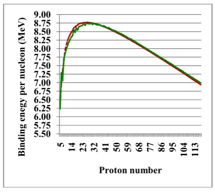
with a common energy coefficient of 10.06 MeV, we would like to suggest two terms for fitting and understanding nuclear binding energy.First term helps in increasing the binding energy and can be considered as,
Term_1As10.06 MeV (19) Second term helps in decreasing the binding energy and can be considered as,
Term_2 3.531 10.06 MeV
2.531 s
kA Z
6 where
22
1
ln 2.531.
1 3.531 1 2.531 1 ln
n p
e
m m c
m c k
k
Thus, binding energy can be fitted with,
3.531 10.06 MeV 2.531
s
s
A s
kA Z
B A
(21)
See the following figure 1. Dotted red curve plotted with relations (8) and (21) can be compared with the green curve plotted with the standard semi empirical mass formula (SEMF).
Figure 1: Binding energy per nucleon close to stable mass numbers of Z = 5 to 118
15. To fix the magnitude of Fermi’s weak coupling constant
With trial-error we noticed that,
0 2
2 2
2
s p p F
e
s e F
G m m G
R
c m c
G m G
c c (22)
where GF is the Fermi’s weak coupling constant [1,19] and GF Characteristic electroweak length.
c
Based on this relation,
3 2 4 4 e s F p m G m c
(23)
3 2 2 2
4 3 2 62 3 2 4 4 1 2
1.4400414 10 J.m
e s e
F
s p
s e
m G m
G
m c c
G m c c (24)
Recommended value of 62 3
1.43586 10 J.m . F
G It
may be noted that, relations (23) and (24) seem to play a key role in understanding the basics of final unification and needs further study.
16. To fix the magnitude of Newtonian Gravitational constant
With reference to Planck scale and considering the following semi empirical relation, magnitude of the Newtonian gravitational constant
GN can be fitted [23, 34].1 1
2 12 12
p s p s s s
e N N
m G m G e G
m c G eG
(25)
Based on relations (22) to (25),
12 12 3 2 4 4 p p s e s
N e p W e
m m
G m
G m m cF m
(26)
10 10 2 5 2 1 2
N e F
e
s p
e s e
N s
p
p N
s
e e
G m G
c m c
G m
m G m
G G
m c
m G c
G m m
(27)
where Compton wavelength of electron. e
m c
Based
on the recommended and estimated values of GF,
11 3 -1 -2
62 3 6.66937197 10 m kg sec where 1.43586 10 J.m
N F G G
11 3 -1 -2
62 3 6.679076 10 m kg sec where 1.440414 10 J.m
N F G G
5.50 5.75 6.00 6.25 6.50 6.75 7.00 7.25 7.50 7.75 8.00 8.25 8.50 8.75 9.00
5 14 23 32 41 50 59 68 77 86 95
7
Average value of 11 3 -1 -2
6.674224 10 m kg sec . N
G
In terms of nuclear charge radius, 11 5 2 0 3 1 4 e F N p
m c G R
G
m
(28)
Accuracy of
GN seems to depend on
G Rs, , ,0 s GF
.17. To fix the magnitude of electroweak gravitational constant
According to Roberto Onofrio [19], electro weak scale gravitational constant is roughly 1033 times the Newtonian gravitational constant. In this context, we would like suggest that,
10 p ew N e m G G m
(29)
where 2.90723 10 m kg sec22 3 -1 -2 ew
G can be
considered as the electroweak gravitational constant. Based on this idea,
11
0 3 3
4 4
p ew p N
e e
m G m G
R
m c m c
(30)
where 4G3ew
c
can be called as the electroweak
Planck length.
2
3 2
4 ew 4 ew F G G G c c c
(31)
Based on relation (27),
52 2
p N
s ew
e e e
m G c c
G G
m m m
(32)
Characteristic electroweak mass and its Schwarzschild radius can be expressed as,
2 584.983 GeV/ ew ew c M c G
(33)
19
2 3
2 4
6.74642 10 m
ew ew ew
G M G
c c
(34)
2 ew
p ew p s p e
M c c
m G m G m m
(35)
ew s
e ew
M G
m G
(36)
18. To understand the range of strong interaction
One strange approximation is, 10
2
32 32
1 exp
4.356 10 5.259 10 p e s m m (37)
Based on above relations, strong interaction range can be understood with the following relation.
0 2 3
4 1
exp p N
s e F
m G c
R
m c G
(38)
It seems interesting to infer that,
a) 12 s
and 2
1 exp s
play a crucial role in
deciding the strong interaction range.
b) An increase in the value of s helps in decreasing the interaction range. This may be an indication of more strongly bound nuclear system.
c) A decrease in the value of s helps in increasing the interaction range. This may be an indication of more weakly bound nuclear system.
8 Even though our approach to nuclear physics seems
to be speculative, proposed assumptions show a wide range of applications embedded with in-depth physical meaning connected with low energy nuclear physics and high energy nuclear physics. With reference to the famous semi empirical mass formula having 5 different energy terms and 5 different energy coefficients, qualitatively and quantitatively, our proposed relations (8), (10) and (21) are very simple to follow and a special study seems to be required for understanding the binding energy of isotopes above and below the stability line. We are working in this direction.
With further research, current nuclear models and strong interaction concepts can be studied in a unified manner with respect to strong nuclear gravity. Finally, value of the Newtonian gravitational constant can be estimated with nuclear elementary physical constants.
Acknowledgements
Author Seshavatharam is indebted to professors shri M. NagaphaniSarma, Chairman, shri K.V. Krishna Murthy, founder Chairman, Institute of Scientific Research in Vedas (I-SERVE), Hyderabad, India and Shri K.V.R.S. Murthy, former scientist IICT (CSIR), Govt. of India, Director, Research and Development, I-SERVE, for their valuable guidance and great support in developing this subject.
References
[1] C. Patrignani et al. (Particle Data Group), Chin. Phys. C, 40, 100001 (2016) and 2017 update [2] Weizsäcker, Carl Friedrich von, On the theory of
nuclear masses; Journal of Physics 96 pages 431- 458 (1935)
[3] W. D. Myers et al. Table of Nuclear Masses according to the 1994 Thomas-Fermi Model.(from nsdssd.lbl.gov)
[4] P. Roy Chowdhury et al. Modified Bethe-Weizsacker mass formula with isotonic shift and new driplines. Mod.Phys.Lett. A20 1605-1618. (2005)
[5] J.A. Maruhn et al., Simple Models of Many-Fermion Systems, Springer-Verlag Berlin Heidelberg 2010. Chapter 2, page:45-70. [6] Seshavatharam U. V. S, Lakshminarayana, S.,
A new approach to understand nuclear stability and binding energy. Proceedings of the DAE-BRNS Symp. onNucl. Phys. 62, 106-107 (2017) [7] Seshavatharam U. V. S, Lakshminarayana, S.,
On the Ratio of Nuclear Binding Energy &
Protons Kinetic Energy. Prespacetime Journal, Volume 6, Issue 3, pp. 247-255 (2015)
[8] Seshavatharam U. V. S, Lakshminarayana, S., Consideration on Nuclear Binding Energy Formula. Prespacetime Journal, Volume 6, Issue 1, pp.58-75 (2015)
[9] Seshavatharam U. V. S, Lakshminarayana, S., Simplified Form of the Semi-empirical Mass Formula. Prespacetime Journal, Volume 8, Issue 7, pp.881-810 (2017)
[10]Seshavatharam U. V. S, Lakshminarayana, S., On the role of strong coupling constant and nucleons in understanding nuclear stability and binding energy. Journal of Nuclear Sciences, Vol. 4, No.1, 7-18, (2017)
[11]Seshavatharam U. V. S, Lakshminarayana, S., A Review on Nuclear Binding Energy Connected with Strong Interaction. Prespacetime Journal, Volume 8, Issue 10, pp. 1255-1271 (2018)
[12]U. V. S. Seshavatharam, Lakshminarayana S. To unite nuclear and sub-nuclear strong interactions. International Journal of Physical Research, 5 (2) 104-108 (2017)
[13]Ghahramany et al. New approach to nuclear binding energy in integrated nuclear model. Journal of Theoretical and Applied Physics 2012, 6:3
[14]N. Ghahramany et al. Stability and Mass Parabola in Integrated Nuclear Model. Universal Journal of Physics and Application 1(1): 18-25, (2013).
[15]K. Tennakone. Electron, muon, proton, and strong gravity. Phys. Rev. D 10, 1722 (1974). [16] Sivaram, C, Sinha, K. Strong gravity, black holes,
and hadrons. Physical Review D. 16 (6): 1975-1978. (1977).
[17] Salam, Abdus; Sivaram, C. Strong Gravity Approach to QCD and Confinement. Modern Physics Letters A, 8 (4): 321–326. (1993). [18]C. Sivaram et al. Gravity of Accelerations on
Quantum Scales. Preprint, arXiv:1402.5071 [19]Roberto Onofrio. On weak interactions as
short-distance manifestations of gravity. Modern Physics Letters A 28, 1350022 (2013)
[20]O. F. Akinto, Farida Tahir. Strong Gravity Approach to QCD and General Relativity. arXiv:1606.06963v3 (2017)
9 [22]David J. Gross. Twenty Five Years of symptotic
Freedom. Nucl.Phys.Proc.Suppl. 74, 426-446 (1999)
[23]Seshavatharam U.V.S & Lakshminarayana S, A Virtual Model of Microscopic Quantum Gravity. Prespacetime Journal, Vol 9, Issue 1, pp. 58-82 (2018).
[24]Seshavatharam U.V.S & Lakshminarayana S, To confirm the existence of nuclear gravitational constant, Open Science Journal of Modern Physics. 2(5): 89-102 (2015).
[25]Seshavatharam U.V.S & Lakshminarayana S, Towards a workable model of final unification. International Journal of Mathematics and Physics 7, No1,117-130. (2016)
[26]U. V. S. Seshavatharam and S. Lakshminarayana. Understanding the basics of final unification with three gravitational constants associated with nuclear, electromagnetic and gravitational interactions. Journal of Nuclear Physics, Material Sciences, Radiation and Applications Vol-4, No-1, 1-19. (2017)
[27]U. V. S. Seshavatharam et al. Understanding the constructional features of materialistic atoms in the light of strong nuclear gravitational coupling. Materials Today: 3/10PB, Proceedings 3 pp. 3976-3981 (2016)
[28]U. V. S. Seshavatharam, Lakshminarayana S. Lakshminarayana. To Validate the Role of
Electromagnetic and Strong Gravitational Constants via the Strong Elementary Charge. Universal Journal of Physics and Application 9(5): 210-219 (2015)
[29] On the role of ‘reciprocal’ of the strong coupling constant in nuclear structure. Journal of Nuclear Sciences, Vol. 4, No.2, 31-44. (2017)
[30]Fermi scale applications of strong (nuclear) gravity-1 Proceedings of the DAE Symp. on Nucl. Phys. 63 72-73. (2108)
[31] Seshavatharam, U.V.S., & Lakshminarayana S., On the Possible Existence of Strong Elementary Charge & Its Applications. Prespacetime Journal, Volume 9, Issue 7, pp. 642-651 (2018)
[32] Seshavatharam U.V.S & Lakshminarayana S. Scale Independent Workable Model of Final Unification. Universal Journal of Physics and Application 10(6): 198-206. (2016)
[33]T. Bayram, S. Akkoyun, S. O. Kara and A. Sinan, New Parameters for Nuclear Charge Radius Formulas, Acta Physica Polonica B. 44( 8), 1791-1799. (2013).
[34]Seshavatharam, U.V.S., & Lakshminarayana S., Analytical estimation of the gravitational constant with atomic and nuclear physical constants. Proceedings of the DAE-BRNS Symp. on Nucl. Phys. 60, 850-851 (2015)
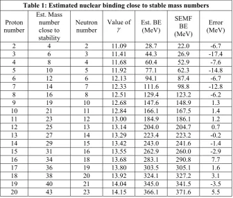
Table 1: Estimated nuclear binding close to stable mass numbers
Proton number
Est. Mass number close to stability
Neutron number
Value of
Est. BE (MeV)
SEMF BE (MeV)
Error (MeV)
2 4 2 11.09 28.7 22.0 -6.7
3 6 3 11.41 44.3 26.9 -17.4
4 8 4 11.68 60.4 52.9 -7.6
5 10 5 11.92 77.1 62.3 -14.8
6 12 6 12.13 94.1 87.4 -6.7
7 14 7 12.33 111.6 98.8 -12.8
8 16 8 12.51 129.4 123.2 -6.2
9 19 10 12.68 147.6 148.9 1.3
10 21 11 12.84 166.1 167.5 1.4
11 23 12 13.00 184.9 186.1 1.2
12 25 13 13.14 204.0 204.7 0.7
13 27 14 13.29 223.4 223.2 -0.2
14 29 15 13.42 243.0 241.6 -1.4
15 31 16 13.55 262.9 260.0 -2.9
16 34 18 13.68 283.1 290.8 7.7
17 36 19 13.80 303.5 305.1 1.6
18 38 20 13.92 324.1 327.2 3.1
19 40 21 14.04 345.0 341.5 -3.5
10
21 45 24 14.26 387.4 389.6 2.2
22 47 25 14.37 408.9 407.5 -1.4
23 49 26 14.48 430.6 425.2 -5.4
24 52 28 14.58 452.5 454.6 2.0
25 54 29 14.68 474.7 468.9 -5.8
26 56 30 14.78 497.0 489.6 -7.4
27 59 32 14.88 519.5 515.2 -4.3
28 61 33 14.97 542.2 532.5 -9.7
29 63 34 15.07 565.0 549.7 -15.4
30 66 36 15.16 588.1 577.9 -10.2
31 68 37 15.16 607.7 592.0 -15.7
32 71 39 15.16 627.3 619.8 -7.5
33 73 40 15.16 646.9 636.6 -10.3
34 75 41 15.16 666.5 653.3 -13.2
35 78 43 15.16 686.1 677.9 -8.2
36 80 44 15.16 705.7 697.0 -8.7
37 83 46 15.16 725.3 721.3 -4.0
38 85 47 15.16 744.9 737.6 -7.3
39 88 49 15.16 764.5 761.6 -2.9
40 90 50 15.16 784.1 780.2 -3.9
41 93 52 15.16 803.7 803.9 0.2
42 95 53 15.16 823.3 819.7 -3.6
43 98 55 15.16 842.9 843.2 0.2
44 100 56 15.16 862.5 861.2 -1.3
45 103 58 15.16 882.1 884.4 2.2
46 106 60 15.16 901.7 909.6 7.9
47 108 61 15.16 921.3 922.7 1.4
48 111 63 15.16 940.9 947.6 6.7
49 113 64 15.16 960.5 962.8 2.3
50 116 66 15.16 980.2 987.5 7.3
51 119 68 15.16 999.8 1009.7 9.9
52 121 69 15.16 1019.4 1024.6 5.2
53 124 71 15.16 1039.0 1046.5 7.6
54 127 73 15.16 1058.6 1070.4 11.9
55 129 74 15.16 1078.2 1085.1 6.9
56 132 76 15.16 1097.8 1108.7 11.0
57 135 78 15.16 1117.4 1130.1 12.7
58 138 80 15.16 1137.0 1153.3 16.3
59 140 81 15.16 1156.6 1165.6 9.0
60 143 83 15.16 1176.2 1188.5 12.3
61 146 85 15.16 1195.8 1209.3 13.5
62 149 87 15.16 1215.4 1231.9 16.5
63 151 88 15.16 1235.0 1245.9 10.9
64 154 90 15.16 1254.6 1268.2 13.6
65 157 92 15.16 1274.2 1288.4 14.2
66 160 94 15.16 1293.8 1310.4 16.6
67 163 96 15.16 1313.4 1330.4 17.0
68 166 98 15.16 1333.0 1352.0 19.0
69 169 100 15.16 1352.6 1371.7 19.1
70 171 101 15.16 1372.2 1385.1 12.9
71 174 103 15.16 1391.8 1404.5 12.7
72 177 105 15.16 1411.4 1425.7 14.2
73 180 107 15.16 1431.0 1444.8 13.8
11
75 186 111 15.16 1470.2 1484.6 14.3
76 189 113 15.16 1489.8 1505.1 15.3
77 192 115 15.16 1509.4 1523.7 14.3
78 195 117 15.16 1529.0 1544.0 14.9
79 198 119 15.16 1548.6 1562.4 13.7
80 201 121 15.16 1568.2 1582.3 14.1
81 204 123 15.16 1587.8 1600.5 12.6
82 207 125 15.16 1607.4 1620.2 12.7
83 210 127 15.16 1627.0 1638.1 11.0
84 213 129 15.16 1646.7 1657.5 10.8
85 216 131 15.16 1666.3 1675.2 8.9
86 219 133 15.16 1685.9 1694.3 8.5
87 223 136 15.16 1705.5 1718.6 13.1
88 226 138 15.16 1725.1 1737.5 12.4
89 229 140 15.16 1744.7 1754.6 10.0
90 232 142 15.16 1764.3 1773.2 9.0
91 235 144 15.16 1783.9 1790.2 6.3
92 238 146 15.16 1803.5 1808.5 5.1
93 241 148 15.16 1823.1 1830.2 7.1
94 245 151 15.16 1842.7 1848.3 5.6
95 248 153 15.16 1862.3 1864.8 2.5
96 251 155 15.16 1881.9 1882.6 0.7
97 254 157 15.16 1901.5 1898.9 -2.6
98 258 160 15.16 1921.1 1922.7 1.6
99 261 162 15.16 1940.7 1938.7 -2.0
100 264 164 15.16 1960.3 1956.1 -4.2
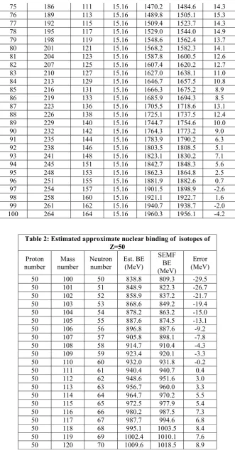
Table 2: Estimated approximate nuclear binding of isotopes of Z=50
Proton
number number Mass Neutron number Est. BE (MeV)
SEMF BE (MeV)
Error (MeV)
50 100 50 838.8 809.3 -29.5
50 101 51 848.9 822.3 -26.7
50 102 52 858.9 837.2 -21.7
50 103 53 868.6 849.2 -19.4
50 104 54 878.2 863.2 -15.0
50 105 55 887.6 874.5 -13.1
50 106 56 896.8 887.6 -9.2
50 107 57 905.8 898.1 -7.8
50 108 58 914.7 910.4 -4.3
50 109 59 923.4 920.1 -3.3
50 110 60 932.0 931.8 -0.2
50 111 61 940.4 940.7 0.4
50 112 62 948.6 951.6 3.0
50 113 63 956.7 960.0 3.3
50 114 64 964.7 970.2 5.5
50 115 65 972.5 977.9 5.4
50 116 66 980.2 987.5 7.3
50 117 67 987.7 994.6 6.8
50 118 68 995.1 1003.5 8.4
50 119 69 1002.4 1010.1 7.6
12
50 121 71 1016.7 1024.4 7.8
50 122 72 1023.6 1032.3 8.7
50 123 73 1030.5 1037.7 7.3
50 124 74 1037.2 1045.1 7.9
50 125 75 1043.8 1050.1 6.3
50 126 76 1050.3 1056.9 6.6
50 127 77 1056.7 1061.4 4.7
50 128 78 1063.0 1067.8 4.8
50 129 79 1069.2 1071.8 2.6
50 130 80 1075.3 1077.7 2.4
50 131 81 1081.3 1081.4 0.0
50 132 82 1087.3 1086.9 -0.4
50 133 83 1093.1 1090.1 -3.1
50 134 84 1098.9 1095.1 -3.7
50 135 85 1104.5 1098.0 -6.6
50 136 86 1110.1 1102.7 -7.5
50 137 87 1115.6 1105.1 -10.5
50 138 88 1121.0 1109.4 -11.6
50 139 89 1126.4 1111.5 -14.9