Principal Longevity, Leadership Behaviors, and Student Academic Achievement

University of South Carolina

Scholar Commons

Theses and Dissertations

1-1-2013

Geomorphic Variation of A Transitional River: Blue

Ridge to Piedmont, South Carolina

Tanner Arrington

University of South Carolina

Follow this and additional works at:https://scholarcommons.sc.edu/etd Part of theGeography Commons

This Open Access Thesis is brought to you by Scholar Commons. It has been accepted for inclusion in Theses and Dissertations by an authorized administrator of Scholar Commons. For more information, please contactdillarda@mailbox.sc.edu.

Recommended Citation

G

V

T

R

:

B

R

P

,

S

C

by

Tanner Arrington Bachelor of Arts

The University of Texas at Austin, 2010

Submitted in Partial Fulfillment of the Requirements For the Degree of Master of Science in

Geography

College of Arts and Sciences University of South Carolina

2013 Accepted by:

Allan James, Director of Thesis John Kupfer, Reader

Ray Torres, Reader

ii

iii

DEDICATION

iv

ACKNOWLEDGMENTS

I’d like to thank Dr. Allan James for advising me through the progress of this

research

.

v

ABSTRACT

Field data was collected systematically to characterize the geomorphic variations in a river transition from the southern Blue Ridge to the Piedmont physiographic regions in South Carolina. Ten study reaches were surveyed for cross-sections and longitudinal profiles. Surface grid samples of bed material collected. Downstream hydraulic

geometry and downstream fining of bed material were analyzed using traditional power functions and exponential decay relationships. Reach-scale channel bed morphology (bedforms) was analyzed under the assumption that the transition in bedforms is related to changes in hydraulic geometry and sediment characteristics. Well-developed downstream trends of hydraulic geometry variables (width, depth and velocity) and bed material fining were observed. However, variations within the general trends reflect the

vi

vii

PREFACE

The idea for this research was developed after noticing the apparently high level of interest in local rivers from land owners and citizens around the Middle Saluda River. Many fences and lawns display the yard-signs of local river interest organizations. Two recent river “restoration” projects have been completed in the area, on the Middle Saluda River in 2009 and the South Saluda River in 2011. Further, debates broke out between different groups over the restoration approach on the South Saluda, resulting in a lawsuit that attempted to halt the project. Debate about river restoration has been ongoing for well over a decade (see Bernhardt et al. 2007), with projects achieving varying degrees of “success”. While states like Maryland and North Carolina have completed large numbers of restoration projects, South Carolina joined river restoration

viii

TABLE OF CONTENTS

DEDICATION ... iii

ACKNOWLEDGMENTS ... iv

ABSTRACT ...v

PREFACE ... vii

LIST OF TABLES ...x

LIST OF FIGURES ... xi

CHAPTER 1INTRODUCTION AND CONCEPTUAL FRAMEWORK ... 1

1.1INTRODUCTION ... 1

1.2CONCEPTUAL FRAMEWORK ... 2

CHAPTER 2SUBMITTED MANUSCRIPT ... 8

2.1ABSTRACT ... 10

2.2INTRODUCTION ... 11

2.3PHYSICAL SETTING ... 17

ix

2.5RESULTS ... 24

2.6DISCUSSION AND CONCLUSION ... 35

2.7REFERENCES ... 39

CHAPTER 3EXTENDED METHODOLOGY RESULTS AND DISCUSSION ... 40

3.1EXTENDED METHODS ... 40

3.2EXTENDED RESULTS ... 49

3.3EXTENDED DISCUSSION ... 54

CONCLUSION ... 57

REFERENCES ... 58

APPENDIX A–TABLES OF DATA ... 63

x

LIST OF TABLES

TABLE 2.1EXPLANATION OF VARIABLES AND CALCULATIONS ... 23

TABLE 2.2SUMMARY OF DATA AND CALCULATIONS ... 24

TABLE 3.1 DOWNSTREAM TRENDS IN GRAPHIC ARITHMETIC STATISTICS ... 52

TABLE A.1BASIN DATA ... 63

TABLE A.2HYDRAULICS DATA ... 64

TABLE A.3BED MATERIAL PARTICLE B-AXIS DIMENSIONS (MM) ... 65

TABLE A.4GRAPHIC ARITHMETIC BED MATERIAL STATISTICS... 66

TABLE A.5INDICES AND RATIOS DATA ... 67

xi

LIST OF FIGURES

FIGURE 2.1CONCEPTUAL BEDFORM TYPES ... 16

FIGURE 2.2STUDY WATERSHED LOCATION AND TOPOGRAPHY ... 19

FIGURE 2.3DOWNSTREAM HYDRAULIC GEOMETRY RELATIONSHIPS ... 25

FIGURE 2.4DOWNSTREAM FINING OF D84 ... 27

FIGURE 2.5REGIME DIAGRAM ... 31

FIGURE 2.6PLOTS OF BEDFORM ROUGHNESS ... 33

FIGURE 2.7SLOPE-AREA PLOT FOR MIDDLE SALUDA RIVER ... 35

FIGURE 3.1LONGITUDINAL PROFILE OF BANKFULL INDICATORS –SITE 2 ... 42

FIGURE 3.2LONGITUDINAL PROFILE OF THE CHANNEL BED –SITE 2 ... 42

FIGURE 3.3LONGITUDINAL PROFILE OF BANKFULL INDICATORS –SITE 7 ... 44

FIGURE 3.4LONGITUDINAL PROFILE OF THE CHANNEL BED –SITE 7 ... 44

FIGURE 3.5CROSS-SECTION AND BANKFULL ESTIMATION AT SITE 3 ... 46

FIGURE 3.6HIGHLY ERODIBLE GRUS IN GAP CREEK ... 48

xii

FIGURE 3.8TRENDS IN GRAPHIC ARITHMETIC STATISTICS WITH GRADIENT ... 54

FIGURE 3.9CONCEPTUAL LONGITUDINAL PROFILE OF INFILLED MORPHOLOGY AT SITE 8 ... 55

FIGURE B.1CROSS-SECTION AND LONGITUDINAL BANKFULL PROFILE,SITE 1 ... 68

FIGURE B.2CROSS-SECTION AND LONGITUDINAL BANKFULL PROFILE,SITE 2 ... 69

FIGURE B.3CROSS-SECTION AND LONGITUDINAL BANKFULL PROFILE,SITE 3 ... 69

FIGURE B.4CROSS-SECTION AND LONGITUDINAL BANKFULL PROFILE,SITE 4 ... 70

FIGURE B.5CROSS-SECTION AND LONGITUDINAL BANKFULL PROFILE,SITE 5 ... 70

FIGURE B.6CROSS-SECTION AND LONGITUDINAL BANKFULL PROFILE,SITE 6 ... 71

FIGURE B.7CROSS-SECTION AND LONGITUDINAL BANKFULL PROFILE,SITE 7 ... 71

FIGURE B.8CROSS-SECTION AND LONGITUDINAL BANKFULL PROFILE,SITE 8 ... 72

FIGURE B.9CROSS-SECTION AND LONGITUDINAL BANKFULL PROFILE,SITE 9 ... 72

1

CHAPTER 1

INTRODUCTION AND CONCEPTUAL FRAMEWORK

1.1 I

The Middle Saluda River emerges from the Blue Ridge Escarpment in northern South Carolina and flows through a transition zone from the Blue Ridge to the Piedmont physiographic regions. The goal of this research is to explore downstream hydraulic geometry (DHG), bed sediment and reach-scale channel bedforms through the course of this transition zone. Many well-established concepts in fluvial geomorphology were developed with low gradient rivers. The applicability of such concepts to steeper gradient rivers has been increasingly addressed in the literature (e.g. Wohl, 2004) and transitions in fluvial systems have been described as zones of variability in fluvial processes (Montgomery and Buffington, 1997; Wohl and Merritt, 2008; Fryirs and Brierley, 2010). However, mountain and transitional rivers remain less understood than lower gradient rivers (Wohl and Merritt, 2008). Further, research in fluvial

2

unique transition in the fluvial system with implications for river restoration and management.

The goal of this thesis is to study changes in fluvial geomorphology through a transition from the Blue Ridge to the Piedmont physiographic regions in South Carolina. This thesis utilizes the “manuscript style” of documentation, where an article (Arrington and James, in review) submitted to Physical Geography, a peer-reviewed journal, is used as a chapter in the thesis. As such, the thesis is organized so that the submitted article (hereafter referred to as the ‘manuscript’), Chapter 2, is the main body of the thesis. Chapter 1 is an extended literature review that includes additional discussions that were not included in the submitted manuscript. Chapter 3 expounds upon the research process and discusses implications that are not covered in the manuscript. The Appendices include detailed tables of data and figures. Due to the nature of the manuscript style, some information may be redundant through different sections.

1.2

C

F

This research examines downstream trends in three sets of fluvial features through the transition from the Blue Ridge to the Piedmont:

(1) Channel form and downstream hydraulic geometry (DHG) (2) Bed material size

3

Literature on mountain rivers from the first two components is considered first. The third component is related to the first two based on the assumption that channel morphology (bedforms) is a function of the transport capacity of the river and sediment supply (Montgomery and Buffington, 1997). Thus, the third component draws on literature from the first two. However, research has developed specific to the hydraulic and sediment conditions associated with different bedform types. This literature will be discussed lastly in this chapter. Each of these topics is reviewed in the manuscript (Chapter 2) and those discussions are not repeated here in their entirety. This

discussion is intended to augment discussions of the three features with greater detail than is presented in the manuscript.

1.2.1 DOWNSTREAM HYDRAULIC GEOMETRY

Conceptual theory of downstream variations in channel width ( ), mean flow depth ( ) and velocity ( ) suggests that systematic changes in channel dimensions can be

expressed as relatively simple power relationships with discharge known as downstream hydraulic geometry (DHG) (Leopold and Maddock, 1953). Their form typically follows:

(Eq. 1)

(Eq. 2)

, (Eq. 3)

4

These relationships assume that alluvial channels adjust to changes in discharge or sediment supply toward an approximate equilibrium state (Wohl et al., 2004; Faustini et al., 2009). This general relationship has held up well in regional-scale studies in the United States and is widely used. For instance, Faustini et al. (2009) developed regional DHG curves for wadeable streams across the conterminous United States.

For alluvial rivers, DHG assumes that a deformable boundary is adjusted to the sufficient power of the regular magnitude and duration of flows in the basin (Leopold and Maddock, 1953). The range of flows that are effective in forming the channel are moderate in magnitude and frequency (Wolman and Miller, 1960), and are often

described by a relatively frequently occurring discharge; i.e., the bankfull discharge. The use of DHG for mountain rivers has produced mixed results (Wohl, 2004) suggesting that some mountain rivers have other variables that prevent channel geometry from

adjusting to bankfull flows. These differences may include spatially and temporally stochastic inputs of coarse sediment, differences in tectonic uplift across the basin, differences in resistance among bed material lithologies, large woody debris loadings, and small discharge magnitudes of frequently occurring events (Wohl, 2004). This is corroborated by results of highly variable stream power in mountain basins (Fonstad, 2003; Wohl et al., 2004). Wohl (2004) defined steep channels as those with an average gradient of at least 0.002 m/m and compared mountain drainages with well-developed and poorly developed DHG. She identified a threshold of the ratio of cross-sectional stream power to the 84th percentile of bed material (Ω/D84) of 10,000 kg/s3 that can be

5

channel reach with coarse bed material, lack of sufficient discharge, lack of slope, or a combination of these may not display DHG trends (i.e. boundary is not adjustable under ‘bankfull discharge’ conditions). As these factors change, however, a critical condition is ultimately reached beyond which the alluvial boundaries are frequently subjected to morphogenesis, which creates channel forms that change systematically downstream with discharge. The suggestion of this threshold as a limit to well-developed DHG has not been explored further in the literature.

1.2.2 DOWNSTREAM FINING

Downstream fining is the observation that bed material size decreases with distance downstream and is related to hydraulic variables, particularly slope (Knighton 1998). Varying explanations have been given for downstream fining, including abrasion of bed materials (e.g. Kodama, 1994a; 1994b), hydraulic sorting, and transport of bed material (e.g. Wilcock and McArdell, 1993; Ferguson et al., 1996; Gomez et al., 2001). However, applicability of the concept of downstream fining is scale dependent and variable depending on local conditions. Tributary and local sediment inputs are important to downstream textural variations in bed material (Best, 1988; Rice, 1998; Rădoane et al., 2008). Rădoane et al. (2008) have an especially robust dataset of field samples in Romania that demonstrate the influence of tributary inputs on particle size distributions of the channel bed. They find that tributary inputs create abrupt

6

knick points while tributaries have little effect (Ferguson and Ashworth, 1991; Surian, 2002). However, certain homogeneous conditions within a basin may develop a continuous fining trend with few disruptions and a rapid gravel to sand transition

(Gomez et al., 2001). Sambrook Smith and Ferguson (1995) describe the abrupt gravel to sand transition as a “threshold” between two different types of rivers rather than a continuation of the downstream fining process. Other studies suggest that due to bimodal sediment distributions and selective transport, the gravel to sand transition is more gradual than has often been assumed (Pitlick et al., 2008; Singer, 2008).

1.2.3 REACH-SCALE CHANNEL BEDFORMS

7

(Montgomery and Buffington, 1997; Wohl et al., 2004; Thompson et al., 2006; Wohl and Merritt, 2008).

Several researchers have attempted to quantitatively discriminate the fluvial environments responsible for formation of bedforms.Wohl and Merritt (2005) used a stepwise discriminate analysis on a large dataset from multiple mountain reaches and found that slope (S), D84, and channel top width (w) were relatively robust in predicting

the classified channel-reach morphologies (24% error).Wohl and Merritt (2008) provide ranges and statistical significance to critical sediment and hydraulic variables associated with bedform types that they suggest reflect adjustments in hydraulic roughness as measured by sediment size and bedform vertical (amplitude) and longitudinal (frequency) dimensions (Abrahams et al., 1995). Detailed work has indicated that bedforms that are intermediate between those identified by Montgomery and Buffington

8

CHAPTER 2

SUBMITTED MANUSCRIPT

1

9

GEOMORPHIC VARIATION OF A TRANSITIONAL RIVER: BLUE RIDGE TO PIEDMONT, SOUTH CAROLINA

10

2.1 A

Downstream hydraulic geometry, fining of bed material, and changes in reach-scale channel bed morphology (bedforms) were field sampled and analyzed to

characterize spatial patterns in geomorphic variations in a river transition from the southern Blue Ridge to the Piedmont physiographic regions in South Carolina.

11

2.2 I

The Middle Saluda River emerges from the Blue Ridge Escarpment in northern South Carolina and flows through a transition zone between the Blue Ridge and

Piedmont physiographic regions. The goal of this research is to explore variations of bed sediment and reach-scale channel bedforms through the course of this transition. Literature investigating similar transition zones and steep channel morphology reveals complexities in models of downstream hydraulic geometry, bed material size, and bed material arrangement (Montgomery and Buffington, 1997; Wohl et al., 2004; Thompson et al., 2006; Wohl and Merritt, 2008; Fryirs and Brierley, 2010). Transition zones

between steep mountain channels and lower gradient channels represent a diversity of aquatic ecosystem habitat types within a relatively small range of drainage areas

(Church, 2002; Price and Leigh, 2006). Further, channel habitat within the transition zone may have varying degrees of response to disturbance (Montgomery and Buffington, 1998). River management can benefit by recognizing transition zones as environments with unique downstream geomorphic variability.

Many well-established principles of fluvial geomorphology were developed with low gradient rivers. More recently, research has focused on development of models suited for steep gradient rivers. Although considerable variation exists in mountain river geomorphology, researchers have developed standard geomorphic principles for

12

are uncommon and vary due to the localized nature of the transitions (Fryirs et al., 2007; Fryirs and Brierley, 2010;). Further, research in fluvial geomorphology from the Southern Appalachian Mountains is lacking compared to other mountainous regions (Harden, 2004), especially in regards to channel form and processes. The literature that exists (i.e. Leigh and Webb, 2006; Leigh, 2010) is often from research in basins that drain to the Tennessee River, which have different basin characteristics, especially lower gradients, than those that drain the southern edge of the Blue Ridge escarpment toward the Atlantic Ocean (Haselton, 1974).

This research examines downstream trends in three fluvial features through the transition from the Blue Ridge to the Piedmont:

(4) Channel form and downstream hydraulic geometry (DHG) (5) Bed material size

(6) Reach-scale channel bedforms (bed morphology)

Whether or not downstream trends in the above features exist is considered first, followed by relationships between the three categories. Finally, landscape observations that may influence the geomorphology throughout the transition zone are considered.

2.2.1 DOWNSTREAM HYDRAULIC GEOMETRY (DHG)

The conceptual theory of downstream hydraulic geometry (DHG) suggests that systematic downstream changes in channel top width (w) , mean flow depth (d) and mean velocity (v) can be expressed as simple power relationships with discharge

13

changes in discharge or sediment supply toward an approximate equilibrium state (Wohl et al., 2004). Although challenges to DHG have been made based on highly variable results derived from hyper-resolution studies (Carbonneau et al., 2012), this general relationship has held up well in regional-scale studies in the United States and is widely used (Faustini et al., 2009).

DHG assumes that there is sufficient power exerted by bankfull flows in the basin for channel morphology to adjust to systematic changes in discharge downstream, an assumption that is most valid for alluvial streams. Wohl (2004) reports that studies on DHG of mountain rivers has produced mixed results, with conclusions of both well-developed and non-existent DHG relationships. The variable results may be associated with differences in geologic history, climate, hydrology, sediment regimes, structural controls of channel margins, and human disturbance that influence the already highly-variable nature of mountain rivers (Clark and Wilcock, 2000; Wohl, 2004) . Wohl (2004) compared data from different mountain rivers to assess the limits of DHG. The criterion used to distinguish well-developed DHG was R2 values of > 0.5 for two of the three traditional DHG variables (w, d, v). The results suggest that bed material of a certain size and lack of sufficient stream power are determining factors in development of DHG trends.

2.2.2DOWNSTREAM FINING

Fining of bed material with distance downstream is related to hydraulic

14

abrasion of materials at the channel bed (e.g. Kodama, 1994a, 1994b) to quantifying and predicting hydraulic sorting and the transport of bed material (e.g. Wilcock and

McArdell, 1993; Ferguson et al., 1996). Others have explored variations within the trend of downstream fining and the relationships between bed material and morphology. Dietrich et al. (1989) modeled sediment supply which was related to variations in bed texture and morphology of the channel bed. Best (1988), Rice (1998), and Rădoane et al. (2008) reveal the importance of tributary inputs to downstream textural variations in bed material. In other studies, abrupt changes in the fining trend are associated with local controls of slope (Ferguson and Ashworth, 1991; Surian, 2002). Certain

homogeneous conditions within a basin may develop a continuous downstream fining trend and a rapid gravel-to-sand transition (Gomez et al., 2001). Other studies report that bimodal sediment distributions and selective transport can generate a gradual gravel-sand transition (Rădoane et al., 2008; Singer, 2008). Further, systematic downstream coarsening of bed material is observed in headwater channels in

Washington until a threshold of drainage area at which downstream fining commences (Brummer and Montgomery, 2003). Bed material dynamics can be highly variable in mountain environments, thus analyzing bed material trends in this study is important for assessing geomorphic features through the transition zone.

2.2.3 BEDFORMS

15

basins in which they found progressive changes in bedform types (Figure 2.1). Their classification proposes that morphologies of mountain channels with movable beds are a function of the relationship between transport capacity (e.g. total shear stress), which typically decreases downstream, and sediment supply, which generally increases

downstream. Thompson et al. (2006) and Wohl and Merritt (2008) further support the concept that mountain river morphologies can be distinguished with hydraulic and sedimentological variables.

Bedform types in the Montgomery and Buffington (1997) classification typically follow a downstream progression: cascades with very coarse bed material and little organization; step-pools with coarse bed material organized into relatively evenly spaced steps and plunge pools; plane-beds characterized by little channel bed

topography and uniform bed material size; pool-riffles with fine bed material arranged into a series of riffles followed by pools; and dune-ripples with a sand bed arranged into dunes and/or ripples. The classification is based on a progression of hydraulic and sediment variables that tend to change systematically downstream, but it is recognized that the channel types may not necessarily progress downstream in a particular river due to local conditions including gradient discontinuities, sediment and tributary inputs, sediment storage, large woody debris, and human impacts (Montgomery and

16

Figure 2.1 Conceptual Bedform Types. In order of typical downstream

progression; (a) cascade, (b) step-pool, (c) plane-bed, (d) pool-riffle, and (e) dune-ripple. Accompanying photos are from the Middle Saluda River. Adapted from Montgomery and Buffington (1997).

17

intermediate morphologies in their statistical analysis that reflect slight variations in process, form, and lithologies. These intermediate morphologies include: cascade-pools that are intermediate between cascades and step-pools; riffle-steps that are

intermediate between step-pools and plane beds; and infilled morphologies with a featureless sand bed. Similarly, Montgomery and Buffington (1997, 1998) describe forced morphologies, where large woody debris, bedrock knickpoints, or changes in gradient influence reach morphology. This term has been applied to any morphological type (e.g. forced step-pool). Forced morphology will be used hereafter to describe reach bedforms influenced by variables independent of a downstream hydraulic progression, and infilled will be used to describe the specific forced morphology characterized by Thompson et al. (2006). Forced morphologies are important to recognize because they imply anomalous forms not predicted by downstream models, which has implications for response to disturbance. Thus, bedforms can be analyzed in the context of the reach and its location in the basin and landscape.

2.3 P

S

The Middle Saluda River is located in Greenville County, South Carolina, USA. The river heads in the Blue Ridge Escarpment and flows for 31 km through the study

watershed. The drainage area of the study watershed is 110km2. Folded gneiss, augen gneiss, and schist of different formations dominate the watershed (Garihan, 2005). A series of faults extend in a general WSW to ENE direction. The trellised drainage pattern is structurally controlled by the faults, joints and foliation trends with tributaries

18

descends steeply (average gradient 0.06) from the head through a confined valley followed by lower gradient valleys with alternating floodplain pockets. At some

locations, the main stem flows through narrow gaps across the structural ridges where channels are laterally confined (Figure 2.2). The lower section of the river has a mean gradient of 0.003, which is substantially less than the upstream section but is still

considered “steep” (Montgomery and Buffington, 1997). The transition from very steep gradients to the lower gradients is described here as the “transition zone” and is the focus of this study. The greatest elevation in the watershed is 1152 m amsl. Elevation of the river bed ranges from approximately 888 m amsl on the escarpment to 300 m at the outlet.

Average annual precipitation in the basin is higher than most regions of the Southeastern USA, ranging from 192 cm on the escarpment to 151 cm near the outlet. Snowfall is mostly concentrated in the upper watershed at the highest elevations. Monthly precipitation is relatively uniform throughout the year (SC State Climate Office). Land cover in the watershed is 92% forest, 6% agricultural or recently

19

Figure 2.2 Study Watershed Location and Topography

Research on this watershed is needed because of increased interest in

management, restoration and protection of rivers in the region; improved knowledge of mountain river processes and need to modernize the conceptual understanding of this system; and little literature on Southern Appalachian rivers relative to other

mountainous regions. The study reach of the Middle Saluda River is accessible by roads, trails, and canoe, offering an excellent opportunity to collect field data through the transition zone. Further, the watershed has little current human impact relative to the surrounding area.

2.4 M

2.4.1 FIELD DATA COLLECTION

20

field data collection in this study. Collection of field data was designed to sample channel bed material and survey channel morphology systematically downstream. Sites were chosen to comprise a variation of known influences of channel morphology and sediment size, including drainage area, slope, valley types, location of tributaries and proximity to bedrock knickpoints. The field measurements made and calculations used in the study are given in Table 2.1.

21

2.4.2 DATA ANALYSIS

Cross-sections were analyzed using a third-party spreadsheet program (NRCS,

2012). User inputs include cross-sectional stations, elevations, roughness (Manning’s n) and reach slope. Output includes a suite of hydraulic variables associated with a range of stage values within the cross-section, including area, P, R, w, d, v, τ, f, and Qbfk, as

defined in Table 2.1. The data output was matched with bankfull stage observed in the field to estimate hydraulic variables associated with bankfull flows.

Careful attention was given to estimating bankfull conditions in this

environment. Manning’s roughness (n) was given particular attention so that estimates of hydraulic calculations were as accurate as possible. Several methods were used in estimating roughness. Barnes (1967) provides a visual-comparison method of estimation based on photographs with measured values of roughness. Chow (1959) uses an

iterative method, adding roughness elements to a base value for channel, bank and vegetation characteristics. Estimating roughness in the upper watershed utilized Jarrett (1984) and Yochum et al. (2011), who developed empirical equations in steep

environments. Roughness values derived by these four methods were employed in the

Manning equation and the resulting values of Qbkf were compared with gage data and

bankfull discharge estimates from regional curves (Harmon et al., 2012). Qbkf estimates

22

D75, D84, D50, D25, D16, D5, were calculated from the grain size distributions (GSD). These

percentiles are required for inclusive graphic statistics developed by Folk and Ward (1957), including mean, standard deviation, skewness and kurtosis. Coarse bedded channels typically exhibit a bimodal GSD, but the fine-grained mode typically is not associated with the structural stability of the channel (Wilcock, 2001; Thompson et al., 2006). Therefore, percentiles were calculated after truncating the sample at 6 mm. Sample measurements of ≤ 6mm were few and truncation had little to no effect on median and upper percentiles used for hydraulic calculations.

The processed field data were analyzed first for downstream trends.

23

Table 2.1 Explanation of Variables and Calculations

Variable (units) - symbol Explanation Method

BASIN DATA

Drainage Area (km2) - DA Upstream drainage from reach GIS

Valley Width (m) – VW Width of valley (i.e. floodplain) at reach GIS

CROSS-SECTION

Width (m) – w Cross-section width at bankfull Survey

Depth (m) – d Cross-section average depth at bankfull Survey

Area (m) – area w*d; area of cross-section at bankfull Calculation

Entrenchment Ratio - ER

; is width at 2 * max. bankfull depth

Calculation

Wetted Perimeter - P at bankfull Calculation

Hydraulic Radius - R area/P; at bankfull Calculation

HYDRAULIC VARIABLES

Gradient (m/m) - S Slope of energy grade line at bankfull; bankfull indicators Survey

Velocity; Manning’s Equation (m/s)- v

; n is manning’s roughness coefficient (estimated)

Calculation

Discharge (m3/s)- Qbkf area * v ; at bankfull Calculation

Cross-sectional Stream Power (kg·m/s3) -

; is density of fluid * acceleration due to gravity, constant 9800; at bankfull

Calculation

Mean Boundary Shear Stress (pascals) –

; at bankfull Calculation

Darcy-Weisbach Friction Factor (dimensionless) – f

; at bankfull, estimator of roughness.

Calculation

BED MATERIAL

Representative particle size (mm) – Dx

Diameter of b-axis at which x percent of particles are smaller on cumulative frequency distribution

Calculation

Sand Depth (m) – sand Depth of sand in pools Probe

BEDFORMS

Amplitude (m) - H i.e. crest of step to bottom of pool, vertical measurement Survey

24

2.5 R

Substantial differences in morphology clearly occur in the downstream direction through the transition zone from the Blue Ridge to the Piedmont as shown by a high range of values in most calculations (Table 2.2). Results are presented in the following sections first by the postulated downstream trends: DHG, bed material size, and bedforms, then by downstream trends in channel hydraulic parameters (e.g. shear stress, roughness measures). Finally, relationships between variables are presented to examine the nature of channel morphology and controls of downstream trends through the transition zone.

2.5.1 DOWNSTREAM HYDRAULIC GEOMETRY (DHG)

Bankfull discharges (Qbkf) computed from cross-section analysis express a power

function relationship with drainage area (Figure2.3a). Width, depth, and velocity were strongly correlated with bankfull discharge by log-log (power) functions throughout the

Table 2.2 Summary of Data and Calculations. Variables are Defined in Table 2.1.

Bedform Morphology Grainsize Parameters Cross-sections

DA S H L H/L R/H

D84

(mm) D50

(mm) R/D84 Area WP

max 110.8 0.0376 1.423 165 0.074 14.1 940 480 79.2 58.6 25.5

mean N/A 0.0134 0.690 53.3 0.031 2.98 303 142 17.5 22.0 17.9

min 2.9 0.0003 0.163 4.40 0.003 0.612 17 10 1.01 4.24 9.43 Cross-sections Hydraulic Parameters

Cont. R w d f Qbkf v Τ Ω W/D ER VW

max 2.30 21.90 2.68 2.31 52.0 1.87 339 4944 23.3 6.00 500

mean 1.13 16.33 1.24 0.68 28.8 1.32 103 2013 14.8 2.61 153

25

study area (Figure 2.3b). The resulting R2 values for width and depth exceed the threshold of 0.5 for well-developed DHG given by Wohl (2004). Well-expressed DHG relationships suggest that channels in the

Figure 2.3 Downstream Hydraulic Geometry Relationships. (a) discharge and drainage area; (b) DHG variables and discharge.

study area are adjusted to current sediment and discharge regimes at the scale of the study; from the steep, step-pool channels to the lower gradient pool-riffle channels downstream.

A general DHG trend appears to exist in this basin, although the number of reaches in this study is limited, and a fine resolution analysis of channel geometry could result in weaker relationships (Fonstad and Marcus, 2010). One sample observation stands out as a high residual in all of the DHG models except for width. Although it is not treated as an outlier in this study, its removal from the model would improve the

26

point is 2.5 times the standard deviation of depth residuals. Importantly, this point characterizes the signature of a forced morphology. The implications of such a reach for the dynamics of the transition zone will be discussed in detail through the rest of the paper.

2.5.2 BED MATERIAL

Downstream fining of the 84th percentile (D₈₄) of channel-bed material follows

an exponential decay trend with an R2 of 0.74 (Figure 2.4). The fining coefficient of this

model is 0.26 km-1

.

processes in headwater and upper basin reaches (Surian, 2002). The uppermost sample location (‘x’ on Figure 2.4b) was not used to compute the curve, because it represents a distinct geomorphic province above where the river plunges into the gorge

downstream. Bed material size at this site is considerably smaller than the downstream sites in and below the gorge. This is similar to the downstream coarsening of headwater channels that Brummer and Montgomery (2003) described in Washington.

All sites were very well sorted, as determined by the Folk and Ward (1957) equation for graphic inclusive standard deviation. The largest bed material (D84 = 940

mm) was recorded at the reach with the steepest valley walls and highest gradient, which is the second downstream sample site. The finest D84 bed material size (17 mm)

27

consists mostly of sand with small patches of pebbles and fine gravel. The modal

grainsize in this area may be even finer than the D50 of this sample (10 mm), because the

sample was taken from a single patch of gravels likely exposed by local scour.

Figure 2.4 Downstream Fining of D84. In relation to longitudinal profile (a), and

expressed as an exponential curve (b). Arrows mark location of substantial tributaries.

Further, local fining occurs within the reach due to the damming effects of the resistant bedrock. The coarse fraction of bed material (D84) decreases from 29 mm at the top of

the reach to sand (≤2 mm) near the bedrock outcrop. Bed material caliber at this reach is representative of locally forced hydraulics rather than a systematic longitudinal continuum. As with the models of DHG, the general trend of downstream fining

28

the upper to lower reaches of the watershed serves as a foundation for relating bed material to bedforms.

2.5.3 BEDFORMS

Bedforms in the study area fit into three categories: step-pool (4), pool-riffle (5), and infilled (forced) morphology (1). These categories were determined in the field by comparison with photographs and physical descriptions of each bedform type as discussed in the literature (i.e. Montgomery and Buffington, 1997; Thompson et al., 2006; Wohl and Merritt, 2008). The uppermost 4 reaches were characterized as step-pool morphology, although differentiation between cascade and step-step-pool bedform types is not always clear. Thompson et al. (2006) describe an intermediate bedform (cascade-pool) that is to some degree a combination of the two. Although it is recognized that this category may be an appropriate description for the bedforms encountered, there is not enough data in this study to warrant dividing the step-pool morphologies into intermediate morphologies. Further, it suffices to use the term step-pool here because the dominant contrast in bedform types occurs downstream where pool-riffles and forced morphologies commence. No cascades were recognized in the study reaches. They may be present in the watershed, but step-pool morphologies dominate.

The spatial pattern of channel bedforms generally follows the typical

29

the short downstream transition between step-pool and pool-riffle channel types, and it is possible that there are no plane-bed reaches, as observed by Thompson et al. (2006) in some basins with granite lithology. The infilled morphology is situated longitudinally between pool-riffle channels. It is forced by a local gradient decrease due to a bedrock knickpoint (see DHG above) and characterized by a nearly featureless sand bed (see Bed Material above).

2.5.4RELATING HYDRAULICS, SEDIMENT AND BEDFORMS

The transition between bedform types coincides with the systematic decrease in bed material size and increase in DHG variables. However, these general trends imply a gradualism that could be an artifact of the small sample size and density. An analysis of hydraulic variables, sediment, and bedforms through the transition zone reveals

relationships that could be driven by more local factors. Bed material caliber is highly correlated with some measures of channel hydraulics. Cross-sectional stream power (Ω) and mean boundary shear stress (τ) in the watershed generally decrease downstream as expected. However, they also follow closely with the variations in the downstream fining of bed material. D84 and D50 are strongly correlated with τ (r = 0.93 and 0.95), Ω (r

30

morphology has the finest bed material (D50 = 10) and the lowest S, (0.0003), τ (6.75),

and Ω (132) despite the greatest cross-section area and d and an intermediate drainage area of 96 km2 and Qbkf of 45 m3/s.

Comparisons between studies reveal an overlap in the ranges of individual values of slope, grain size, and drainage areas for bedform types, but the combination of these variables has been shown to distinguish bedform types in different parts of the world (Montgomery and Buffington, 1997; Thompson et al., 2006; Wohl and Merritt, 2008). A regime diagram can be used distinguish between reach-scale bedform types by applying dimensionless surrogates for the Montgomery and Buffington (1997) variables of

sediment supply and transport capacity (Thompson et al., 2006). Dimensionless bedload

transport (q_b*), a surrogate for sediment supply, is estimated by:

q_b* = 8(τ*−τ*c50)1.5 (Eq. 4)

where τ* is bankfull Shields stress and τ* c50 is dimensionless critical stress of D50, which

is set at 0.03 (Buffington et al., 2003). Dimensionless discharge (q*), a surrogate for transport capacity, is:

q* = ₍

) (Eq. 5)

where u is vertically averaged velocity, d is mean bankfull depth, 1.65 is submerged specific gravity of sediment, g is acceleration due to gravity, and D50 is median particle

31

As applied to the data in this study, the plot of qb*and q* distinguishes reach

morphologies (Figure 2.5) independent of drainage area (scale). The numbers on Figure 2.5 represent the downstream order of reaches. The forced morphology at site 8 is distinguished from the rest. Moreover, sites 5 and 6 are distinguished from the rest of the pool-riffle types because of the coarser associated bed caliber and steeper slopes, which may suggest a different pool-riffle regime than downstream. Site 1 is also correctly discriminated as step-pool regardless of its exclusion from the downstream fining trend. This suggests that regime analysis could be a useful tool in a basin with a series of forced morphologies as it incorporates a combination of the fundamental controls of bed morphology and may predict variations in morphology types in basins where slope-area relationships are not well-developed.

32

2.5.5 BEDFORM TRANSITION

Bedforms have been interpreted in terms of roughness and channel resistance.

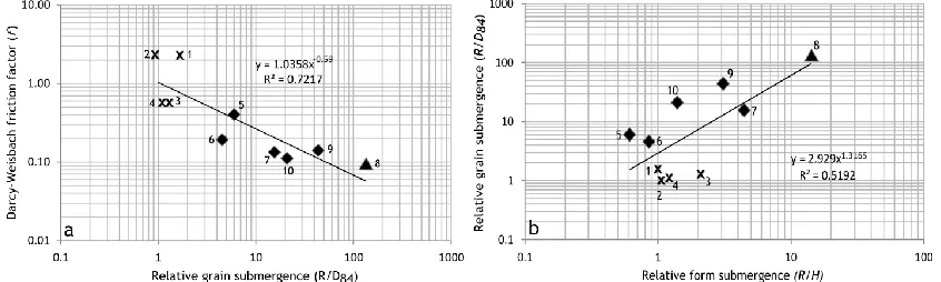
With a deformable boundary under certain discharge and sediment supply conditions, channel resistance is maximized by the topography of bedforms (Montgomery and Buffington, 1997; Wohl and Merritt, 2008). Relative grain submergence (R/D84)

increases downstream, i.e., grains protrude less into the flow and cause less resistance. Similarly, bedforms generate roughness that can be expressed by relative form

submergence (R/H). Wohl and Merritt (2008) present plots of Darcy-Weisbach friction factor (f ) versus R/D84that show no differences between values of f in pool-riffle vs.

step-pool channel types in response to increasing in R/D84. This suggests that bedform

roughness compensates for decreasing grain roughness (i.e. increasing R/D84)

downstream in mountain environments. The vertical dimension (H) of bedforms adjust to hydraulic variables (decreased slope, increased depth) so that R/H is consistent, ultimately minimizing the variance of hydraulic roughness in the downstream continuum from step-pool to pool-riffle channels (Wohl and Merritt, 2008)

However, the analysis of f and R/D84in this study reveals a statistically

significant (F=20.78, p=0.00186) decreasing trend in f (Figure 2.6a). This trend is consistent with trends observed in lower gradient channels (Knighton, 1998). The sequence of sites in this plot is generally consistent with a downstream trend except for the infilled site (8). Plots of R/D84and R/H also shows a systematic trend; R/H and R/D84

33

remain consistent as R/D84 increases. Figure 2.6 suggests that downstream bedforms

are not completely compensating for decreasing grain roughness.

Figure 2.6 Plots of Bedform Roughness. (a) Darcy-Weisbach friction factor versus R/D84 and (b) Relative grain submergence (R/D84) versus Relative form submerge (R/H).

Numbers represent downstream order of sample reaches. Bedform types symbolized as in Figure 2.5.

Rather, drastic decreases in gradient associated with the transition zone may be influencing downstream hydraulics so that complete compensation of bedform dimensions is unnecessary to achieve minimum variance in resistance.

The spatial locations of points in Figure 2.6 indicate that R/D84and R/H are not

34

35

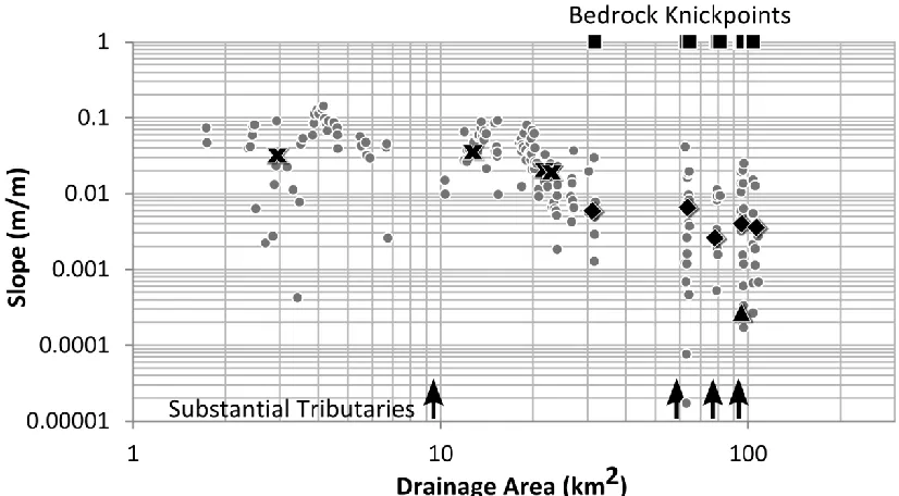
Figure 2.7 Slope-area Plot for Middle Saluda River (circles, background). Sample sites are symbolized as in Figure 2.6. Locations at drainage area are given for bedrock knickpoints (squares) and substantial tributaries (arrows).

highlights the great variability of channel gradients between tributaries—especially through the structurally controlled zone corresponding to bedrock knickpoints in the lower basin—and suggests the important role of slope in influencing bedform type. The variability in gradients in the lower basin is in contrast with the upper basin where channel gradients are less variable and show a stronger downstream decreasing trend below 10 km2.

2.6 D

C

2.6.1 KEY TRANSITION ZONE

36

channel change substantially

.

be identified at the watershed scale, analysis of hydraulic variables and bedforms suggests that local factors may explain the high variance embedded in these

relationships. The key transition zone is characterized by bedrock knickpoints as the river crosses structural ridges; substantial tributary inputs, one of which (Gap Creek) nearly doubles DA; substantial decreases in long profile slope but increases in slope variability; and increases in sand in the channel bed. Moreover, steep major tributaries meet the main channel near the inflection point of slopes (shown on Figures 2.4, 2.5, 2.7), causing substantial changes in discharge over a relatively short distance.

The data support the concept of a key transition zone in this study. Wohl (2004) hypothesizes a threshold of excess stream power (Ω/D84 = 10,000 kg/s3) at which

37

resistance measured by f, R/D84, and R/H (Figure 2.6) are also strongly influenced by the sample sites in the transition zone.

Slope may be the most critical variable in the key transition zone. The influence of forced gradients on mountain bedforms has been discussed (e.g. Thompson et al., 2006) but not yet explicitly tested. The key transition zone consists of six km of river punctuated by 17 erosion-resistant bedrock knickpoints as determined by a GPS field survey, with a central zone of greater density (2 km; n = 11) where the river cuts across a substantial ridge. While the influence of individual bedrock knickpoints is easily recognized in drastically forced morphologies at a specific stream reach (i.e. site 8), the structural control as a whole may be more broadly influential in that it can be viewed as a local baselevel control (Ferguson and Ashworth, 1991; Fryirs et al., 2007). Thus, sites 7 and 9, inside this structurally controlled zone, may be regarded as subtly forced

morphologies that are controlled by baselevel control of knickpoints, although their morphological changes are not drastic. This extends the definition of “forced” beyond the local reach-scale to the “macro-scale” (Thompson et al., 2006). Thus, the transition in bedforms may be a complex combination of the structurally forced decrease in gradient, individual steps in the longitudinal profile, and morphometrics of the watershed.

38

Fryirs et al., 2007), disturbance response (Montgomery and Buffington, 1997; 1998), and river restoration methods. Extended research could also focus on influences of

lithology, climate and hydrologic regime on the morphological transition of bedforms (Thompson et al., 2006).

2.6.2 CONCLUSION

The geomorphic transition of the Middle Saluda River from the Blue Ridge to the Piedmont provides an environment in which rapid fluvial changes in the downstream direction can be studied. Well-defined trends in DHG and bed material caliber were developed for the watershed and were compared with reach-scale bedform

39

suggest that DHG and downstream fining models should only be viewed as general trends and interpolation of fluvial characteristics from these generalizations should be applied with caution. Recognizing local changes in slope, bed material, and hydraulics should be emphasized when using downstream models of morphology for restoration or management objectives.

Acknowledgements: The authors would like to thank Ray Torres and John Kupfer for their input in the development of this project. Chris Kaase provided invaluable assistance with field work. The residents of Cleveland, South Carolina were also very helpful with field work.

2.7 R

40

CHAPTER 3

E

M

,

R

D

This chapter expounds upon the research where such details are not presented in the manuscript. The following sections include discussions of field data collection, analysis of hydraulic data, further results, and an extended discussion of implications.

3.1 E

M

3.1.1 LONGITUDINAL PROFILES AND CROSS-SECTIONS

41

and indicators of active flood deposits (USFS, 2008). Indicators were identified on both banks and marked with flags for surveying with a rod and level.

The range of terrain and channel morphology in the study resulted in different challenges to surveying each reach. Representative longitudinal profiles at two sites are presented here; the other profiles are given in Appendix B with cross-sections.

Longitudinal profiles for site 2 are shown in Figures 3.1 and 3.2. Linear functions of relative elevation (y) in terms of downstream distance (x) were determined by linear regression. Site 2 has a step-pool morphology with DA = 12.6 km2. The slope of the bankfull water surface (S = 0.038 m/m) (Figure 3.1) was used as an approximation of the slope of the energy grade line for computations of hydraulic parameters at this site. The morphology of the channel bed is indicated in Figure 3.2. Survey points were taken longitudinally in the thalweg to characterize bedform dimensions through the reach. Bedform amplitude (H) refers to the average difference in elevation between the crest of the step and the bottom of the pool. Wavelength (L) is horizontal measure of crest to crest or pool to pool. Often, both were calculated and averaged for wavelength.

Longitudinal profiles for site 7 (pool-riffle, DA = 79.2 km2) are shown in Figures 3.3 and 3.4. The long profile of bankfull water surface indicators at this site is an

example of the potentially complicated nature of identifying bankfull morphology in the field (Figure 3.3). Steep, heavily-vegetated banks made identification of bankfull

42

Figure 3.1 Longitudinal Profile of Bankfull Indicators – Site 2. The slope of this line is used as an estimate of the slope of the energy grade line.

Figure 3.2 Longitudinal Profile of the Channel Bed – Site 2. Bedform dimensions were calculated from this profile along the thalweg.

In this case, the slope of the channel bed was used for comparison (Figure 3.4). Channel bed slope was surveyed approximately twice the longitudinal distance as the bankfull indicators and gives a similar result (S = 0.0025 m/m). The slope of the energy grade line was estimated after taking both profiles into consideration. The channel thalweg

topographic survey was also used for pool-riffle bedform dimensions (Figure 3.4), and GPS points at pools were taken at downstream pool-riffle sites, such as site 7, where

y = -0.04x + 3.31 R² = 0.99

0 1 2 3 4 5

0 20 40 60 80

Rel ati ve El ev ati o n ( m)

Distance Downstream (m)

y = -0.04x + 4.42 R² = 0.84 0 1 2 3 4 5

0 20 40 60 80 100

Rel ati ve El e va ti o n ( m)

43

pools were highly spaced and morphology was consistent and uninterrupted. This was done so that bedform wavelength could be estimated beyond the surveyed reach.

Cross-section sites were chosen to be representative of the reach and conducive to surveying. Approximately 30 stations were surveyed for each cross-section with the intent to characterize the shape of the channel, banks, floodplain (if present) and valley where applicable. sections for each site are presented in Appendix B. Cross-sections were analyzed using a third-party spreadsheet program (NRCS, 2012), which requires stations (m), elevations (m), reach slope (S), and an estimation of Manning’s roughness coefficient (n). Roughness can be specified for each station or applied to parts of the cross-section (i.e. banks, channel, or floodplain). With this input, the program returns a suite of hydraulic variables associated with a range of stages.

44

bankfull indicators were marked in the field and recorded. The range of possible bankfull stages from the field were revisited in cross-section analysis after estimating roughness.

Figure 3.3 Longitudinal Profile of Bankfull Indicators – Site 7.

Figure 3.4 Longitudinal Profile of the Channel Bed – Site 7.

Consideration was given to estimating Manning’s n visually in the field, under the assumption that flow depths approximate bankfull stage. Barnes (1967) gives high and low measurements of roughness with photographs used for visual information. Further estimation of Manning’s n was computed using Jarrett’s (1984) empirical equation for steep channels (S > 0.002 m/m) for sites 1 – 6;

n = 0.39 S0.38R-0.16 (Eq. 6).

y = -0.00x + 1.18 R² = 0.04

0 0.5 1 1.5 2

0 10 20 30 40 50 60 70

Rel ati ve El ev ati o n ( m)

Distance Downstream (m)

y = -0.00x + 0.62 R² = 0.49

0 0.5 1 1.5 2

0 50 100 150 200

Rel ati ve El e va ti o n ( m)

45

Jarrett (1984) reports an average standard error of 28% for this equation versus measured values of n. In a comparison of methods for evaluating velocity in steep channels, Yochum et al. (2012) suggest that Jarrett’s equation has the least RMS error, though it is biased toward under-prediction in streams with higher roughness values. Estimating roughness at sites 1 and 2 utilized another empirical equation developed by Yochum et al. (2012), which can be applied to smaller, steep channels;

n = 0.41 ( ) (Eq. 7),

where is median maximum flow depth, taken from the longitudinal profile of the channel bed (m), and is the standard deviation of the residuals of the water surface

longitudinal profile (m). The median maximum flow depth can be visualized by superimposing the bankfull stage and bedform longitudinal profiles at a site (e.g., Figures 3.1 and 3.2). This method accounts for bedform dimensions (i.e. ) as the dominant influence of roughness and explicitly employs depth estimates from bankfull markers in the field.

The combination of visual estimates and empirical models produced a range of Manning’s n values for each cross-section. Sites 1 and 2 had higher ranges due

46

exemplified at site 5 where sinuosity contributed additional roughness. The ranges of values (Table A.2) were analyzed as inputs for the cross-section analysis. Finally, an iterative process of comparing calculated hydraulic geometry and discharge values with regional hydraulic geometry curves (Harmon et al., 2000) and gage data was

undertaken. Figure 3.5 is an example of a cross-section with multiple field estimates of bankfull stage (Site 3, DA = 21.7 km2). Channel morphology at this site is step-pool with S = 0.021 and D84 = 540. The methods above were applied to the cross-section, utilizing

Jarrett’s equation and visual estimation to estimate a Manning’s n value of 0.08. Hydraulic calculations using this value resulted in a bankfull stage estimation at the lowest field indicator.

Figure 3.5 Cross-section and Bankfull Estimation at Site 3. Dashed lines across the section, from bottom to top: water surface at survey, accepted low bankfull stage estimate, rejected medium bankfull stage estimate, rejected high bankfull stage estimate.

0 1 2 3 4

0 5 10 15 20 25 30 35

Rel

ati

ve

El

e

va

ti

o

n

(

m)

Station (m)

47

3.1.2 BED MATERIAL

Grid samples were collected from the coarsest surface layer of bed material

exposed in the reach at a spacing ranging between one and two meters, depending on the size of the bed material. The coarsest active bed material was sampled for each reach, representing bed material that exerts influence on channel morphology (Wilcock, 2001). Three additional bed material samples were collected in appropriate locations for better characterizing bed material around particular reaches (e.g. forced morphologies). The b-axis of each particle was measured in millimeters. Particle sizes representing D95,

D90, D75, D84, D50, D25, D16, D5 were calculated (mm) for each sample site using percentile

functions in R. Percentiles were converted to phi units (φ). Bed material statistics were calculated using the Folk and Ward (1957) graphical arithmetic measures (Bunte and Abt, 2001), including sorting, skewness, and kurtosis. Sorting, in this case, is related to standard deviation and is computed by;

𝛔 = ( ) (Eq. 8)

Skewness describes the symmetrical (or asymmetrical) nature of the distribution;

Sk = ₍ ( ) )

( )

( ) (Eq. 9),

and kurtosis refers to the peakedness;

K = ₍

48

Downstream trends in the statistics were explored and the results are presented in the next subsection.

Sand was visibly observed throughout the watershed. Highly-erodible grus contributes sand to the system from hillslopes in the upper watershed and tributaries throughout (Figure 3.6). In the Middle Saluda River, the areal coverage of sand

(particular in pools and bars) at the channel bed appears to increase downstream of site 5. The apparent increase downstream in sand coverage of the channel bed was sampled by probing transects across pools at pool-riffle reaches. The probe was thrust into loose sand until a clear refusal indicated contact with a coarser substrate and that depth was recorded.

49

3.2 E

R

3.2.1 BANKFULL DISCHARGE

Bankfull discharge (Qbkf) estimates were computed from approximate bankfull

cross-sections and estimated roughness. Qbkfestimates express a well-developed power

function relationship with drainage area (Figure 2.3). Further, Qbkfestimates in this study

are consistently greater (approximately 5%) than estimates generated from a regional curve (Harmon et al., 2000) at eight of ten sites. Sites 1 and 3, in the upper watershed, have slightly smaller Qbkf estimates compared to regional curves (4% and 0.2% smaller,

respectively). Qbkf at site 2, on the other hand, is 40% greater than predicted with the

regional curve. Inconsistencies in the upper watershed may reflect the low drainage areas represented by the low end of the regional model and the highly variable conditions typical of steep mountain channels. Further, it may reveal the difficulty of estimating discharge in high gradient streams, where slight increases in flow depth substantially increase discharge estimates. However, the iterative process by which Qbkf

was calculated lends confidence to the estimations in the upper watershed.

The apparently high estimates of Qbkf compared to the regional curve may be a

50

influenced climate patterns may result in bankfull flows of greater magnitude than other Southern Appalachian rivers in more western basins.

3.2.2 BED MATERIAL

Downstream fining of bed material is described well by an exponential model with R2 = 0.74 (Figure 2.4). This model excludes the uppermost sample because it occurs before substantial coarse sediment inputs. Folk and Ward (1957) graphical arithmetic statistics (Bunte and Abt, 2001) were calculated and classified for bed material samples. The reach at site 8 is an infilled morphology characterized by a sand bed that was not sampled with a surface grid, thus it does not have statistics. Patches of gravel at sites 8a and 8b, approximately 150 and 250 meters upstream, were sampled. These samples reveal a local fining of surface bed material at this forced reach (Table 3.1, Figure 3.8). Nine sites were poorly sorted, two were moderately well sorted and one was moderate. Nine sites are fine skewed or very fine skewed, one site is very coarse skewed and only two sites is considered nearly symmetrical. Sites 1-7 are considered leptokurtic (i.e. more peaked than a normal distribution). Sites 8a, 9 and 10 are platykurtic (less peaked) and site 8b is mesokurtic (normal). Given these non-normal descriptive statistics, further statistical analysis of bed material grain sizes would require methods robust to non-normal distributions.

51

52

Tables 3.1 Downstream Trends in Graphic Arithmetic Statistics Significance of ≤ 0.1 is in bold.

DA (km2)

σ Sk K

Intercept 1.5093 -0.2848 1.3727

Coefficient -0.0058 0.0026 -0.0041

R2 0.5781 0.2313 0.4301

F-statistic 13.7000 3.0090 7.5460

p-value 0.0041 0.1135 0.0206

Gradient (S)

σ Sk K

Intercept 1.0915 -0.0690 0.9952

Coefficient 12.2200 -6.4870 9.3559

R2 0.5360 0.3179 0.3038

F-statistic 7.0850 3.2630 3.0550

p-value 0.0249 0.1138 0.1240

Samples of the coarsest active bed material were included in this analysis for calculations of competency and a description of general downstream trends, but a total analysis of bed sediments would take into account the bimodality of surface bed

53

Figure 3.7 Trends in Graphic Arithmetic Statistics with Drainage Area

Figure 3.8 Trends in Graphic Arithmetic Statistics with Gradient

0.2 0.7 1.2 1.7

0 20 40 60 80 100 120

So rtin g ( σ )

Drainage Area (km2₎

-0.6 -0.4 -0.2 0.0 0.2 0.4 0.6

0 20 40 60 80 100 120

Skew n ess ( Sk )

Drainage Area (km2₎

0.4 0.6 0.8 1.0 1.2 1.4 1.6

0 20 40 60 80 100 120

Kurto

sis

(

K

)

Drainage Area (km2₎

54

3.3

E

D

Downstream trends in bed material, hydraulic geometry and bedforms are observed in the Middle Saluda River. Substantial changes in channel morphology appear to be associated with a key transition zone (Sections 2.5 and 2.6). One component of this transition zone is the drastic change in slope associated with structural ridges and bedrock knickpoints. The individual influence on channel morphology is evident at site 8, the infilled morphology. Slope is significantly reduced (Table A.2), depth increases substantially (Table A.2, Figure B.8), bed material caliber drastically decreases (Table A.3, Figure 2.4) and bedforms are replaced by a featureless sand bed. A conceptual longitudinal section of the reach is presented in Figure 3.9. Four transects were probed for depth of sand across the channel at the reach. Sand fill commences and increases downstream from an average depth of 14.5 cm to 111.5 cm. Local fining occurs on small gravel patches, which were grid sampled (Table A.3, sites 8a & 8b).

55

Figure 3.9 – Conceptual Longitudinal Profile of Infilled Morphology at Site 8

This is supported by Thompson et al. (2006)’s suggestion of macro-scale topographic influences on channel morphology and the observation that forced

morphologies typically have smaller bed material (Montgomery and Buffington, 1998). Further, alternating confined valleys and floodplain pockets, as observed in this study, have also been shown to be influential to sediment storage, disturbance response and channel processes (Magilligan, 1985; Fryirs and Brierly, 2010).

56

subsequently morphological, response to the key transition zone. This type of

morphology is not described in Wohl and Merritt (2008), which is a possible explanation for the differences between their plots of Darcy-Weisbach friction factor (f), relative form submergence (R/H) and relative grain submergence (R/D84) and the non-uniform

plots for this study (Figure 2.6).

Viewing the river as a large-scale forced morphology through the transition zone has implications for management and especially restoration. While it remains critical to assess hydraulic and sediment conditions at the reach scale, the location of the reach relative to landscape controls should be considered. This is especially true for

57

CONCLUSION

Downstream trends in hydraulic geometry (DHG), bed material and bedforms are observed in the Middle Saluda watershed, suggesting that downstream models can predict channel morphology at a broad scale. However, the limits of such models are indicated by the variability within the models. Understanding fluvial processes at a finer (and potentially more significant) scale requires the use of scale-independent methods, e.g. regime diagrams, that consider hydraulic and sediment data independent of

drainage area. This is especially important in mountain and transitional environments, where critical landscape controls of hydraulics and sediment are often highly variable. The Middle Saluda River is such an environment. The transition from the Blue Ridge to the Piedmont is characterized by a key transition zone consisting of substantial tributary inputs, structurally controlled gradients, alternating valley types and forced

morphologies. Data presented in this study suggest that landscape-scale features force channel morphology through the transition. The fluvial environment described in this study is different from those described in other studies of mountain stream morphology because of the rapid transition and the subsequent transition in bedforms. The data presented here offer new information for bed morphology in such an environment and add knowledge of a region that is lacking in fluvial geomorphic literature but is

58

REFERENCES

Abrahams, A. D., Li, G. and Atkinson, J.F. (1995) Step-pool Streams: Adjustment to Maximum Flow Resistance. Water Resources Research, Vol. 31, 2593–2602. Arcement, G.J. and Schneider, V.R. (1989) Guide for Selecting Manning’s Roughness

Coefficients for Natural Channels and Flood Plains. Washington, DC: U.S. Government Printing Office, U.S. Geological Survey Water-Supply Paper 2339 Barnes, H. H. (1967) Roughness Characteristics of Natural Channels. Washington, DC: U.S. Government Printing Office, U.S. Geological Survey Water-Supply Paper 1849.

Bernhardt, E.S., Sudduth, E.B., Palmer, M.A., Allan, J.D., Meyer, J.L., Alexander, G., Follastad-Shah, J. et al. (2007) Restoring Rivers One Reach at a Time: Results from a Survey of US River Restoration Practitioners. Restoration Ecology, Vol. 15, 482–493.

Best, J.L. (1988) Sediment Transport and Bed Morphology at River Channel Confluences. Sedimentology, Vol. 35, 481–498.

Blott, S.J. and Pye, K. (2001) GRADISTAT: a Grain Size Distribution and Statistics Package for the Analysis of Unconsolidated Sediments. Earth Surface Processes and Landforms, Vol. 26, 1237–1248.

Brummer, C.J., and Montgomery, D.R. (2003) Downstream Coarsening in Headwater Channels. Water Resources Research Vol. 39, 1294.

Buffington, J.M., Woodsmith, R.D., Booth, D.B., and Montgomery, D.R. (2003) Fluvial Processes in Puget Sound Rivers and the Pacific Northwest. In D.R. Montgomery, S. Bolton, DB Booth, and L. Wall, eds., Restoration of Puget Sound Rivers. Seattle, Washington: University of Washington Press, [46–78].

Bunte, K. and Abt, S.R. (2001) Sampling Surface and Subsurface Particle-size Distributions in Wadable Gravel-and Cobble-bed Streams for Analyses in Sediment Transport, Hydraulics, and Streambed Monitoring. Washington, DC: U.S. Government Printing Office, U.S. Forest Service General Technical Report RMRS-GTR-74.