Simple Waves characterizing wave propagation in a nonlinear elastic medium
Takao Momoi∗
(Received July 14, 1998; Revised April 13, 1999; Accepted April 14, 1999)
In the field of nonlinear waves, there exist two kinds of waves, i.e., one is Non-Coupled Simple Wave (nonlinear P wave) and Coupled Simple Wave (nonlinear S wave). In this paper, the problem is limitted to the two-dimensional case. After numerical computations, we have then found that the behavior of waves in the nonlinear wave field is governed by the theory of Simple Waves. Even complex wave form can be analyzed as composite Simple Waves.
1.
Introduction
In the previous papers (Momoi, 1990, 1992; these papers will be referred to papers A and B, respectively), we found two kinds of Simple Waves in a nonlinear elastic medium, that is to say, Non-Coupled Simple Wave (only a longitudinal component) and Coupled Simple Wave (a transverse compo-nent accompanied by a weak longitudinal compocompo-nent).
In order to clarify that these Simple Waves behave as domi-nant waves in nonlinear field, more intensive numerical com-putations was carried out in two-dimensonal case in this paper by use of the method in papers A and B. The behavior of the waves obtained is then explained by using the theory of Simple Waves.
2.
Simple Waves
In papers A and B, we have obtained expressions for Simple Waves. By use of second-order equations in two-dimensional case under new notations, these Simple Waves are described here in the case of an isotropic elastic medium as follows.
Let (x,z) be the components of Cartesian coordinates, (u, w)the displacement components of Simple Waves in the longitudinal (x-axis) and transverse (z-axis) direction, re-spectively,ta time variable,vpandvsthe velocities of linear P and S waves, respectively, and{λ,μ, A,B,C}the elastic constants. Furthermore, these elastic coefficients are nor-malized byμas follows.
Lm=λ/μ,Am= A/μ,
Bm=B/μ,Cm=C/μ.
(i) Non-Coupled Simple Wave
u =(2kr1Vp1)/g1, w=0, (1)
Vp1 =(vp2−vr12)/vs2, kr1=vr1t−x,
g1=6+2Am+6Bm+2Cm+3Lm,
wherevr1is a velocity of Non-Coupled Simple Wave.
∗2-25-3, Shakujiidai, Nerimaku, Tokyo, 177-0045, Japan.
Copy right cThe Society of Geomagnetism and Earth, Planetary and Space Sciences (SGEPSS); The Seismological Society of Japan; The Volcanological Society of Japan; The Geodetic Society of Japan; The Japanese Society for Planetary Sciences.
(ii) Coupled Simple Wave
u=(kr2Vs2)/f1,
w=sgw(kr2Wr1/2)/(f1vs), (2) Wr =Vs2(2v2p+v
2
s(−2+(2−g1/f1)Vs2)), Vs2=1−v2r2/vs2, kr2=vr2t−x,
f1=2+Am/2+Bm+Lm,
wherevr2 is a velocity of Coupled Simple Wave andsgwa
double sign±associated with the displacementw.
3.
Finite-Difference Equation
Leth be a unit length of the coordinate axesxandz. By use of the following expressions of time, coordinates and displacement components normalized byh,
ˆ
t=h·vpt, xˆ =h·x, zˆ=h·z,
ˆ
u=h·u, wˆ =h·w.
The governing equation is given by (refer to papers A and B)
∂uˆ/∂tˆ=U, ∂w/∂ˆ tˆ=W,
∂U/∂tˆ=T10+T11, ∂W/∂tˆ=T30+T31 (3)
with
T10 = ˆux2ˆ + ˆwxˆzˆLAM+(uˆˆz2vs2)/v2p,
T30 = ˆwˆz2+ ˆuxˆˆzLAM+(wˆx2ˆ vs2)/v2p,
and
T11 =(g1uˆxˆuˆx2ˆ +2f1uˆxˆzˆuˆˆz+ f1uˆxˆuˆˆz2
+2f2uˆxˆzˆwˆxˆ+ f2uˆˆzwˆx2ˆ + f1wˆxˆwˆx2ˆ
+f3uˆxˆwˆxˆzˆ+g2uˆx2ˆ wˆˆz+ f1uˆz2ˆ wˆˆz
+f3wˆxˆzˆwˆˆz+ f1uˆˆzwˆz2ˆ + f2wˆxˆwˆz2ˆ )(vs/vp)2, T31 =(f3uˆxˆuˆxˆzˆ+ f2uˆx2ˆ uˆˆz+ f1uˆˆzuˆz2ˆ
+f1uˆx2ˆ wˆxˆ+ f2uˆˆz2wˆxˆ+ f1uˆxˆwˆx2ˆ
+2f2uˆzˆwˆxˆˆz+2f1wˆxˆwˆxˆzˆ+ f3uˆxˆzˆwˆˆz
+f1wˆx2ˆ wˆzˆ+g2uˆxˆwˆˆz2+g1wˆˆzwˆz2ˆ )(vs/vp)2,
where
In order to solve the above equation by use of fi nite-differenece method, (uˆ,wˆ) and (U,W) are expanded by Taylor expansion up to the terms of second order with re-spect to time stepdtˆ(= ˆt− ˆt0) (refer to papers A and B). and velocity components at a timetˆandtˆ0, respectively, and other quantities with suffix 0 indicate the quantities at a time
ˆ
t0. The above method based on second-order expansion of Taylor series is much more stable and effective in conver-gence, so that the required time by this method is about a tenth of that by usualfirst-orderfinite-difference method.
After some reduction, the coefficients in (5) are expressed as tives given by (4) and these are replaced by the following difference equation.
ξxˆ =(ξ21−ξ01)/(2δh), ξzˆ=(ξ12−ξ10)/(2δh),
ξxˆ2=(ξ01+ξ21−2ξ11)/δh2,
ξzˆ2=(ξ10+ξ12−2ξ11)/δh2,
ξxˆzˆ=(ξ00+ξ22−ξ02−ξ20)/(4δh2),
where the numerical suffix in the above indicates a mesh point described in Fig. 1 andδh is a mesh interval normalized by h.
Fig. 1. Mesh points, wherehxandhzindicatexˆandˆz, respectively.
A stability problem of the computation always occurrs in the numerical computation by use of thefinite difference method. On the occasion of the numerical computation in the
linearequation, we can analyticallyfind a stability criterion
likeNeumancondition. In the case ofnonlinearequation,
such a treatment is impossible, so that the stabilty of the computation is confirmed by a lot of numerical trials of the computation. After such trials, the following values
dtˆ=0.1, δh =0.5
are confirmed to keep the numerical computation sufficiently stable.
4.
Initial Condition
The following expression for an initial condition is given near the wave origin.
ξ =(A(ξ)/2){1+cos(xˆπ/4)}, (6) (−4<xˆ<4) (forξ = ˆu,wˆ,UandW). Since we are treating the problem in two-dimension, a wave origin is like a mountain ridge.
5.
Numerical Experiment
The ability of a computer goes up more than that when the computation in papers A and B was carried out, so that new computation was made by use of more efficient computer. Then the values of elastic coefficients were specified as
5.1 Instance 1
In Fig. 2, the amplitudes in (6) are expressed as
A(uˆ)=0.2 and A(ξ)=0(ξ= ˆw, U, W).
The wave origin (6) with the above amplitude indicates that a push-type displacement is given at the origin in the direction of the wave propagation.
As found from Fig. 2, the positive side (push part) of the amplitude of the wave decreses with propagation, while, in due course, the negative side (pull part) increases. Each wave form of these waves is a pulse of triangular type instead of a sinusoidal one, and further propagated at a velocity near linear P wave (not exact P wave velocity). The above exposed results are very important together with those in the next numerical instance.
In the figure, hx and hu-axes indicate normalized dis-tancehx = ˆxand normalized displacement multiplied with ‘Vertical scale’ (described on the top of the figure), i.e., hu=(Vertical scale)× ˆu. Thefirst (leftmost) broken line is that attˆ=0 (initial value). The other broken lines indicate wave forms by step time 50 and the bold solid line afinal wave form, which is that attˆ = 500 in this case, respec-tively. These conventions except the last one associated with the time of the last wave form follow in the same way in the subsequent Figs. 3, 5, 6, 7 and 8.
In Fig. 3, the amplitudes in (6) are expressed as
A(uˆ)= −0.2 and A(ξ)=0(ξ = ˆw, U, W).
The wave origin (6) with the above amplitude indicates that a pull-type displacement is given at the origin in the direction of the wave propagation.
As found from Fig. 3, the pull-type wave at the wave ori-gin is propagated by holding a pull-type feature at a velocity
Fig. 2. Propagation of Non-Coupled Simple Wave in the case of positive initial displacement of wave origin.
Fig. 3. Propagation of Non-Coupled Simple Wave in the case of negative initial displacement of wave origin, where hx = ˆx and
hu= (Vertical scale)× ˆu. Thefinal wave form (bold line) is that at ˆ
t=500.
near linear P wave. As propagating, the width of the wave becomes wider by changing the wave form into a trapezoidal one. The wave shown in Figs. 2 and 3 will be named nonlin-earP wave later on.
Let us explain the above-mentioned two features such that the push-type nonlinear P wave pulse (Fig. 2) becomes nar-rower in a triangular form and the pull-type nonlinear P wave pulse (Fig. 3) becomes wider in a trapezoidal form.
Weassumethat these waves consist of a few fragments of
Simple Waves described in Section 2. Though we use a term of‘assume’in here, all numerical experiments indicate that this assumption is not only an assumption, but a truth itself. Suppose that Non-Coupled Simple (nonlinear P) Waves in Section 2 constitute the waves exposed in Figs. 2 and 3. We can put
vr1=vp+dvp(dvp: a small quantity) (7)
in (1). By taking the term up tofirst order ofdvp, we obtain
u=(−4dvpvp(vr1t−x))/(g1v2s), (8)
The expressions (7) and (8) indicate very important facts such that
(i) when the wave front (fragment of Non-Coupled Sim-ple Wave) is propagated at a velocity f ast er than that of linear P wave (dvp>0), the wave front is of a pull-type (u decreases).
(ii) when the wave front is propagated at a velocityslower than that of linear P wave (dvp <0), the wave front is of a
push-type (uincreases).
(9)
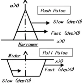
Let us consider a triangular or trapezoidal pulse of a wave composed of two push and pull Non-Coupled Simple Waves. As shown in Fig. 4, very interesting features are found from (i) and (ii) in (9). In this figure, lines with arrowSlowor Fast indicate wave fronts (Simple Waves) of a pulse which moves at a velocitysloweror f ast er than that of linear P wave, respectively.
Two features in (9) leads to very interesting features such that
(i) a triangular pushpulse (topfigure) becomes narrower with the propagation,
(ii) a triangularpullpulse (bottomfigure) becomes wider with the propagation and tends to a trapezoidal form.
(10)
By use of the theoretical model mentioned above, the result of numerical experiments (Figs. 2 and 3) will be elucidated again. The phenomenon such that the push wave becomes smaller in a triangular form with the propagation (Fig. 2) can be explained by the top model in Fig. 4, while the phe-nomenon such that the pull wave becomes wider in a trape-zoidal form with the propagation (Fig. 3) can be explained by the bottom model in Fig. 4.
In the linear theory, a trapezoidal wave like that in Fig. 3 is named asat ur at edwave. On the occasion of the nonlin-ear theory, the termsaturated waveis not appropriate, since the generation process of the trapezoidal wave is completely irrespective of a saturation process.
Let us make mention of the advancing velocity of Coupled Simple Wave in here. Like the case of Non-Coupled Simple Wave, we put
vr2=vs+dvs(dvs: a small quantity) (11)
Substituting the above into (2) and taking the term up to first-order ofdvs, we have
In the above expression, the displacement componentwhas a factor(−dvs)1/2, so thatdvsis required to be negative in order for the componentwto exist (square root is required to be real). In due course, Coupled Simple Wave is always propagated at a velocity less than that of linear S wave from (11). Furthermore, the longitudinalu-component (∼ |dvs|) is smaller in quantitiy than the transversew-component (∼
|dvs|1/2).
Some comment is made, in here, on the wave form like that appeared in Fig. 2. Such an oscillatory wave form is frequently found on the occasion of large earthquake. If the interpretation of the wave form like that is done based on a linear theory, the wave source is interpreted to be of an oscillatory type. If a nonlinear process occurs both near the wave source and during the propagation process, this interpretation based on a linear theory is completely wrong from the result in Fig. 2.
5.2 Instance 2
Figure 5 is an instance where the amplitude in the expres-sion (6) is given by
A(U)=0.2 and A(ξ)=0(ξ = ˆu, w,ˆ W).
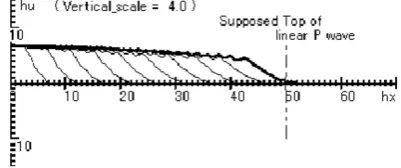
This expression indicates the case where a push veloc-ity is given at the wave origin in the direction of the wave propagation. In this case, a push-type step wave appears in thefigure, the height of which decreases gradually with the propagation. The front of the generated wave is a push-type Simple Wave and the top of the wave is propagated at a ve-locity slower than that of linear P wave as expected from (ii)
Fig. 5. Propagation of Non-Coupled Simple Wave in the case of positive ini-tial velocity of wave origin, wherehx= ˆxandhu=(Vertical scale)× ˆu. Thefinal wave form (bold line) is that atˆt=500.
Fig. 6. Propagation of Non-Coupled Simple Wave in the case of negative ini-tial velocity of wave origin, wherehx= ˆxandhu=(Vertical scale)× ˆu. Thefinal wave form (bold line) is that atˆt=500.
in (9). In thefigure,‘Supposed Top. . .’indicates an apex of a linear triangular P wave instead of a rightward foremost head.
Figure 6 is an instance where the amplitude in the expres-sion (6) is given by
A(U)= −0.2 and A(ξ)=0(ξ = ˆu, w,ˆ W).
This expression indicates the case where a pull velocity is given at the wave origin in the direction of the wave prop-agation. In this case, a pull-type step wave appears in the figure. The wave front is a pull-type Simple Wave and the top of the wave is propagated at a velocity faster than that of linear P wave as expected from (i) in (9). In the part of the wave front, the dispersion of the wave (several steps) occurs in such a way that the foremost head part (steep gradient) is more accelerated than the later part (gentle gradient). This feature is explained as follows.
From (7) and (8), it is found that, if the gradient of u is steeper (larger),dvp is also larger (from (8)), so that the velocity of the wave becomes faster (from (7)).
5.3 Instance 3
Figure 7 is an instance where the amplitude in the expres-sion (6) is given by
A(w)ˆ =0.2 and A(ξ)=0(ξ = ˆu, U, W).
Fig. 7. Propagation of Coupled Simple Wave in the case of positive initial displacement of wave origin in the transverse direction, wherehx = ˆx
andhw=(Vertical scale)× ˆw. Thefinal wave form (bold line) is that attˆ=1000.
Fig. 8. Propagation of Coupled Simple Wave in the case of positive initial velocity of wave origin in the transverse direction, wherehx = ˆxand
hw=(Vertical scale)× ˆw. Thefinal wave form (bold line) is that at ˆ
t=1000.
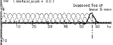
Figure 8 is an instance where the amplitude in the expres-sion (6) is given by
A(W)=0.2 and A(ξ)=0(ξ= ˆu, w,ˆ U).
This expression indicates the case where an initial velocity
is given at the wave origin in the transverse direction of the wave propagation. In this case, a wave front of Coupled Simple Wave appears at the head of the wave.
In Figs. 7 and 8, the top of Coupled Simple Wave is prop-agated at a velocity a little slower than that of linear S wave as discussed in (11) and (12), so that Coupled Simple Wave is namednonli nearS wave.
6.
Conclusion
In this study, we have found a very impotant fact such that the propagation of nonlinear waves is fundamentally gov-erned by the theory of Simple Waves. Even oscillatory com-plex waves can be analyzed as waves consisting of several fragments of Simple Waves. This fact has an important sig-nificance in such a way that on the occasion of the response evaluation of nonlinear waves at the boundary we can as-sume, as the first approximation, the incident and reflected nonlinear waves to be a congregation of Simple Waves. By using nonlinear stress boundary conditions and the above Simple Waves, we can analyze the temporary behavior of nonlinear waves near the boundary at a certain moment.
Another important exposed fact is such that nonlinear push P pulse becomes narrower in a triangular form with the prop-agation, while nonlinear pull P pulse becomes wider in a trapezoidal form with the propagation.
References
Momoi, T., Wave propagation in nonlinear-elastic isotropic media, Bull. Earthq. Res. Inst.,65, 413–432, 1990.
Momoi, T., The polarization of waves in an anisotropic nonlinear-elastic medium,Bull. Earthq. Res. Inst.,67, 1–20, 1992.