Time dependency of fluid flow near the top of the core

(1)

Earth Planets Space,50, 813–825, 1998

Time dependency of fluid flow near the top of the core

A. Bhattacharyya

Indian Institute of Geomagnetism, Colaba, Mumbai 400 005, India

(Received October 24, 1997; Revised June 26, 1998; Accepted July 16, 1998)

Fluid flow in the core is assumed to consist of a slowly varying (on time scales>magnetic diffusion time) part and a smaller, rapidly varying part as in the theory of the hydromagnetic dynamo put forward by Braginsky (1965). On the basis of this theory, geomagnetic secular variation models for the last 150 years are used to determine a rapidly varying, axisymmetric, poloidal motion of the fluid near the top of the core as a function of latitude in regions away from the equator. Approximations made in estimating this motion fail near the equator, thus restricting the estimates to latitudes≥40◦. Amplitude of the oscillating part of the axisymmetric poloidal flow is found to be≤1 km/yr in the northern hemisphere, and nearly 3 km/yr in some parts of the southern hemisphere. The nature of temporal variation of this component differs significantly between the northern and southern hemispheres during the period under consideration.

1. Introduction

Time-dependent maps of the magnetic field at the core-mantle boundary (CMB) have been constructed by Bloxham and Jackson (1992) (hereinafter BJ92) using most of the available data for the last three centuries, and assum-ing the mantle to be an insulator. The spatial variation of the magnetic field is described in terms of spherical harmonics in the usual way, while its temporal variation has been rep-resented using a cubic B-spline basis. A secular variation model of the magnetic field at the CMB is thus available for the last 300 years.

Fluid flow in the outer core together with magnetic diffu-sion gives rise to temporal variation of the magnetic field at the CMB. Over time scales much shorter than the magnetic diffusion time associated with length scales ≥ few thou-sands of kilometers, the core may be considered to behave like a perfect conductor, such that the magnetic field lines are frozen in the fluid (Roberts and Scott, 1965). This argu-ment has been used by a number of workers to estimate large scale fluid flow near the top of the core from secular variation models at the CMB (Whaler, 1980; Gubbins, 1982; Voorhies and Backus, 1985; Backus and Le Mou¨el, 1986; Lloyd and Gubbins, 1990; Bloxham and Jackson, 1991). Apart from the frozen-flux approximation the above estimates required some other assumption about the fluid flow in order to overcome the problem of non-uniqueness inherent in the determination of fluid flow near the top of the core from the induction equa-tion (Backus, 1968). Hence the flow was considered to be either steady or geostrophic or toroidal in order to determine it uniquely from the frozen-flux induction equation.

In another approach (Rikitake, 1967; Honkura and

Rikitake, 1972; Honkura and Matsushima, 1988;

Matsushima and Honkura, 1989) to estimation of fluid flow in the outer core from a geomagnetic field model, it was

as-Copy right cThe Society of Geomagnetism and Earth, Planetary and Space Sciences (SGEPSS); The Seismological Society of Japan; The Volcanological Society of Japan; The Geodetic Society of Japan; The Japanese Society for Planetary Sciences.

sumed that the non-axisymmetric poloidal magnetic field is maintained against Ohmic diffusion by the interaction be-tween a strong zonal toroidal magnetic field and large-scale non-axisym-metric poloidal velocity fields as in anαω-type geodynamo. The strong zonal toroidal field was considered to arise from the distortion of a large scale axisymmetric poloidal magnetic field by differential rotation, which is the so calledω-effect. Rikitake (1967) and Honkura and Rikitake (1972) further assumed that non-zonal poloidal magnetic field of various modes and the toroidal magnetic field are in a steady state. These authors considered the representation of the non-zonal field in terms of standing and drifting parts sug-gested by Yukutake and Tachinaka (1969), and treated these two parts separately. Matsushima and Honkura (1988) ex-pressed the scalar potential describing the observed poloidal field in terms of standing and drifting parts with periodically varying amplitudes, which was then used by Honkura and Matsushima (1988) to estimate fluid motion in the core at different epochs at 100 year intervals from 1600 to 2000, by the same method as Honkura and Rikitake (1972). The con-vection pattern was found to vary from one epoch to another. It was pointed out by Matsushima and Honkura (1992) that theω-effect may not be as strong as was assumed in the earlier papers, so that it is necessary to consider the other interac-tion terms also in the inducinterac-tion equainterac-tion. Matsushima (1993) solved the induction equations for the toroidal and poloidal magnetic fields together with the Navier-Stokes equation for the toroidal velocity field to estimate fluid motion in the Earth’s outer core from a geomagnetic field model. The au-thor prescribed the radial dependence of the poloidal velocity field and minimized the temporal variations of the velocity and the magnetic fields. Thus at any particular epoch, the time derivative of the magnetic field at the CMB calculated using the velocity field derived by Matsushima (1993) was much smaller than given by the secular variation model for that epoch. Since secular variation of the poloidal field at the CMB contains important information about the geodynamo,

(2)

814 A. BHATTACHARYYA: TIME DEPENDENCY OF FLUID FLOW

it is necessary to consider it in attempts to estimate the tem-poral evolution offluidflow in the outer core, which would shed light on the existence of lateral temperature variations at the base of the mantle.

A time-dependent geomagneticfield model was used by Benton and Celaya (1991) to determine a unique, unsteady surfaceflow at some chosen points on the CMB, under the frozen-flux approximation, by considering the temporal evo-lution of thefluidflow to be quartic. They found that at one illustrative point on the CMB, an exactfit to the 1900–1980 field model of Bloxham and Jackson (1989) required consid-erable evolution of theflow. Hulotet al.(1993) were thefirst to show clearly that coreflows are highly time-dependent. This paper also gave thefirst account of a definite relationship of geomagnetic“jerks”with time-varyingflow in the outer core. More recently, Jackson (1997) has obtained models of time-dependent core surface motions for the period 1840– 1990, using time-dependent maps of the magneticfield at the CMB (BJ92) and the frozen-flux and tangentially geostrophic flow approximations.

Fluidflow in the core is expected to show variations on short time scales because changes in the length of day (LOD) on decadal time scales are usually associated with changes of angular momentum of the core (Jaultet al., 1988; Jackson et al., 1993). Further, Jackson (1997) has demonstrated in a forward calculation, that with steady motion of thefluid near the top of the core, it is not possible tofit the secular variation recorded at observatories to the required level of accuracy, even on short time scales of a few years. In the present paper, a method put forward by Bhattacharyya (1995), to use the secular variation of the axisymmetric poloidal magnetic field at the CMB to determine a rapidly oscillating (on time scalesmagnetic diffusion time) part of the axisymmetric meridionalflow near the top of the core, is utilized to study the temporal evolution of this component of surficial core flow over the period 1840–1990.

2. Geodynamo Model

A geodynamo model in which time variations of the mag-neticfield andfluidflow in the outer core are built in, is the hydromagnetic dynamo model of Braginsky (1965). In this model, the non-axisymmetric partUof thefluidflow in the core is considered to be a superposition of waves propagating in theφ-direction, and the axially symmetric part of theflow is assumed to consist of a slowly varying (∂/∂t ≈ ηc−2, where η is magnetic diffusivity and c is the core radius) part and a rapidly oscillating partU˜. This rapidly oscillat-ing axisymmetricflow was termed oscillations by Braginsky (1965). The outer corefluid motion is thus expressed as:

Utot=Uφˆ+UP+ ˜U+U (1)

whereUφˆandUPare the toroidal and poloidal components

of the slowly varying axisymmetric part of theflow,φˆbeing a unit vector in the azimuthal direction. Braginsky (1965) assumed that for a nearly axisymmetric dynamo,Uˆ ≈U≈ U R−m1/2, whereRm 1 is the magnetic Reynolds number

defined by Rm =UMc/η,UMbeing a typical value ofU. It

was also assumed in this model that the slowly varying ax-isymmetric part of theflow is dominated by the toroidalflow andUP≈U Rm−1. With the assumption of large scale, slowly

varying velocity and magnetic fields, Matsushima (1993) had found the toroidal velocity to be dominant at the CMB. In Braginsky’s (1965) hydromagnetic dynamo the magnetic field was also represented in a manner similar to the velocity field:

Btot=Bφˆ+BP+ ˜B+B. (2)

The mantle is assumed to be an insulator such that at the top of the core,B=0 andB˜_φ=0. Also the CMB is assumed to be a free-slip, spherical boundary, such thatUr = ˜Ur =Ur=0 atr =c, whereUr,U˜r, andUrare the radial components of

UP,U˜ andUrespectively.

Under these conditions, Braginsky (1965) found that for the time-varying axisymmetric poloidalfieldB˜P, which can

be expressed in terms of a vector potential A˜φˆ:

˜

BP= ∇ ×(A˜φ),ˆ (3)

only oscillations of thefield of order Rm−3/2 can pass to the

outside of thefluid core, and these are determined by

∂A˜

∂t =[U˜P×BP]φ. (4)

Consideration of the momentum equations governingU˜ and UPby Bhattacharyya (1995) showed that a term proportional

toUPalso makes a contribution to ∂B˜P/∂t at the CMB of

the same order, and hence must be included to obtain the following equation for its radial component:

∂B˜r where the z-axis is along the Earth’s rotation axis and Br is the radial component of the slowly varying, axisymmet-ric poloidal field BP. Determination of fluid flow at the

top of the core from the radial component of the classical frozen-flux induction equation suffers from the problem of non-uniqueness because it involves solving a single scalar equation for a two-dimensional vectorflow. Equation (5) is derived from the longitudinally averaged radial component of the frozen-flux induction equation, and the problem is now reduced to solving this equation to determine a single scalar. Hence it is possible to obtain an unique solution as has been demonstrated by Bhattacharyya (1995).

The left-hand side of Eq. (5) may be expressed in terms of spherical harmonics:

n(t)is thefirst derivative with respect to time of the Gauss coefficientg0

(3)

A. BHATTACHARYYA: TIME DEPENDENCY OF FLUID FLOW 815

Fig. 1. Radial componentBr of a steady, axisymmetric poloidal magneticfield at the CMB as a function of colatitude, derived from the time average normal-polarity palaeomagneticfield model of Kelly and Gubbins (1997).

Thefirst term involving E0 is independent ofθ and is

de-termined by the condition that on the CMB, at θ = 0 (or

θ=π),U˜z= ˜Ur =0 andUz=Ur =0: axisymmetric parts of the Navier-Stokes equation, under the Boussinesq and magnetostrophic approximations, were also used by Bhattacharyya (1995) to show that the contribution of the second term on the left hand side of Eq. (7) equals that of thefirst term. Thus the following solution is obtained for

˜

3. Fluctuations in Axisymmetric Poloidal Flow

For the period 1840–1990, the Gauss coefficients for the expansion of the time rate-of-change of the geomagnetic field, in terms of spherical harmonics upto N = 14, are available from the time-dependent models of the magnetic

field at the CMB obtained in BJ92. These are used to com-pute the coefficientsEn(t)for various epochs. The slowly varying component Br is, as such, an unknown in the calcu-lation ofU˜z from Eq. (10). However, it should be borne in mind that, at a given co-latitudeθ, by definitionBrshould not vary over a time-period of 150 years. Hence the short-period fluctuations inU˜z are determined entirely by the numerator of Eq. (10). Thus conclusions drawn from Eq. (10) regard-ing the pattern of short-period variations in the axisymmetric poloidalflow will not be affected by the choice ofBr except in those regions where Br is so small as to invalidate the approximations that go into the derivation of Eq. (10) which involves neglect of higher order terms. This happens in the neighbourhood of the geographic equator where the radial component,Br, of the axisymmetric part of the geomagnetic

field is small. For the estimation ofU˜z from Eq. (10), Br has been calculated from the axisymmetric part of the time-average palaeomagneticfield obtained by Kelly and Gubbins (1997). These authors used directional measurements from lavas, inclination measurements from ocean sediments and intensity measurements from lavas to arrive at geomagnetic field models for the past 5 Myr. The time-average normal-polarity palaeomagneticfield model obtained by Kelly and Gubbins is not axially symmetric, but the axisymmetric part is dominant. The radial component of the axisymmetric part which is used as Br in the present study is shown in Fig. 1. For reasons stated above, estimation of U˜z from Eq. (10) using thisBris restricted to latitudes≥40◦.

(4)

us-816 A. BHATTACHARYYA: TIME DEPENDENCY OF FLUID FLOW

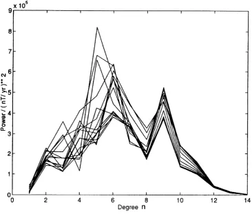
Fig. 2. Secular variation power at the CMB, calculated from the time-dependent geomagneticfield model BJ92 as a function of the harmonic degreen, for each decade of the period 1840–1990.

ing Eq. (10) is the truncation levelN. The secular variation power at the CMB, calculated from the time-dependent geo-magneticfield model of BJ92 for each decade of the period 1840–1990, is plotted in Fig. 2 as a function of the harmonic degreen. This includes the non-axisymmetric part as well. An interesting feature that is revealed by this plot is the vari-ability of the spectrum of the secular variation upto degree n =6, from one decade to another. It is seen that the peak in the power atn =9 emerges as a more stable feature dur-ing this period. This is mainly controlled by the regularisdur-ing procedure used in obtaining the BJ92 model, which is based on the smoothest solutions compatible with the observations. This procedure involved minimization of two model norms, measuring roughness in the spatial and temporal domains re-spectively, and this is expected to result in greater stability for degrees higher than 7 or 8. Secular variation of the geomag-neticfield at the CMB has contributions from bothfluidflow and magnetic diffusion, the latter contributing much more towards the temporal evolution of small scale features of the magneticfield than to the large scale features. Thus the tem-poral variability of the secular variation atn ≤ 6 may be a direct manifestation of the temporal variability offluidflow in the outer core. By this argument it may be sufficient to consider a truncation levelN =6 for estimating the tempo-ral evolution offluidflow near the CMB. Nevertheless, for checking the convergence of the results, truncation levels of N =8 andN =14 have also been used in the calculations.

At the CMB, the meridional component U˜_θ of U˜P can

be determined from U˜z because the radial component U˜r vanishes there, yielding

˜

U_θ = − ˜Uz/sinθ. (11)

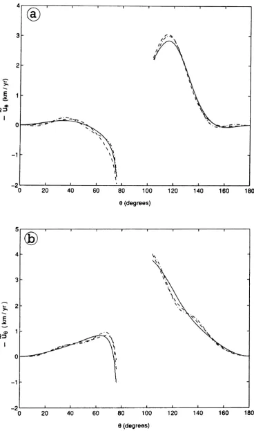
At the poles (θ =0◦, 180◦),U˜θmust be zero in order to be physically defined. This should be automatically satisfied by the solution obtained for U˜_θ from Eq. (11). SinceU˜z vanishes at the poles according to the boundary conditions used in obtaining the solution Eq. (10), l’Hospital’s rule has to be applied to Eq. (11) to demonstrate explicitly thatU˜_θalso vanishes at the poles. Plots ofU˜_θas a function ofθ for the epochs 1900 and 1960 are shown in Fig. 3 forN =6, 8 and 14. It appears that increasingNfrom 6 to 14 does not change the estimates drastically. A breakdown in the validity of the approximations leading to Eq. (10) explains the unphysically large values ofU˜_θin the neighbourhood of Br =0, where there is a discontinuity inU˜zas given by Eq. (10). Retention of higher order terms would remove such a discontinuity in

˜

(5)

(6)

(7)

(8)

Fig. 4. (continued).

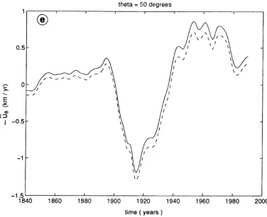
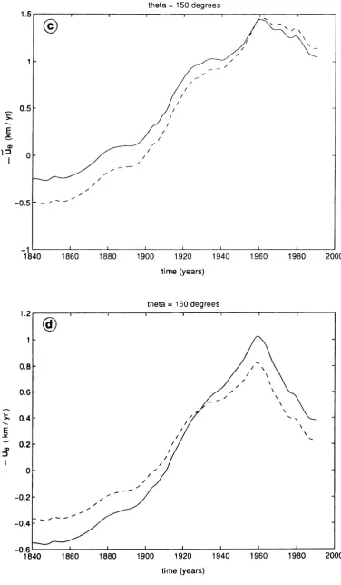
However, it can not be claimed that this is the correct bound. It is a non-controversial bound as far as a comparison between the two hemispheres is concerned. An estimate of the higher order corrections could yield a lower cutoff value ofθ for which the computed values ofU˜_θmay still be considered as reliable. In fact, a comparison of Figs. 3(a) and (b) shows more pronounced differences between epochs 1900 and 1960 for colatitudes belowθ=130◦, which can not be attributed to Br. The choice ofθ = 50◦ as the upper bound in the northern hemisphere is on the basis of Fig. 3(a), since for values ofθ >60◦the estimates ofU˜_θ appear to be affected by the singularity in the vicinity ofθ = 80◦. Once again, a quantitative estimate of the cutoff has not been given, and the present choice may be an underestimate of the correct one. The main contention here is the difference between the patterns of temporal evolution ofU˜θin the two hemispheres, which is not directly affected by the magnitude ofBr at the higher latitudes. This is studied at selected latitudes for the 150 year period extending from 1840 to 1990, using the time-dependent secular variation model of BJ92. The results for northern and southern latitudes are shown in Figs. 4 and 5 respectively. Once againU˜_θcomputed both withN =6 and N =14 are shown in thesefigures.

It will be recalled that the diffusion term itself was ne-glected in arriving at Eq. (4), as a consequence of the assump-tion that Rm 1. However in the estimated coefficients

˙ gm

n for the secular variation of a time-dependent geomag-netic field model derived from observations, the contribu-tion from diffusion is included. The smaller the length scale

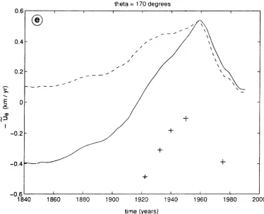
of the magneticfield, the more the magneticfield diffuses, hence there may be greater contributions from diffusion to the secular variation coefficients for higher degrees, and the temporal evolution of the secular variation coefficients g˙nm forn >6 could be such as to make the temporal variation of the computedU˜_θ significantly different for N = 6 and N =14. However, it appears from Figs. 4 and 5 that, except atθ =170◦, at the other colatitudes shown in thesefigures, temporal variation of the computedU˜_θis not very different for N =6 andN =14. To check the sensitivity of the nu-merical method at different latitudes,five different models of secular variation listed in table 16 of Langel (1987) for epochs 1922.5, 1932.5, 1940, 1950 and 1975, are used to calculateU˜_θ atθ = 10◦ andθ = 170◦. These values are shown by crosses on Figs. 4(a) and 5(e) respectively. For epochs 1922.5 and 1932.5 the models have a truncation level ofN =6 whereas for epochs 1940, 1950 and 1975 the mod-els are truncated at N =8. Although the magnitude ofBr atθ =170◦ is greater than that atθ =10◦, the results at

θ = 170◦ are much more sensitive to the model used and hence do not appear to be reliable.

4. Discussion

(9)

(10)

(11)

Fig. 5. (continued).

scales on which thisfluidflow shows variations at differ-ent latitudes and to approximately estimate the magnitude of suchfluctuations. In his theory of the hydromagnetic dy-namo, Braginsky (I965) considered the non-axisymmetric part of the velocity to arise from a superposition of waves travelling in theφ-direction. The basis for this was stated to be the observation that the geomagneticfield undergoes sec-ular variations in which the non-axisymmetric components tend to drift predominantly towards the west, with different velocities. However, the axisymmetric part of the geomag-neticfield also has a small component varying on“fast”time scales which are much shorter than the magnetic diffusion timec2_/η_{. Hence, Braginsky (1965) introduced the}

con-cept of “oscillations”which represent a rapidly oscillating component of the axially symmetric velocity that contains a slowly varying (on time scales≥c2_/η_{) part as well. The}

poloidal part of this axisymmetric oscillatory motion may be written as

˜ UP=

μ

u_μexp−iφμ ₍₁₂₎

where the amplitudesu_μand the frequenciesφ˙_μare assumed to have a slow time variation, so that the phasesφ_μof the oscillations are almost linear functions of time (Braginsky, 1965). An axisymmetric, poloidalflow would have onlyr -andθ-components, of which ther-component vanishes at the top of the core. HenceU˜_θ defines the axisymmetric, os-cillatory component of the poloidalflow and a study of its temporal evolution is expected to give an idea of the frequen-ciesφ˙_μ involved. Estimates ofU˜_θin the present study, are

usedfirstly to check the validity of the description provided by Eq. (12). Braginsky’s (1965) theory requires thatU˜P

av-eraged over a period of time>c2/ηshould yield zero. Even for the short duration of 150 years studied here, a tendency towards such oscillatory behaviour, with periods less than 150 years, is seen atθ≤50◦in the northern hemisphere and

θ ≥150◦in the southern hemisphere, since at these latitudes ˜

U_θchanges sign in the course of these 150 years. However atθ =130◦ andθ = 140◦ longer period oscillations also seem to be present which would require a longer data set to be studied. Nevertheless, even at these latitudes short period oscillations are seen, modulated by the longer period oscilla-tions. With a sufficiently long time series, a Fourier analysis could be carried out to determine the frequencies, which is not feasible in the present study.

(12)

of day (LOD) thatfluctuations in core surfaceflow is about ±1 km/yr. This calculation was for a mean westwardflow near the core surface.

Further differences in the temporal variation offluidflow near the CMB in the two hemispheres is evident from Figs. 4 and 5. The axisymmetric meridionalflow near the CMB shows greater variability on short time scales or“jerk”-like behaviour in the northern hemisphere than in the southern hemisphere. In the northern hemisphere for 20◦≤θ≤50◦, there is rapid variation in this component of theflow close to 1895, 1915 and 1970. Global rms value of secular vari-ation in the radial component of the geomagnetic field at the earth’s surface derived from model ufm1 of BJ92 dis-plays the phenomena of“jerks”as can be seen infigure 1b of Jackson (1997), whereas the global rms value of secu-lar variation in the same component at the CMB, derived from the same model, shows much smoother variation with time as infigure 1c of Jackson (1997). However, present re-sults indicate that large scalefluidflow near the CMB shows more complex temporal behaviour than the geomagneticfield at least in the northern hemisphere. In the southern hemi-sphere, forθ≥150◦, there is a sharp change in the axisym-metric meridionalflow close to the 1960 epoch only. For 130◦ ≤θ≤140◦, the temporal variation of this component of theflow is quite different showing oscillatory behaviour with a period of about 60 years superimposed on longer pe-riod variations.

In this paper, no attempt is made to estimate the time vari-ation of the zonal toroidalflow. Hence the results obtained here cannot be directly compared with the root mean square velocity at the CMB or the zonal toroidal rms velocity over the CMB, estimated as a function of time by Jackson (1997) using the time-dependent field model ufm1 of BJ92. The flows derived in that work are the simplest in a spatial and temporal sense, while being compatible with the mainfield and secular variation values provided by the model ufm1 of BJ92. Thus, all the short time scale variations seen in some of thefluidflows obtained in the present work are not expected to be seen in Jackson’s (1997) results. Nevertheless, both the root mean square velocity and the zonal toroidal rms velocity at the CMB obtained by Jackson (1997) show sharp peaks near the 1915 epoch. The earlier paper by Hulotet al.(1993) has also discussed such peaks in the outer corefluidflow near the 1915 epoch. The present results have no contribution to-wards changes in LOD, and hence cannot be compared with LOD observations as such. It may simply be argued that whatever phenomenon causes rapid changes in the toroidal flow may also have similar repercussions on the poloidalflow. In that sense the present results for the northern hemisphere support the earlier results concerning time-dependentflows (Jaultet al., 1988; Hulotet al., 1993; Jacksonet al., 1993) and the recentfindings of Jackson (1997). It should be noted that the particle tracer plots at the core surface presented in figure 3 of Jackson (1997), which show advection of a tracer during the period 1840–1990, clearly indicate that merid-ional components of theflows are mostly small compared to the zonal components. Hence the smallness of the time-dependent part of the axisymmetric meridionalflow derived here is in accord with Jackson’s (1997) results.

The new result obtained here is the latitudinal variation in

the time-dependency of the axisymmetric poloidalflow near the core surface. To start with, thefluidflow is assumed to be nearly steady and toroidal, as seen from Eq. (1), with a small time-varying component. The estimated time varying com-ponent is indeed small compared to earlier estimates offluid flow at a particular epoch. The pattern of temporal evolution offluidflow is however quite distinct in the two hemispheres. The time variation of the axisymmetric poloidalflow in the northern hemisphere obtained here has some similarities with that of the degree 1 zonal coefficient in a spherical harmonic representation of the flow (Jacksonet al., 1993; Jackson, 1997). However, in the southern hemisphere forθ ≥140◦, the time variation is different being dominated by a sharp change around 1960. The uncertainities of the model ufm1 (BJ92), which has been used in the present calculations, have not been considered in order to estimate the possible errors in the results obtained here. However, conclusions drawn about the gross features of temporal variation of the estimatedfluid flow are expected to be unaffected by any such consideration, as in earlier calculations by other authors.

The assumption made in the present paper, about fluid flow in the outer core, as described by Eq. (1), is not incom-patible with a mainly tangentially geostrophicflow near the core surface, since the largest component of the axisymmet-ricflow is assumed to be steady and toroidal, and a tangen-tially geostrophic, toroidal flow is purely zonal (Bloxham, 1990). According to equation (17) of Bhattacharyya (1995), the leading order contribution to the oscillatory component of the axisymmetric poloidalflow at the top of the core arises from the Lorentz force acting there, which depends mainly on the radial gradient of the steady part of the axisymmet-ric toroidal magneticfield near the CMB. Using the present method, it has been possible to estimate the time-varying, ax-isymmetric poloidal part of theflow near the CMB, and this is found to be small compared to earlier estimates offluidflow near the CMB obtained under the tangentially geostrophic assumption. Thisfinding does not go against the hypothe-sis that theflow near the core surface is mainly tangentially geostrophic, with an additional small, oscillatory component arising from the Lorentz forces acting on thefluid there.

In conclusion, the results obtained here show significantly different temporal evolution of the axisymmetric poloidal component offluidflow near the CMB in the northern and southern hemispheres. This may be a manifestation of the way in which magneticfield strength andfluidflow behave in the two hemispheres in an inherently non-linear MHD dy-namo operating in the outer core. For instance, the peak magneticfield strength oscillates between the northern and southern hemispheres in an intermediateαω-dynamo model (Glatzmaier and Roberts, 1993). Inhomogeneous boundary conditions existing at the CMB can also give rise to differ-ent time evolutions offluidflow near the CMB in the two hemispheres. It is, of course, not possible to reach a con-clusion regarding the relative contributions of the two effects towards the hemispherical differences in the temporal evolu-tion offluidflow near the CMB, based on the present study alone.

Acknowledgments. The author is grateful to J. Bloxham for

(13)

Jackson for providing a preprint of his work. The author grate-fully acknowledges the valuable comments of the referees, M. Matsushima and G. Hulot, which helped in making improvements on the original version.

References

Backus, G. E., Kinematics of the geomagnetic secular variation in a perfectly conducting core,Phil. Trans. Roy. Soc. Lond. A,263, 239–266, 1968. Backus, G. E. and J. L. Le Mou¨el, The region on the core-mantle boundary

where a geostrophic velocityfield can be determined from frozenflux magnetic data,Geophys. J. R. Astron. Soc.,85, 617–628, 1986. Benton, E. R. and M. A. Celaya, The simplest, unsteady surfaceflow of

a frozen-flux core that exactlyfits a geomagneticfield model,Geophys. Res. Lett.,18, 577–580, 1991.

Bhattacharyya, A., An estimate of the radial gradient of the toroidal magnetic

field at the top of the Earth’s core,Phys. Earth Planet. Inter.,90, 81–90, 1995.

Bloxham, J., On the consequences of strong stable stratification at the top of Earth’s outer core,Geophys. Res. Lett.,17, 2081–2084, 1990. Bloxham, J. and A. Jackson, Simultaneous stochastic inversion for

geomag-netic mainfield and secular variation, 2. 1820–1980,J. Geophys. Res.,

94, 15,753–15,769, 1989.

Bloxham, J. and A. Jackson, Fluidflow near the surface of Earth’s outer core,Rev. Geophys.,29, 97–120, 1991.

Bloxham, J. and A. Jackson, Time-dependent mapping of the magneticfield at the core-mantle boundary,J. Geophys. Res.,97, 19,537–19,563, 1992. Braginsky, S. I., Theory of the hydromagnetic dynamo,Sov. Phys. JETP,

20, 1462–1471, 1965.

Glatzmaier, G. A. and P. H. Roberts, Intermediate dynamo models,J. Geo-mag. Geoelectr.,45, 1605–1616, 1993.

Gubbins, D., Finding core motions from magnetic observations,Phil. Trans. Roy. Soc. Lond. A,306, 249–256, 1982.

Honkura, Y. and M. Matsushima, Time-dependent pattern of core motion inferred fromfluctuations of standing and drifting non-dipolefields,J. Geomag. Geoelectr.,40, 1511–1522, 1988.

Honkura, Y. and T. Rikitake, Core motion as inferred from drifting and standing non-dipolefields,J. Geomag. Geoelectr.,24, 223–230, 1972. Hulot, G., M. Le Huy, and J. L. Le Mou¨el, Secousses (jerks) de la variation

sulaire et mouvements dans le noyau terrestre,C. R. Acad. Sci. Paris,

317, 333–341, 1993.

Jackson, A., Time-dependency of tangentially-geostrophic core surface mo-tions,Phys. Earth Planet. Inter.,103, 293, 1997.

Jackson, A., J. Bloxham, and D. Gubbins, Time-dependentflow at the core surface and conservation of angular momentum in the coupled

core-mantle system, inDynamics of Earth’s Deep Interior and Earth Rotation, edited by J. L. Le Mouel, D. E. Smylie, and T. Herring, pp. 97¨ –107, AGU Geophysical Monograph 72, IUGG Volume 12, 1993.

Jault, D., C. Gire, and J. L. Le Mouel, Westward drift, core motions and¨

exchanges of angular momentum between core and mantle,Nature,333, 353–356, 1988.

Kelly, P. and D. Gubbins, The geomagneticfield over the past 5 million years,Geophys. J. Int.,128, 315–330, 1997.

Langel, R. A., The mainfield, inGeomagnetism, 1, edited by J. A. Jacobs, pp. 249–512, Academic, London, 1987.

Lloyd, D. and D. Gubbins, Toroidalfluid motion at the top of Earth’s core, Geophys. J. Int.,100, 455–467, 1990.

Matsushima, M., Fluid motion in the Earth’s core derived from the geomag-neticfield and its implication for the geodynamo,J. Geomag. Geoelectr.,

45, 1481–1495, 1993.

Matsushima, M. and Y. Honkura, Fluctuation of the standing and drifting parts of the Earth’s magneticfield,Geophys. J.,94, 35–50, 1988. Matsushima, M. and Y. Honkura, Large scalefluid motion in the Earth’s

outer core estimated from non-dipole magneticfield data,J. Geomag. Geoelectr.,41, 963–1000, 1989.

Matsushima, M. and Y. Honkura, Reexamination offluid motion in the Earth’s core derived from geomagneticfield data—Is theω-effect really strong in the core?,J. Geomag. Geoelectr.,44, 521–553, 1992. Rikitake, T., Non-dipolefield andfluid motion in the Earth’s core,J.

Geo-mag. Geoelectr.,19, 129–142, 1967.

Roberts, P. H. and S. Scott, On the analysis of the secular variation, 1, A hydromagnetic constraint: Theory,J. Geomag. Geoelectr.,17, 137–151, 1965.

Voorhies, C. V., Geomagnetic estimates of steady surficial coreflow andflux diffusion: Unexpected geodynamo experiments, inDynamics of Earth ’s Deep Interior and Earth Rotation, edited by J. L. Le Mou¨el, D. E. Smylie, and T. Herring, pp. 113–125, AGU Geophysical Monograph 72, IUGG Volume 12, 1993.

Voorhies, C. V. and G. E. Backus, Steadyflows at the top of the core from geomagneticfield models: The steady motions theorem,Geophys. As-trophys. Fluid Dyn.,32, 163–173, 1985.

Whaler, K. A., Does the whole of the Earth’s core convect?,Nature,287, 528–530, 1980.

Yukutake, T. and H. Tachinaka, Separation of the earth’s magneticfield into the drifting and the standing parts,Bull. Earthq. Res. Inst., Univ. Tokyo,

47, 65–97, 1969.