F U L L P A P E R
Open Access
Recovery of the 6-year signal in length of
day and its long-term decreasing trend
Pengshuo Duan
1,2*, Genyou Liu
1, Lintao Liu
1, Xiaogang Hu
1, Xiaoguang Hao
1, Yong Huang
1,2,3,
Zhimin Zhang
1,2and Binbin Wang
1,2Abstract
There is a significant 6-year oscillation signal (called 6-year signal in this paper) existing in the interannual variations of length of day (LOD). It is unclear to understand its nature variation features. This paper extracts quantitatively the 6-year signal, from 1962~2012, using normal Morlet wavelet (NMWT) method combining wavelet packet and Fourier analysis technique, for the first time, and we investigate it in both time and frequency domains. The results indicate that the amplitude of a 6-year signal shows a long-term decreasing trend and the total amplitude reduction is about 0.05 ms during the past 50 years. The ratio of above reduction to the mean amplitude of 0.124 ms reaches 40 %. For interpreting the phenomenon on the above long-term decreasing trend, this paper proposes two alternatives; however, there is still no firm conclusion and it is required to be further explored.
Keywords:Length of day; Long-term decreasing trend; NMWT method; Background trend
Background
Variations of length of day (LOD) have a wide spectral range of periods, which contains seasonal signals (e.g., annual and semiannual), interannual, and decadal varia-tions (Chao et al. 2014; Zheng et al. 2000). The seasonal variations are excited by atmospheric, ocean, and land hydrology (Chen 2005); the above decadal term is sup-posed to be caused by core-mantle coupling and inter-action (Mandea et al. 2010; Mound and Buffett 2003; Wang et al. 2000). However, the interannual variations are less clear (Holme and de Viron 2013). Many publica-tions indicate that a large part of the interannual varia-tions can be attributed to the atmospheric angular momentum (AAM) (Chen 2005; Chao and Yan 2010) or the combined effects of EI Niño–Southern Oscillation (ENSO) and quasi-biennial oscillation (QBO) (Chao 1989). However, the geophysical mechanism of the sig-nals in lower frequency band on LOD interannual scales (e.g., the obvious 6-year signal) is still unknown. Al-though gravitational coupling is most likely (Mound and Buffett 2006), numerous previous studies speculated the
above geophysical mechanism may stem from the Earth’s internal core-mantle electromagnetic coupling (Abarco del Rio et al. 2000, 2003; Holme and de Viron 2005, 2013; Gorshkov 2010; Silva et al. 2012; Davies et al. 2014). Consequently, the topic on geophysical mechan-ism of the 6-year signal has been controversial up to date. On the other hand, the interpretations of the na-ture variation feana-ture of the 6-year signal are non-unique (Abarco del Rio et al. 2000, 2003; Holme and de Viron 2013; Gorshkov 2010). For instance, Abarco del Rio et al. (2000) made the first robust observation of power near the 6-year period signal with a mean ampli-tude of 0.12 ms in the LOD series based on wavelet ana-lysis and singular spectrum anaana-lysis (SSA); actually, the result from Abarco del Rio et al. (2000) has indicated that the signals on 6~7-year scales show a decreasing phenomenon, but which was not described; Gorshkov (2010) indicated that the 6~7-year oscillation signals de-creased abruptly in the 1990s and speculates it is due to the stronger signals in a 2~3-year band canceling out the 6~7-year signals; while, Holme and de Viron (2013) further indicated that the “6-year oscillation” shows an apparent drop in amplitude in the 1990s (but this ampli-tude returns to full strength in the next cycle), and they interpreted it as the consequence of the LOD decadal background trend in the 1990s.
* Correspondence:[email protected]
1Institute of Geodesy and Geophysics, Chinese Academy of Sciences, State
Key Laboratory of Geodesy and Earth’s Dynamics, Wuhan 430077, China
2University of Chinese Academy of Sciences, Beijing 100049, China
Full list of author information is available at the end of the article
To make the geophysical mechanism of the 6-year signal be clear, firstly, we have to extract accurately the 6-year signal and study its own nature variation features precisely (including its instantaneous ampli-tude, phase, and periodic), in both time and frequency domains. For resolving the above problem, this paper studies quantitatively the monthly LOD data from 1962 to 2012, using normal Morlet wavelet (NMWT) method (Liu et al. 2007) combining orthogonal Dau-bechies wavelet (DauDau-bechies 1988) with higher-order vanishing moment based on wavelet packet analysis and Fourier analysis technique. NMWT is very suit-able for harmonic analysis even if the instantaneous amplitude of the harmonic signal to be analyzed is slowly varying with time (Liu et al. 2007). We extract the 64–96-month (5.3–8-year) band signals based on wavelet packet analysis from original LOD series, which shows an obvious decreasing phenomenon in the 1990s. The above phenomenon is identical to the published results (Abarco del Rio et al. 2000; Holme and de Viron 2013; Gorshkov 2010). But, the signal extracted by wavelet packet analysis contains more frequency components due to it covering a wide fre-quency range so that it cannot be a perfect represen-tative of the actual 6-year signal. Fortunately, this paper indicates that we can obtain the signal with a quite narrow frequency range and accurate phase using NMWT method and its energy concentrates at 0.0138 cycles per month (cpm). In this work, we will show how to recover the target 6-year signal using NMWT method in detail.
Methods
Data and resources
The LOD data this paper uses is loaded from the website: http://www.iers.org/IERS/EN/ Data/Earth Orientation Data; the EOP 08 C04 series time span is from 1962 to 2012 and the sampling interval is 1 day. We get the monthly LOD data by using the monthly averaging method. AAM monthly data from 1962 to 2012 can be loaded from the website: http://www.cpc.ncep. noaa.gov. Here, the AAM data is the total angular momentum, which con-tains two terms: motion term (wind excitation) and mass term (pressure excitation). The relation between ΔAAM andΔLOD is as follows (Chao and Yan 2010)
ΔLOD¼86400
CmΩ Δ
AAM ð1Þ
where Ω is the Earth mean rotation rate and Cmis the
principal moment of inertia of the Earth’s mantle of
about 7.1 × 1037kgm2.
NMWT method and its two properties
The continuous wavelet transform (CWT) has been widely used in signal processing. For the time signal
f(t)∈L2(R), the CWT form is as follows
where a and b are scale and time translating indices,
respectively;ψis the analysis wavelet or admissible wavelet kernel function; and the horizontal line signifies the func-tion conjugate. The admissible condifunc-tion of wavelet is
cψ¼2π
where the sign ∧ is the Fourier transform operator.
When the kernel function is Morlet wavelet, the con-tinuous wavelet transform is called Morlet wavelet trans-form. The traditional Morlet wavelet (which meets the admissible condition) is given by
ψð Þ ¼t exp − τ
where σ is the window width operator of wavelet and
the reformed Morlet wavelet G(τ) to construct the nor-mal Morlet waveletg(τ), the definition form is given by
gð Þ ¼τ Gð Þτ =G^ð Þ ¼2π ffiffiffiffiffiffi1
where the sign∧is the Fourier transform operator;σ
re-flects the window width of normal Morlet wavelet and
the larger σ can guarantee the higher-frequency
reso-lution. This paper takesσ= 3. Forf(t)∈L1(R), NMWT is
Assuming that the mathematical form of the 6-year harmonic signal to be analyzed can be expressed as the final complex formula f(t) =Aexp(iω(t−t0)), where i is the imaginary unit and ω¼2π
T, then, the two important properties of NMWT are as follows (In this article, it is unnecessary to repeat the proof process, which is shown in detailed by Liu et al. 2007)
Property 1:Wgf(T,b) =f(b), (∀t=b,a=T); Property 2:∂∂aWgf að ;bÞ¼0;ð∀a¼TÞ;
Property 1 demonstrates that, for the periodic function
f(t), we apply NMWT to f(t), then the wavelet coeffi-cients (at a=T) equal to signal f(b) with ∀t=b exactly. That is to say both of the correct instantaneous phase
and amplitude are precisely recovered, which is unre-lated withσ.
Property 2 demonstrates that, whenb is fixed, |Wgf(a,
b)| spectrum can get local maxima at a=T; |Wgf(a,b)| spectrum along the locations of local maxima, with b
changing, generates a line called harmonic “ridgeline”; following the“ridgeline”, we can recognize the harmonic signal with periodicT. Extracting the NMWT values that the “ridgeline” corresponds to, we can recover the har-monic signal, which is also unrelated withσ.
The above two properties of NMWT are the theoret-ical basis of extracting precisely the harmonic signal from original time series. Hence, they are very useful and important. Furthermore, NMWT method is also applicable for analyzing the quasi-harmonic signals with a slowly and slightly varying amplitude and frequency (Liu et al. 2007). Consequently, NMWT method should be very suitable for studying accurately the 6-year signal in LOD series.
Results
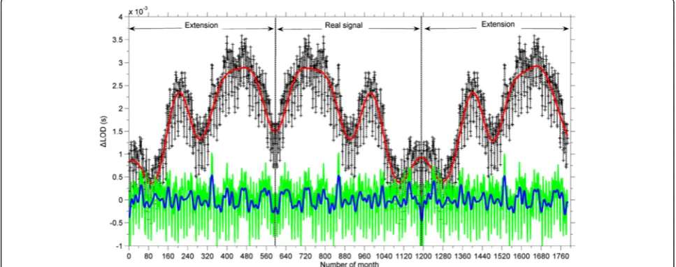
Wavelet transform owns the edge effect (Zheng et al. 2000), which can bring some errors into the final results. In order to study the 6-year signal using NMWT method quantitatively, we need to eliminate the edge effect. The commonly effective method of eliminating the edge effect is to make a symmetrical extension at the two boundaries of LOD data (see Fig. 1). We can get the interannual variations (see the blue curve in Fig. 1) after filtering the seasonal signals from the residual series, where the residual series referring to the decade has been removed from the original series. The red curve is the decade term; the green curve is the residual of dec-ade subtracted from original LOD; and the blue curve is interannual variations that seasonal and decade terms
have been removed. “Real signal” means the original LOD series from 1962 to 2012;“Extension” refers to the symmetric extension parts. But we have to test whether the target interannual signal is disturbed or not during the above filtering process. Consequently, we make a further detailed comparison of the signal before and after filtering (see Fig. 2). Figure 2 shows that the fre-quency spectrum of the above two signals is in exact agreement with each other within the frequency scope 0.0083 cpm <f< 0.051 cpm.
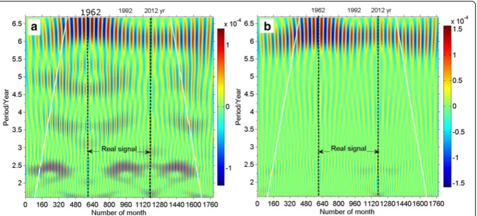
Numerous publications show that AAM (motion term + mass term) is a primary contributor to interan-nual variations in LOD (Abarco del Rio et al. 2000, 2003; Holme and de viron 2013; Chen 2005; Chao and Yan 2010). Consequently, we should remove the AAM effect from the original LOD series. Figure 3a shows that we can divide the spectrum of original LOD series into two frequency bands, i.e., 1.6–5 years and 5– 6.7 years. Comparing Fig. 3a with Fig. 3b, we can see that, after the AAM was removed, the signals in 1.6~5-year band are greatly weakened while the 5~6.7-1.6~5-year signals are almost uninjured but the 6-year signal show-ing more notable.
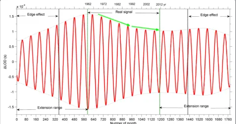
To further investigate the harmonic feature of the 6-year signal, we take the modulus of Wgf(a,b) (NMWT spectrum), i.e., |Wgf(a,b)| (see Fig. 4). Where Wgf(a,b) means applying NMWT to time signalf(t) (i.e., the LOD time series on the interannual scales);gsignifies the nor-mal Morlet wavelet; and a and b are scale factor and translating index, respectively. From Fig. 4, we can see the continuous and stable “ridgeline” (the thin black lines are the local maxima, and they represent the in-stantaneous frequency or periodic variations) for the corresponding quasi-harmonics in |Wgf(a,b)| spectrum on 1.6–6.7-year scales. Consequently, it is valid to see the 6-year signal as a quasi-harmonic signal according to the viewpoint from Liu et al. (2007) that NMWT values along the “ridgeline” recovering the corresponding quasi-harmonics. Figures 5 and 6 are respectively the corresponding 6-year quasi-harmonics signals from ori-ginal series and the AAM removed series, which are
Fig. 2Comparison of the signals before and after filtering the seasonal signal from LOD original series in which decadal variations were removed. This figure shows that we have to study the interannual variations within 0.0083 <f< 0.051 cpm (i.e., periodic range: 1.6 years <T< 10 years)
Fig. 4Comparison of the |Wgf(a,b)| spectrum fromaoriginal LOD series andbthe AAM effect (motion term + mass term) has been removed, on 1.6–6.7-year scales. Theblack linesrefer to“ridgeline”, and the location of“ridgeline”shows the instantaneous periodic of the target signals. We can recover the target 6-year signal through extracting the wavelet transform coefficient real part values that the“ridgeline”corresponds to, from the NMWT spectrum, without inverse transformation, directly and quantitatively
both extracted by NMWT. Obviously, the target 6-year signal (i.e., the real signals present in Figs. 5 and 6) shows the decreasing trend in the whole, which is unre-lated to the wavelet edge effect.
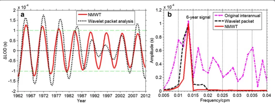
In order to ensure the accuracy of the target signal extracted by NMWT and verify the superiority of NMWT method in extracting signals, we extract the tar-get signal using two methods respectively and then make a detail comparison of the above two results in both time and frequency domains. The first method is using wavelet packet method based on the orthogonal Daubechies let with higher-order vanishing moment; where the wave-let packet method can provide a fine analysis of the signal (the detailed principle of wavelet packet analysis will not be repeated again in this paper). According to the principle of wavelet packet analysis and the sampling rate of LOD data (30 days) in this paper, we can obtain the sig-nals in a 64~96-month band (i.e., 5.3~8 years) (see Fig. 7a). Here, the order of (Daubechies wavelet) vanishing moment (N) is 45 and the corresponding compactly sup-ported length is 89. Choosing the higher order of vanish-ing moment can help us extract signals with more accuracy (Daubechies 1988; Hu et al. 2005, 2006). The second method is using NMWT method; we extract the instantaneous values that the “ridgeline” corresponds to, from NMWT spectrum (Liu et al. 2007); thus, we can get the target signal with accurate phase in the time domain, whose frequency spectrum peak is very close to 0.0138 cpm (see Fig. 7a, b).
Figure 7a indicates that the signal from wavelet packet method shows an obvious decreasing phenomenon in the 1990s, which is consistent with a previous study (Abarco del Rio et al. 2000; Holme and de viron 2013; Gorshkov 2010); however, Fig. 7a also shows the signal based on NMWT is gradually weakening during 1962– 2012 instead of abrupt change in some period. Figure 7b reveals the three Fourier amplitude spectrum peaks (all values are about 0.104 ms) locating at 0.0138 cpm, from original signal and wavelet packet and NMWT, are very consistent with each other; but, obviously, the signal with the most concentrated energy and the most narrow frequency range and no side-lobe interference and the very ideal filtering effect is from NMWT method.
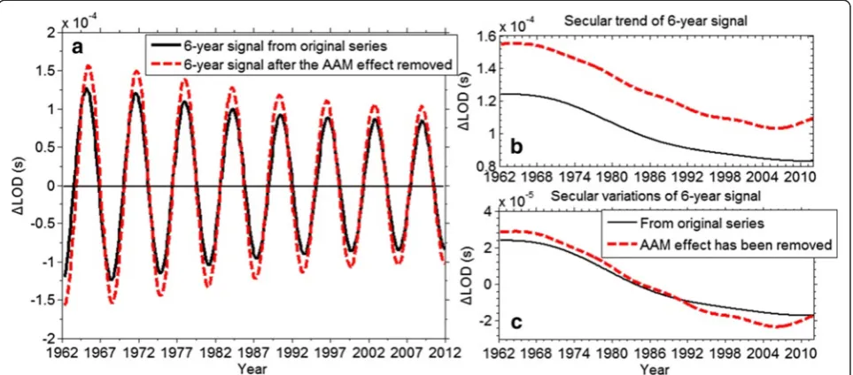
Figure 8a shows the variation feature of the 6-year signal in which AAM effect has been removed. The long-term reduction is about 0.5 × 10⁻⁴s (0.05 ms) dur-ing 1962~2012 years. The ratio of the above reduction (0.05 ms) to the mean amplitude of (0.124 ms) reaches about 40 %. Figure 8b indicates that the magnitude of the 6-year signal with a mean amplitude of 0.124 ms concentrates closely at the 0.0138 cpm, which demon-strates the 6-year signal based on NMWT method should be reliable and correct. Talking about the above, the concept about long-term variation of the 6-year signal extracted by NMWT method can be de-fined as follows: the total envelope curve variation trend of the 6-year signal is called the long-term vari-ation of this signal.
Making a further comparison of the 6-year signal be-fore and after the AAM effects were removed, we can see clearly the contribution from AAM effect to the 6-year signal (Figs. 9a, b). An obvious conclusion that can be made is that AAM always cancels out the strength of the 6-year signal, which also shows that the contribution from AAM to the 6-year signal is about 0.026 ms, which occupies the mean amplitude of 0.124 ms about 21 %. Figure 9c suggests that the long-term trend change of the 6-year signal is very consistent with that of the AAM removed, which means the above long-term decreasing phenomenon is unrelated to the AAM effect. Conse-quently, there should be other uncertain components causing the decreasing phenomenon.
In order to display the results of this paper clearly, we have plotted Fig. 10 with the result from Fig. 6 and the
background trend series that has been removed by wave-let filtering.
Discussion
In this study, we find the 6-year signal in LOD showing the long-term decreasing trend during the past 50 years, which is unrelated to AAM effects. We have a careful review about the result of this paper. In order to test the reliability of the result from NMWT and further verify whether the instantaneous amplitude of the 6-year signal is constant or varying with time, a simple and effective method is used, which is windowed Fourier transform.
We need to compare the relative amplitude values of applying windowed Fourier transform to LOD series (AAM effect has been removed) in different periods. The detailed data preprocessing method is as follows:
Fig. 8The 6-year signal of LOD in which AAM effect has been removed, in the time domain (a) and its Fourier spectrum, in the frequency domain (b). From Fig. 8, we can see the long-term amplitude decreasing trend
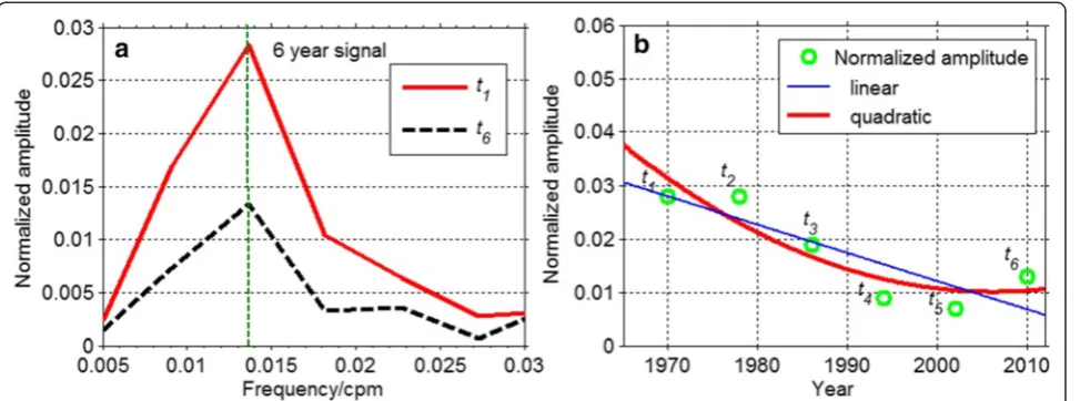
firstly, applying 1-year running average to eliminate the seasonal variations in the LOD series (1962~2012); sec-ondly, fitting the decadal term using 10-order polynomial and remove it from LOD series. We divide the time span (i.e., 1962~2012) into six periods, which are respective t1 (1962~1980), t2 (1968~1986), t3 (1974~1992), t4 (1980~1998), t5 (1986~2004), t6 (1992~2010); and then, we compute the normalized Fourier amplitude spectrum one by one in ti (i= 1,2,…6) period and obtain all the spectrum peak values locating at about 0.0138 cpm in each frequency domains (see Fig. 11). Figure 11a shows the comparison of relative amplitude values in t1and t6 periods. From Fig. 11a, we also can see that the relative amplitude of the 6-year signal int1period is about 0.0275, which is larger than that (about 0.0135) int6. The ratio of the former to the latter is about 2, while the result from NMWT gives the ratio about 1.5 (see Fig. 8a). Because we cannot guarantee that 3 cycles of the 6-year signal can exactly and completely locate each chosen period (i.e.,ti), some errors in the above method are possible. How-ever, the 6-year signal strength decreasing from t1 to
t6 period is beyond doubt. Figure 11b further shows all the relative amplitude values of the 6-year signal in the above six periods and, overall, the spectrum peaks is showing the declining trend, which is con-sistent with the result of NMWT.
On the other hand, in theory, if the 6-year signal is a stable harmonic signal with an invariant amplitude, it will be recovered precisely by NMWT method with a constant amplitude, which is determined by the proper-ties of NMWT (Liu et al. 2007). Moreover, the long-term reduction is so large that it has occupied the mean
amplitude (0.124 ms) about 40 %, which means the above phenomenon cannot be simply attributed to the errors produced in data processing or the method this paper uses. However, the result based on the wavelet packet gives us some enlightenment to resolve the debates on the variation feature of the 6-year signal in LOD from previous studies. We propose a viewpoint that the 5~8-year signal from wavelet packet shows a decreasing phenomenon in the 1990s (Fig. 7a), which may be the result of the 6-year signals beating against
Fig. 9Comparison of the 6-year signal from original series and that after the AAM was removed (a); Comparison of the variations of envelope curves (b, c). Theblack curveis the original 6-year variations;red curveis AAM effect removed. Figure 9 also shows the contribution from AAM effects to the 6-year signal. The AAM effect always reduces the strength of the 6-year signal
the other frequency signals in the 5~8-year bands (see Figs. 8b and 7b).
Then, what is the geophysical mechanism of causing the long-term decreasing of the 6-year signal? Many pa-pers (Abarco del Rio et al. 2000, 2003; Chen 2005; Chao and Yan 2010) showed that ΔLOD (i.e., the variation of LOD) consists of two terms: motion term and mass term; where motion term contains zonal wind and ocean current excitation; as to the zonal wind excitation, we have removed it from LOD in the AAM. Previous stud-ies (Marcus and Chao 1998) demonstrated that ocean has a low contribution to seasonal variations in LOD (less than 5 %); its contributions on interannual or lon-ger scales can also be negligible (Abarco del Rio et al.
2000). Thus, we exclude the ocean excitation. Our sup-position is that it is mainly related to the mass term of
ΔLOD. The mass term is determined by the mass redis-tribution and total mass change within the Earth system. The mass term can be expressed as (Chao and William 1988; Bourda 2008):
ΔLODð Þ ¼t 2 3
MR2 e Cm Δ
J2ð Þ þt 1þk′2 ΔM
M
LODmean
ð9Þ
whereM is the Earth’s mass of about 5.98 × 1024kg;Cm
is the principal moment of inertia of the Earth’s mantle
of about 7.1 × 1037kgm2;Reis the Earth’s mean radius of Fig. 11Comparison of the relative amplitudes of the 6-year signals int1andt6periods (a); the total variation trend of the amplitudes in six periods in time domain and thegreen cyclesrefer to the relative amplitudes of the 6-year signal in various periods (b); the time window this paper uses is hamming window
about 6,372,797 m; ΔJ2 expresses the change of Earth’s dynamic oblateness, which is related to the Earth’s
prin-cipal moment of inertia (Cheng et al. 2013; Cheng and
Tapley 2004; Cox and Chao 2002; Dickey et al. 2002);
ΔM signifies the Earth’s total mass change, which is
in-dependent of the mass geographical distribution (Chao
and William 1988; Yan and Chao 2012); k′2 is the love
number of−0.31; and LODmean= 86400 s. The ΔJ2data
is from Cheng et al.(2013) based on Satellite Laser
Ranging (SLR) at 30-day intervals from 1976–2011.
Figure 12a indicates that the secular variation of ΔJ2is showing a quadratic decreasing trend, but not the linear trend (Cheng et al.2013).
Formula (9) contains the following two possibilities: The first possibility ΔM≡0, namely the total mass is conserved within the Earth system; then, formula (9) shows the mathematical relationship between ΔJ2 and
ΔLOD. We can compute the“equivalent” mass-induced
ΔLOD, because the long-term variation is mainly related to the PGR-poster glacial rebound and melting of the glaciers and ice-sheets mass change (Cheng et al. 2013). Consequently, under the condition of mass conservation,
ΔLOD is also determined by the same above factors. Figure 12b shows that the contribution from mass redistribution within the Earth system is consistent with long-term change of the 6-year signal in trend, but the former decreasing rate is about three times larger than that of the latter. Consequently, there should be other components to prevent the long-term decreasing rate of the 6-year signal.
The second possibilities: ΔM≠0, namely, considering of the GMB effect (Yan and Chao 2012). Assuming that the secular decreasing trend of the 6-year signal can be fully interpreted by formula (9), thus, we can get ΔM
within the Earth’s system, in turn. By calculation, the secular ΔM change is in a mean rate of about +2.1 × 10¹⁴kg/year, from 1976~2011, however, the actual secu-lar variation ofΔM, especially its precise value, is still to be further studied due to its some unknown factors, while the results from Yan and Chao (2012) indicated that the annual amplitude of ΔM caused by Earth’s
sur-face geophysical fluids including atmospheric, oceanic, and land hydrology (i.e., GMB effect) reaches about 41.7 × 10¹⁴ kg. Basing from above, the global total mass change ΔM reaches about +7.63 × 10¹⁵ kg, during 1976~2012. Given that a mean sea level of 1 cm corre-sponds to a ΔM of 3.6 × 10¹⁵ kg (Chao and William 1988), the sea level has risen by 2.1 cm during the past 36 years. It is essential to estimate accurately the GMB long-term effect for interpreting the secular decreasing phenomena of the 6-year signal.
Then, will the secular decreasing trend of the 6-year signal come from the Earth’s core? This is required to be further explored.
Conclusions
This paper extracts the 6-year temporal signal without AAM effects using NMWT method, quantitatively. The 6-year signal from NMWT shows the following features: 1) the signal with accurate phase, that is, the phase shift-ing does not happen; 2) the signal with a very narrow frequency range and a high energy concentration degree and a mean amplitude of about 0.124 ms; 3) the secular trend showing a continuous decreasing trend during the past 50 years instead of the abrupt change in some periods. Two possibilities in explaining the long-term decreasing of the 6-year signal are given. We hope this paper can provide a valuable reference for investigating the 6-year signal quantitatively and resolving its geo-physical mechanism ultimately.
Competing interests
The authors declare that they have no competing interests.
Authors’contributions
PD and GL proposed the topic and the analysis method and also performed analysis; LL, XHu, XHao, and YH collaborated with PD and GL in discussing the analysis method and LL further checked the correctness of the analysis method that this manuscript uses. ZZ and BW carried out the data selection and quality control. All the authors read and approved the final version of the manuscript.
Acknowledgements
The authors acknowledge the Institute of Geodesy and Geophysics, CAS, for providing computational resources. This work is supported by National Natural Science Foundation of China (grant 41321063, 41374029) and the State Key Laboratory of Geodesy and Earth’s Dynamics Foundation (grant SKLGED 2013-4-1-Z).
Author details
1
Institute of Geodesy and Geophysics, Chinese Academy of Sciences, State Key Laboratory of Geodesy and Earth’s Dynamics, Wuhan 430077, China.
2
University of Chinese Academy of Sciences, Beijing 100049, China.
3Department of Physics, School of Science, Wuhan University of Technology,
Wuhan 430070, China.
Received: 13 June 2015 Accepted: 14 September 2015
References
Abarco del Rio R, Gambis D, Salstein DA (2000) Interannual signals in length of day and atmospheric angular momentum. Ann Geophys 18:347–364 Abarco del Rio R, Gambis D, Salstein D, Nelson P, Dai A (2003) Solar activity and
earth rotation variability. J Geodyn 36:423–443
Bourda G (2008) Length-of-day and space-geodetic determination of the Earth’s variable gravity field. J Geod 82:295–305
Chao BF (1989) Length-of-day variations caused by EI Nino-southern oscillation and quasi-biennial oscillation. Science 243:923–925
Chao BF, William PO (1988) Effect of uniform sea-level change on the Earth’s rotation and gravitational field. Geophys J 93:191–193
Chao BF, Yan HM (2010) Relation between length-of-day variation and angular momentum of geophysical fluids. J Geophys Res 115:B10417. doi:10.1029/ 2009JB007024
Chao BF, Chung WY, Zong R, Shih, Hsieh YK (2014) Earth’s rotation variations: a wavelet analysis. Terra Nova 26:260–264
Chen JL (2005) Global mass balance and length-of-day variation. J Geophys Res 110:B08404. doi:10.1029/2004JB003474
Cheng MK, Tapley BD (2004) Variations in the Earth’s oblateness during the past 28 years. J Geophys Res 109:B09402. doi:10.1029/2004JB003028
Cox CM, Chao BF (2002) Detection of a large-scale mass redistribution in the terrestrial system since 1998. Science 297:831–833
Daubechies I (1988) Orthonormal bases of compactly supported wavelet. Commun Pure Appl Math 41:909–996
Davies CJ, Stegman DR, Dumberry M (2014) The strength of gravitational core-mantle coupling. Geophys Res Lett 41, doi:10.1002/2004GL059836 Dickey JO, Marcus SL, Viron O, Fukumori I (2002) Recent Earth oblateness
variations: unraveling climate and postglacial rebound effects. Science 298:1975–1977
Gorshkov VL (2010) Study of the interannual variations of the Earth’s rotation. Sol Syst Res 44:487–497
Holme R, de Viron O (2005) Geomagnetic jerks and a high-resolution length-of-day profile for core studies. Geophys J Int 160:435–439
Holme R, de Viron O (2013) Characterization and implications of intradecadal variations in length of day. Nature 499:202–205
Hu XG, Liu LT, Hinderer J, Sun HP (2005) Wavelet filter analysis of local atmospheric pressure effects on gravity variations. J Geod 79:447–459 Hu XG, Liu LT, Hinderer J, Sun HP (2006) Wavelet filter analysis of atmospheric
pressure effects in the long-period seismic mode band. Phys Earth Planet Inter 154:70–84
Liu LT, Hsu HT, Grafarend EW (2007) Normal Morlet wavelet transform and its application to the Earth’s polar motion. J Geophys Res 112:B08401. doi:10.1029/2006JB004895
Mandea M, Holme R, Pais A, Pinheiro K, Jackson A, Verbanac G (2010) Geomagnetic jerks: rapid core field variations and core dynamics. Space Sci Rev 155:147–175
Marcus SL, Chao Y (1998) Detection and modeling of nontidal oceanic effects on Earth’s rotation rate. Science 281:1656–1659
Mound JE, Buffett BA (2003) Interannual oscillations in length of day: implications for the structure of the mantle and core. J Geophys Res 108(B7):2334. doi:10.1029/2002JB002054
Mound JE, Buffett BA (2006) Detection of a gravitational oscillation in length-of-day. Earth Planet Sci Lett 243:383–389. doi:10.1016/j. epsl.2006.01.043
Silva L, Jackson L, Mound J (2012) Assessing the importance and expression of the 6 year geomagnetic oscillation. J Geophys Res 117:B10101. doi:10.1029/ 2012JB009405
Wang QL, Chen YT, Cui DX, Wang WP, Liang WF (2000) Decadal correlation between crustal deformation and variation in length of day of the Earth. Earth Planets Space 52:989–992
Yan HM, Chao BF (2012) Effect of global mass conservation among geophysical fluids on the seasonal length of day variation. J Geophys Res 117:B02401. doi:10.1029/2011JB008788
Zheng D, Chao BF, Zhou Y, Yu N (2000) Improvement of the edge effect of the wavelet time-frequency spectrum: application to the length-of-day series. J Geod 74:249–254
Submit your manuscript to a
journal and benefi t from:
7 Convenient online submission
7 Rigorous peer review
7 Immediate publication on acceptance
7 Open access: articles freely available online
7 High visibility within the fi eld
7 Retaining the copyright to your article