R E S E A R C H
Open Access
Detection, 3-D positioning, and sizing of small
pore defects using digital radiography and
tracking
Erik Lindgren
Abstract
This article presents an algorithm that handles the detection, positioning, and sizing of submillimeter-sized pores in welds using radiographic inspection and tracking. The possibility to detect, position, and size pores which have a low contrast-to-noise ratio increases the value of the nondestructive evaluation of welds by facilitating fatigue life predictions with lower uncertainty. In this article, a multiple hypothesis tracker with an extended Kalman filter is used to track an unknown number of pore indications in a sequence of radiographs as an object is rotated. Each pore is not required to be detected in all radiographs. In addition, in the tracking step, three-dimensional (3-D) positions of pore defects are calculated. To optimize, set up, and pre-evaluate the algorithm, the article explores a design of
experimental approach in combination with synthetic radiographs of titanium laser welds containing pore defects. The pre-evaluation on synthetic radiographs at industrially reasonable contrast-to-noise ratios indicate less than 1% false detection rates at high detection rates and less than 0.1 mm of positioning errors for more than 90% of the pores. A comparison between experimental results of the presented algorithm and a computerized tomography reference measurement shows qualitatively good agreement in the 3-D positions of approximately 0.1-mm diameter pores in 5-mm-thick Ti-6242.
Keywords: Radiography; Nondestructive evaluation; Chain porosities; Laser welding; Image analysis; Multiple hypothesis tracker
1 Introduction
Radiographic inspection is frequently used within the manufacturing industry to detect and characterize defects in a wide variety of structures. The characterization gen-erally consists of determining the defect type, size, and position within the structure. The size together with its distance to other defects and to the surface are known to affect the fatigue life of the structure [1]. This results in three issues: firstly, the size is of interest to measure in itself; secondly, the size is also of interest since assum-ing no interaction between the defects, the smallest defect that can be detected with high probability, will be a param-eter limiting the predicted fatigue life; and thirdly, the distance which is of interest is in three-dimensional (3-D). However, only the distance in two-dimensional (2-D) is
Correspondence: [email protected]
Department of Materials and Manufacturing Technology, Chalmers University of Technology, Gothenburg SE-412 96, Sweden
available from conventional projection radiography, and the distance in the third dimension therefore has to be assumed. These three issues are encountered, for example, with components built by laser-welded thin lightweight alloys. Lightweight titanium alloys are extensively used within the aero industry, and laser welding of these alloys are increasing. However, the combination of lightweight alloys and laser welding, including welding methods sim-ilar to it, has been shown to result in the formation of clusters of small submillimeter pores in the melted zone of the weld [2,3]. The pores are small (the average diam-eter is 0.4 mm), and as isolated defects, their effect on fatigue life is considered negligible. However, if they can-not be considered as isolated defects, depending on their size, they might no longer be negligible. Therefore, there is a need to detect small, low contrast-to-noise ratio (CNR) defects and to measure their size and 3-D positions.
The 3-D positioning has been solved by two funda-mentally different approaches in the literature. The first
approach is based on reconstructing the whole bulk vol-ume using computerized tomography (CT). However, a complete set of projections over the whole 180° rota-tion is needed, and some structures, for example planar structures, are therefore difficult to reconstruct. In certain situations, the problem with an incomplete rotation set can be solved by means of limited view tomography [4]. The second approach is based on not reconstructing the whole volume but rather by focusing on reconstructing the 3-D position of each defect, referred to as point recon-struction methods [5]. In point reconrecon-struction, the 3-D position of the defect is calculated using the defect pro-jection coordinates in the image plane for a few rotations and/or translations.
The problem of detecting low CNR defects and of mea-suring their size has instead received attention within the more general automatic weld inspection analysis field. The automatic analysis field approach is in general to seg-ment out any possible defect [6] and then characterize it [7-9], for example, by its type (lack of fusion or crack etc). A merge between the segmentation part of the general automatic analysis and the 3-D point reconstruction has been shown to result in a high probability of detecting true defects and a low probability of detecting false defects, especially for low CNR defects [10]. After segmenting out the defect indications in the detector plane, there will be more false defects than true defects detected due to low CNR. The true defects will form paths in the detector plane as the object is rotated or translated, while the false defects will not. The performance has been improved by adding the classification step and removing the need for prior knowledge of the setup geometry in [11]. If the 3-D positions of the defects are not needed, they can instead be used implicitly as in [12] where the defects are tracked during constant translation to yield a computationally less expensive algorithm.
The currently presented solutions to the coupled low CNR and 3-D point reconstruction problem all have in common that the defect needs to be detected in all rota-tion projecrota-tions. This need is difficult to fulfill as the defect CNR decreases. Furthermore, the defect can also fail to be detected in some rotation projection due to extreme X-ray interactions. These extreme interactions will eventually occur, though with low probability, due to the inherent statistical nature of radiographic inspection. However, this need of full detection is removed in the solution proposed here. Instead of being formulated as a vision system problem and solved by epipolar geometry as in [10,11], it is explored using general tracking the-ory [13]. In tracking thethe-ory, the state (3-D position) of an object (defect) is tracked by assigning measurements (indications) to it as time increases (rotation). In general, the measurements do not have to be present in all time points for the object to be successfully tracked. Therefore,
a tracking theory approach will take advantage of the path of defect indications in the detector plane without mak-ing it a limitation by demandmak-ing the defect to be detected in all rotations. The main value of this work is that it con-siders the coupled low CNR and 3-D point reconstruction problem from a general tracking theory point of view.
The defect size is measured by considering the change in intensity over the defect indication compared to the background together with an intensity calibration, a pro-cedure considered conventional in radiography. However, a systematic methodology to set up optimal parameters for the algorithms, including this last one, is proposed. The methodology consists of using design of experiment (DOE), robust design, and synthetic radiographs.
The outline of this article is as follows. First, the radio-graphic inspection procedure together with the algorithm is described. This is followed by an explanation of how simulated radiographs are used to set up the algorithm and to evaluate its performance. The result of the perfor-mance evaluation using the synthetic radiographs is then presented. This is followed by a description of the experi-mental setup and the experiexperi-mental qualitative results.
2 Algorithm and inspection procedure
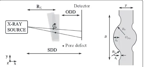
The radiographic inspection setup geometry and the pro-cedure is illustrated in Figure 1. Common setup geometry parameters such as source to rotation pointxcoordinate (Rx), source to detector distance (SDD), and object to detector distance (ODD) are defined in the figure. The intended inspection application is to detect, position, and size submillimeter pore defects in thin (≈ 5 mm) laser-welded titanium. The laser weld geometry parametriza-tion [14] is also indicated in Figure 1. The parameters are nominal thickness(T), weld width (B), enforcement radius(R0) and thickness(δ0), and undercut radius(R1) and thickness(δ1).
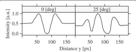
The image analysis of the radiographs faces two main difficulties, which are illustrated with synthetic radio-graphs. Firstly, as can be seen in Figure 2, large-scale vari-ations over small pixel length scales in the projected weld
Distance y [px] Intensity [a.u.] 0.0
0.5 1.0
50 100 150 0 [deg]
50 100 150 25 [deg]
Figure 2Weld geometry line profiles.Two line profiles at 0◦and 25◦rotation taken from simulated radiographs perpendicular to the welding direction. Both profiles are arbitrarily scaled and offset for illustrative purposes.
geometry dominate the gray scale variation compared to the pore indications shown in Figure 3. The pore indica-tions in Figure 3 are some 20 to 30 times smaller than the large-scale variations in Figure 2. Secondly, as indicated in Figure 3, the CNR of the pore indications are low. For pores at the size of the detector pixel size, the contrast is highly sensitive to the pore size. The contrast is approx-imately proportional to radius3or even worse depending on its size compared to the detector pixel size. Further-more, the pore indication is small in terms of affected number of detector pixels.
The algorithm is divided into the following three tasks: segmentation, tracking, and size measurement. The seg-mentation output is a set of coordinates of pore projection indications in the radiographs from the different rota-tions. This list is input to the tracker, which solves for the 3-D coordinates at the same time as it filters out false pores. The pores proposed as true pores are then paired up with their projection coordinates and used as input to the size measurement algorithm. It should be noted that the concept is to retrieve what is interesting, the
Distance z [px]
Intensity [a.u.
]
0 1
0 100 200 300 400 500 600 700 800
0 1
Figure 3Pore indication line profiles.Line profiles from simulated radiographs representing the low and highcnr. In total eight pores
are indicated by dotted lines at radii(0.055, 0.065. . .0.125 mm). The intensity is approximately 20 to 30 times less than the the intensity in Figure 2.
pore indications, rather than to first make a low-noise radiograph.
2.1 Segmentation
The segmentation should output a set of 2-D pixel coor-dinates representing the mass centers of all pore indica-tions in each of the radiographs. It is preferred to have a high true-positive rate, a low false-positive rate, a high precision in the mass centers, and a high uniqueness. Where a high uniqueness is defined as each pore coor-dinates is only listed once among the coorcoor-dinates, three different segmentation methods (see Figure 4) have been evaluated: a radial symmetry based, a cross correlation, and an energy weighted cross correlation. To address the uniqueness, a merger algorithm common to all methods is applied as a final step.
2.1.1 Radial symmetry
The idealized pore will be projected with circular symme-try in the intensity pixel values around the mass center point when the intensity is otherwise constant. Therefore, a high level of circular symmetry is expected to be a good measure of a pore projection center. In [15], a measure of local symmetry based on normalized axial moments is derived and implemented as a discrete symmetry trans-form (DST). The DST is calculated as given in [15,16] according to
DST(i,j)=1−
k(Tk(i,j)2)
nrs −
kTk(i,j)
nrs 2
,
(1)
Tk(i,j)= 1 Tmax
(l,m)Cr
|(i−l)sin(kπ nrs
) (2)
−(j−m)cos(kπ nrs
)|lrs×I(l,m).
The sum in Tk(i,j) is summed over the indexes which are on the boundary of the pixelated circleCr of radius rrs with pixels centered in(i,j). In total, nrs number of local axial momentsTkat the orderlrsare calculated and summed over withk=0,. . .,nrs−1 at eachi,j. The max-imum value ofTkis then used as the normalization factor
Tmax. The transform will look for symmetry around the axis with slope given bykπ/nrs, that is, axes in the case of nrs>1.
In [15], the DST is only applied at points of nonunifor-mity; here, the nonuniformity stage is changed to identify potential pore projection center points instead. The fol-lowing differential expression is proposed to identify a symmetric peak around the second indexjwith possible radius≈rrs:
E(i,j)=[I(i,j+rrs)−I(i,j+rrs+1)]
+[I(i,j−rrs)−I(i,j−rrs−1)] , (3)
where the direction of index j is perpendicular to the weld geometry. Ewill be large when slopes are opposite around(i,j)and, for example, identical to zero for a per-fect line. As a final step, the DST matrix is convoluted with a Gaussian kernelGwith standard deviationσrsresulting in a correlation image:
Crs(i,j)=(E(i,j)×DST(i,j)) G. (4)
This procedure is runirsnumber of times for differentrrs, with the result averaged. It should be noted that when the number of axial moments is set to 1 (nrs=1), the correla-tion image will only depend onE(i,j)since DST(i,j) = 1 for alli,j.
2.1.2 Cross correlation
If a mathematical model of the pore projection can be derived, such a model can be correlated against the image to find correlation maximums and hence the locations of the pore indications. The same linear X-ray attenuation model as in [14] is used but with the detector approxi-mated as ideal and the X-rays approxiapproxi-mated as parallel. The 2-D projection of the pore with radius rcc pixels centered incis approximated as
K(i,j)∼e2μ√r2cc−[(i−c)2+(j−c)2]−1, (5)
where μ is the linear attenuation per pixel for the sur-rounding material. Furthermore, the equation is only valid for(i−c)2+(j−c)2≤r2
cc.
The detector model used for the synthetic radiographs will smooth the pore projection indications due to its point spread function. This smoothing will also be present in real radiographs. However, due to the idealized detec-tor model used, this effect is not included in Equation 5. Furthermore, the buildup factor (fraction of scattered to direct radiation) is assumed to be approximately constant over the area of the projected pore. This has been shown to hold for this application in [14]. Finally, probably the least valid assumption is that the background intensity profile, in this case dominated by the weld geometry, is changing little compared to the change due to the pore.
This assumption is not valid, and therefore, geometry-related intensity changes must be reduced. This reduction is done using a simple local median with radius rme, I(i,j)=I(i,j)−Median
k,lrmeI(i±k,j±l). As a last step,
the normalized cross correlation is calculated at each pixel against the model proposed in Equation 5 according to the standard equation:
Ccc(i,j)= (6)
(l,m)K(l,m)×I(i+l,j+m)
(l,m)(K(l,m)− K)2×I(i+l,j+m)2
,
where the summation is over all indexes within a square of sizesccanddenote average. A value close to 1 will indicate a high similarity toK.
A variation of the cross correlation method is also con-sidered and referred to as energy weighted cross correla-tion. The cross correlation is scaled with the energy in the intensity according to
Cene(i,j)=Ccc(i,j)×
(l,m)
I(i+l,j+m)2, (7)
where the indexesl,mis given byK(l,m) =0.
2.1.3 Mean shift merging
The last step of the segmentation is a merger algorithm, which intends to make the coordinates unique. The algo-rithm is based on the mean shift algoalgo-rithm [17]. The mean shift algorithm is generally used to find high-density regions (clusters) in multidimensional spaces. Here, it is used to find the centers of pore indication clusters in 2-D. In more detail, the merger iteratively selects the pixels in the correlation image with values larger thanCT. For each pixel aboveCT, the mean shift algorithm is restarted and iterated until it has converged into a local maximum in density. At each iteration, the mass center within a radiusrms is calculated and compared with the previous mass center, the mean shift vector. In the next iteration, this next proposed mass center is used. This is repeated until the solution is considered as having converged, with the mean shift vector changing less thanδmspercent. The converged coordinates are incrementally averaged in bins of 1-pixel sizes. As a consequence, indications closer than ≈rmswill not be resolvable.
2.2 Tracking
object is updated when a new measurement is assigned to it (filtering). The measurements are the set of pore projection coordinates in the detector plane given by the segmentation.
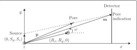
The filtering step consists of measurement prediction and object state vector update. It is often handled by a member of the Kalman filter family (see for example [18]). In this article, the extended Kalman filter (EKF) is used since the measurement functionY = h(X)is nonlinear. The nonlinearity is rather low, and the EKF is assumed to be sufficient. The filter state variables are the 3-D coordi-natesp=(px,py,pz)of each of the pores and the rotation angleω. The mass center coordinatesmof the projection of an ideal pore following the notations in Figure 5 are given by
my=
SDD[Txsinω+Tycosω+Ry−Sy] Txcosω−Tysinω+Rx +
Sy,
mz=
SDD[pz−Sz] Txcosω−Tysinω+Rx +
Sz, (8)
Tx=px−Rx, Ty=py−Ry,
where m is in millimeters and is translated and scaled into the detector plane before it is used. These equations are then linearized in the EKF framework, and a stan-dard Kalman filter approach is applied. The measurement errors are assumed to be Gaussian with a diagonal covari-ance matrix. The diagonal elements are denoted R for the pore indication coordinates andRωfor the angle. The states will typically oscillate weakly, an effect which can be modeled by a nonzero state covariance matrix. How-ever, it is set to zero since the oscillations are assumed to be negligible compared to the measurement errors. Being linearized, the EKF is sensitive to the initial state. However, in some cases an initial state close to the true state can be derived from two measurements; therefore, the state initiation is delayed until measurements from two rotations are present. Allowing rotation only around one of the euclidean base vectors, one can solve the two
Figure 5Setup geometry.The pore mass center with position vectorpis rotated with an angleωaround thez-axis with respect to the rotation point(Rx,Ry, 0). The pore is projected on the detector plane atm=(SDD,my,mz)(see also Figure 1).
equations in Equation 8 for the two unknown coordi-nates (px,py). Additionally, pz is approximately known from the rotation axis limitations. The state initiation is accepted if Gx0 < px < Gx1 and otherwise rejected. The gatesGx0andGx1are approximated from the setup geometry. The initial state could also be derived using the formalism of vision systems, relaxing the demand on rotation axis, though this approach has not been taken here.
One data association method suitable for the situation is the multiple hypothesis tracker (MHT) originally pre-sented in [19]. It is suitable when the number of objects to track is not known a priori and/or when the clutter density is high. The implementation derived is very sim-ilar to the ‘Structured Branching’ MHT as described in [20]. The assumptions made are that each object gener-ates at most one measurement but each measurement can originate from many different objects. The last assump-tion accepts overlapping pore projecassump-tions in some of the rotations.
In the nomenclature of tracking, as the object changes its state in some partly known way, the measurements belonging to it forms a track and the track can be used to solve for the state. The main idea of the MHT is that it computes many possible tracks from different combina-tions of measurements and selects only the most probable. The different combinations can be kept in a tree, with the path from each leaf to the root representing one solution. The probability for each track (object) to be a true positive is, if it is not properly normalized, referred to as its score. The score is constructed by the summation over all nodes, one at each rotationk, for each track as log likelihoods according to
scorek=scorek−1+ score, (9)
score= −d02, (10)
score=Smht×ln
1/ det(RS)
−d2, (11)
where Equation 10 refers to the case of no measurement (the pore indication is not detected in the radiograph) and Equation 11 refers to when a measurement is present. RS is the measurement residual covariance matrix, which increases withR,Rω, and the covariance matrix calculated in the Kalman filter step.Smht is a scaling parameter to weight the two terms. Further,d2is a normalized statisti-cal distance indicating how far away the measurement is from the prediction with respect to the uncertainty indi-cated by RS. See [13] for an in-depth discussion on the constants and the scores.
1 for each rotation 2 for each root 3 for each leaf
4 for each measurement
5 gate
6 add node
7 add no measurement node 8 for each leaf
9 prune
10 add roots 11 decide 12 combine
Adding new nodes to the tree is done with great care for the tree not to grow too large. The gates Gz andGy are applied on the two detector coordinates (row 5). If the dif-ference between the previous measurement and the new one is within the gates, a new node for the measurement is added (row 6). There is always a node added for the no measurement case (row 7). The no measurement case represents the hypothesis that the measurement was not detected in the current rotation.
Apart from the gating, a pruning of the tree is also con-ducted. At the pruning (row 9), the leaves withscore = scorek/k ≥ T1 are accepted and kept while the rest are rejected and pruned. In addition, a maximum limit of five leaves per root is applied, where the leaves with the highest score are kept. These two constants are cho-sen to yield reasonable run times. The pruning is skipped for those trees which have less than three rotations since two rotations are required for deriving the initial state alone.
At the first rotation, all measurements lead to new track roots, but at later rotations, only the measurements which are far away from any current track prediction are added (row 10). The distance to other track threshold is given bydmin2 > d2upd, wheredminis the minimum distance to any track prediction for the measurement at the current rotation. This is done to assure that those measurements which are likely not to belong to any existing track are identified as new roots.
At the decide stage (row 11), the single most proba-ble track (pore) from each tree root is selected and either accepted or rejected. The most probable track is the leaf with the highestscore. In addition, the following condi-tions must be met in order for the selected tracks to be accepted:score ≥ T2,Gx0 < px < Gx1, and it should have less thanilostnumber of no measurement nodes.
As a final step (row 12), the tracks (pore proposals) which have states close to each other are combined. This combine step is required since the creation of new tracks might lead to multiple pore proposals originating from the same physical pore. The distances between all pair of solu-tions are verified not to be closer thanδu(in millimeters);
if so, the highestscoresolution is chosen. This is iterated until there are no solutions closer than δu (in millime-ters). The solution will, in most cases, not be unique but is believed to represent reality just as good as any of the other solution. As a consequence,δubecomes a resolution limiting parameter.
2.3 Size measurement
Two possible approaches to measure the size of a pore is either by its projection spatial size or intensity. A projec-tion spatial size approach is assumed to have lower reso-lution in size than an intensity based for pore sizes at the order of the detector pixel size. Therefore, an intensity-based approach is used, where a scalar depending on the intensity is constructed to correlate with the pore size. Different scalar proposals are constructed in three steps. Firstly, the natural logarithm is optionally applied to the radiograph. Secondly, the weld geometry background (see Figure 2) is removed by subtracting the local median of sizermefrom the original radiograph as
I(i,j)=I(i,j)−Mediank,l≤rmeI(i±k,j±l). (12)
Thirdly, a sumU is constructed for the pore indication centered at(i0,j0)according to
U=
i=i0,j=j0±rsiz
F[I(i,j)] , (13)
where the indexjis along the direction perpendicular to the weld direction. Three functionsFare evaluated: linear F=I, absolute valueF= |I|, and squareF=(I)2. The sumUis then averaged over the radiographs at different rotations. The proposed method will yield relative pore sizes; to get real pore sizes, a calibration step is required, which is not elaborated on in this article.
3 Setup and performance evaluation with simulations
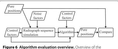
As has been shown in the previous sections, there is a set of algorithm control parameters, which need to be set for the algorithm to work. An iterative DOE approach in which parameters are screened, typically not full factor experimental matrices, and frozen out if not important for the calculated performance response has been used. The algorithm is made self-evaluating (see Figure 6) by sim-ulating the inspection. The inspection simulation output, a rotational sequence of simulated radiographs, is input to the algorithm, and its performance is evaluated for a number of such simulated inspections.
Figure 6Algorithm evaluation overview.Overview of the evaluation of the whole algorithm.
control factors. A noise factor consists of two sets of min and max values for a list of radiograph sequence simulation control factors. Each set of min and max values represents one level of the noise factor. As can be seen in Table 1, three different noise factors at two levels (NF low and high) are used:cnr, geo, anddet. The cnr represents the inherent statistical nature of radiographic inspection. It consists of the two main CNR controlling parameters, D and S, in the X-ray system model. They control the ratio of high to low spatial frequency noise in the radiographs and the overall noise level. Thegeo rep-resents process variation in the weld geometry. The high level reproduces a variation similar to the weld class with medium geometry requirements. Finally, the det con-sists of the width of the detector point spread function, with Lorentzian shape. The X-ray detector is not further
specified apart from its pixel size, which is set to 0.05 mm. For a detailed discussion on the noise parameters and the X-ray model together with its restricted validity range, see [14,22]. The performance evaluation should be inter-preted as a performance indication due to the rather unspecified X-ray setup, with its advantage of a potentially high degree of generalization, and the simplified synthetic radiograph model.
The simulation of a single inspection of a single weld with pores consists of a sequence of radiographs taken at different rotations. The sequence is denoted as rscan for rotational scan. The rotation angles, amplitude and count, as given in Table 1 are chosen for the inspection procedure to be industrially feasible and without any other optimiza-tion. A large amount of rscans is then pre-generated and grouped together in sets having the same noise factor set-tings. These groups will have different amount of inherent variation. The control factors belonging to a noise factor all have their values set to random numbers. The ran-dom numbers are drawn from uniform distributions with ranges set to either NF low or NF high as indicated in Table 1. For example,geoequals H indicate that for those rscans the width parameter (B) on the source side has been uniformly random-sampled within 2.6 to 3.4 mm and so on. Finally, for each rscan, a unique set of pore positions and sizes are randomly sampled from a uni-form distribution (see Table 1). The position distribution
Table 1 Radiograph simulation parameters and noise factors
Grouping Parameter Unit NF Fixed at NF low NF high
Pores Min interspacing mm 0.35
Count 8
Positions mm Uniform random
Min to max radius mm
Weld Plate thickness(T) mm 5
Width(B)DS mm geo 12 5±1
Reinforcement(δ0)DS mm geo 1.5 0.75±0.2
Undercut(δ1)DS mm geo 0.5 0.75±0.2
Width(B)SS mm geo 8 3±0.4
Reinforcement(δ0)SS mm geo 0.8 0.55±0.2
Undercut(δ1)SS mm geo 0.4 0.55±0.2
Setup SDD mm 600
ODD mm 25
Rotation angle(ω) degrees 0, 5, 10, 15, 20, 25
Rotation point(Rx) mm 567
X-ray Attenuation mm−1 0.124
D cnr 110 160
S cnr 6, 000 12, 000
PSF width (σdet) pixel det 0.93 0.93±0.08
is limited by a minimum allowed interspacing between the pores.
The algorithm control parameters are varied in an experiment matrix followed by a performance measure-ment. For each matrix row, the algorithm is run for a small number of different rscans to get some variation in the input. This is essential since the main difficulty is to han-dle the variation in the input, not a limited number of special cases.
The setup of the algorithm control parameters is sep-arated and suboptimized with the segmentation and the tracker screened one at a time. Two responses are used to set up and compare the different segmentation meth-ods. The overall aim is to find as many pores as possible but even more so to know that no pores larger than some defined size is missed. In addition, the tracker will be able to handle some missing measurements for each pore (ilost). One might argue that a good measure of the segmentation performance is the averaged worst case sce-nario. Therefore, the rotational probability of a hit is used as one of the responses and defined as
POHrot≡ min(POHp)rscans, (14)
where POHp = TP/N with TP being the true-positive count for porepover all theNrotations, and POHrot×N is the number of rotation radiographs a pore is detected in. Another relevant response is the measure of the cost of detecting the TPs in terms of the number of false pos-itives per rotation FProt≡ FPrrotationsrscans, where FPr is the total false-positive count for each rotation when TP is maximized.
For both the above responses, each pixel output by the merger procedure, which is the last step in the segmen-tation algorithm, must be classified as either a TP or FP. The merger procedure is set to retrieve at most Cn number of the highest valued pixels from the correlation image, referred to as candidate pores. In addition, the ground truth is known since the expected pixel coordi-nates for each pore can be calculated using Equation 8. To associate each true pore projection with one candidate, a simple nearest neighbor approach with no re-sampling is used. First, the real euclidian distances between each true known pore and allCn candidates are calculated. This is followed by iteratively selecting the pair with the smallest interspacing distance until all p true pores are associ-ated with one-pore candidates. The associassoci-ated pairs might not be unique, but the method is simple and fast and is believed to be a good measure on the average. Finally, to be considered a TP, the distance to the nearest true pore should be less than 1.2 pixel; the threshold is chosen to be slightly larger than 1 pixel.
The tracker is set up and evaluated by setting the last threshold T2 high enough to ensure that all candidates that made it through the tree pruning are present. Each
pore candidate consists of its real 3-D coordinates, which are compared with the known exact positions using the same nearest neighbor approach as in the segmentation evaluation. The candidate is then considered a TP if the distance to the closest true pore is less than a predefined threshold (0.25 mm). If at this stage all pores are found (TP = P), a measure of the relative performance of the settings used in the algorithm is the separation of the scores for the TP and FP classifications. The concept of sensitivity, a measure of separation, is introduced in this context as
Sensitivity= scoreTP− scoreFP s2TP+s2FP
, (15)
where the averages are over all pores in all rscans at the same time, and the s denotes the standard deviation of each of the groups. This is equivalent to the statistic used in common statistical hypothesis testing; note also its sim-ilarity to the Taguchi signal to noise ratio (see for example [21]). Two critical assumptions made are that the stan-dard deviation is a good measure of the relative spread in the data and that the score distribution shape is approxi-mately constant. One possible cost for finding a lot of the pores and maximizing sensitivity is the precision in their 3-D positions. Therefore, the error in positioning is added as a response. The error is defined as the distance between the true 3-D position (input to the simulation) and the one retrieved as a result from the tracker. The spread in the errors is then accounted for when constructing the scalar response by approximating and setting it to the 97th sample quantile [23] of the error in position using all the TPs.
Both the decision on TP and FP at the segmentation setup and the state model in the Kalman filter is based on a simplified but very similar X-ray interaction model as the model used for synthetic radiographs. Therefore, both the segmentation and tracker evaluation could poten-tially contain an inverse crime [24], but they do not since statistical noise is added to the radiographs.
3.1 Probability of a hit
Assumptions are made on the POD curve shape and underlying statistical distributions in order to facilitate an effective approximation of the confidence intervals, assumptions which are unrealistic for this automatic NDE system. Others [27] try to approximate the confidence intervals with the use of sophisticated DOE methods com-bined with less strict assumptions on the NDE system. However, in this article, the POD and the 95% lower confidence interval (POD95) methods of [28] is used.
In [28], the hit/miss formulation is used, where each defect is either detected (hit) or not detected (miss). As already noted in the previous section, in the present work, a hit is defined as detecting and 3-D positioning of a pore to an accuracy of 0.25 mm. Anything else is a miss or a false positive. This threshold is set to less than the min-imum pore interspacing (see Table 1) but large enough to be a relevant length scale. The probability of a hit is used and defined as POH=TP/P, and used to discrim-inate it from the usual meaning of the POD. Assuming that each pore has the same POH as all the other pores in the same range interval, the binomial distribution can be used as in [28]. The main advantage in using the bino-mial approximation is that the confidence intervals can be estimated from TP andPusing standard methods and implementations.
In order to get a high confidence in the POH using few defects, the optimized probability method [28] has been used. The method is outlined here for completeness (see [28] for details). Iteratively, for one radius range at a time, a set of POHs at a lower confidence level of 95% (POH95) is calculated by including one lower radius interval at a time into the calculation. For each radius range, the POH95 is set to the largest of these POH95s. A critical assumption is that the true detectability increases with increased defect size. Curves produced using the optimized method will in general extend the high POH region into lower sizes but at the same time be conservative.
The false detection rate FDR=FP/(FP+TP)is used as a measure of false alarms. This is believed to be relevant since the pore distribution output from the tracker and in the future input to the fatigue life model will consist of FP+TP number of pores.
3.2 Size measurement
A robust scalar measure of the error in size measurement is used to compare different size measurement methods. The ground truth for the size of each pore is known together with the projection coordinates in each radio-graph output from the tracker algorithm. The error mea-sure is constructed by first calculating theU as given in Equation 13 for each pore in each rotation in all rscans. Pairs of a known radius together with a calculated U is produced. The radius is discretized into a number of radius intervals [r − r,r], where r is a parameter
indicating the required resolution. For each radius inter-val, the range ofUis calculated [U0,U1]. This is followed by selecting the set of all radiusRhavingU0≤U≤U1, in order to calculate the new radius interval range asR+ = max(R)−randR−=min(R)−r. Finally, the scalar mea-sure of the relative performanceE=E++E−is calculated by summing overNradius intervalsriaccording to
Ek=
wherek= ±. A high performance is indicated byEbeing close to 1. It should be noted that the method makes no assumptions on the shape of the correlation betweenU and the radius and also accounts for the outliers.
4 Simulation results
This section is both an example of the setup and evalua-tion methodology presented in the previous secevalua-tion and a description of the simulation results. In the setup and evaluation, the algorithm is divided into three parts and performed in the following order: the segmentation, the tracker, and the size measurement. Each part is optimized and evaluated with all the other parts of the algorithm fixed at optimum performance.
4.1 Segmentation
All three segmentation methods are individually opti-mized in order to select the one with the highest per-formance. For each segmentation method and for each control parameter row in the experimental matrix (con-figuration), all four combinations of the (L) and (H) of the noise factors geo andcnrare evaluated. The best result for each method and noise factor combination is presented in Table 2, where the best result is defined by maximizing POHrot, followed by minimizing FProt if there is more than one configuration with the maximum POHrot. The best configuration chosen this way will typ-ically be different for each of the four different noise factor combinations. The main conclusion from Table 2 is that the cross correlation with energy term method have the lowest performance (POHrot ×6 = 2.8 at geo = H,cnr = L), and it is therefore excluded from further considerations.
Table 2 Segmentation methods screening
cnr geo Method POHrot×6 FProt
L L Corr 4.0 104
L L Radial 4.5 320
L L Corr energy 4.0 160
H L Corr 3.8 80
H L Radial 5.5 16
H L Corr energy 5 24
L H Corr 3.0 440
L H Radial 5.0 400
L H Corr energy 2.8 560
H H Corr 3.4 400
H H Radial 5.3 24
H H Corr energy 4.0 480
Cnis fixed at 450 forgeo=Land 600 forgeo=H. Corr, cross correlation; Corr energy, cross correlation with energy as given by Equation 7; Radial, radial symmetry.
rcc = 0.1 mm. The best radial symmetry method config-uration isrrs = 1 px and 2 px,irs = 2,nrs = 1,lrs = 1, andσrs = 1.55 px. As can be seen, in the optimal radial symmetry method configuration, the DST is not active but only the symmetry differential operatorE.
A more detailed performance evaluation is conducted on the radial symmetry method, which was the best seg-mentation method. In Table 4, the effect on POHrotand FProt when extending the pore radius range down to 0.055 mm and changing thecnrlevels can be seen. The CNR for the 0.055 mm pore is roughly CNR ≈ 1±1 for cnr=Land CNR≈7±1 forcnr=H. The segmen-tation is evaluated using the same experimental matrix as used in Table 3, and the optimum configuration is veri-fied to be the same. Furthermore, the conclusion is that for the current radius range, the change in POHrotis mainly due to the change in CNR and the noise spatial frequency
Table 3 Segmentations methods with constant control parameters
cnr geo Method POHrot×6 FProt
L L Corr 3.3 280
L L Radial 4.3 360
H L Corr 3.0 280
H L Radial 5.5 104
L H Corr 2.8 520
L H Radial 5.0 400
H H Corr 3.3 520
H H Radial 5.0 24
Results for the segmentation algorithm with constant segmentation control parameters for each method. The notation is the same as in Table 2.
Table 4 Radial symmetry segmentation at different CNR
cnr S D Radius POHrot FProt
[ 104] (mm) [ 6]
L 2.4 160 0.055 3.8 280
L 2.4 160 0.085 4.8 16
L 2.4 160 0.10 6.0 0
M 5 270 0.055 5.3 168
H 8 350 0.055 6.0 0
Results for segmentation method radial symmetry when changing the minimum pore radius and the CNR (cnr). The radius represent the minimum radius in the pore distributions, and the max radius is fixed at 0.13 mm.
characteristics (differentcnr), rather than the change in spatial size of the 2-D indication.
4.2 Tracking
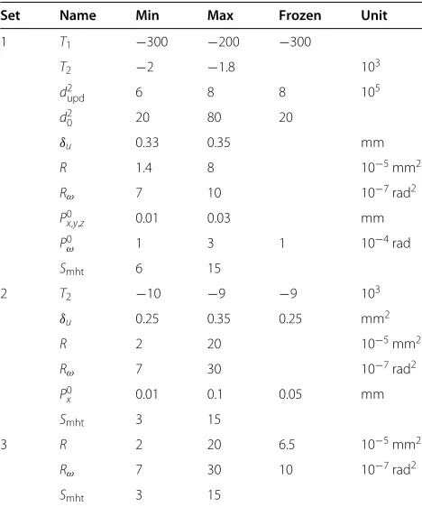
The tracker part of the algorithm is optimized and eval-uated with the segmentation control parameters fixed. The two optimized responses are the sensitivity and the 97th quantile of the positioning error. First, an iterative approach using DOE screening and space filling experi-mental matrices is conducted. The number of rows in the experimental matrix (configurations) for sets 1, 2, and 3 in Table 5 are 15, 40, and 60. Each configuration is evaluated
Table 5 Tracker DOE iterations
Set Name Min Max Frozen Unit
1 T1 −300 −200 −300
T2 −2 −1.8 103
d2
upd 6 8 8 105
d2
0 20 80 20
δu 0.33 0.35 mm
R 1.4 8 10−5mm2
Rω 7 10 10−7rad2
P0
x,y,z 0.01 0.03 mm
P0ω 1 3 1 10−4rad
Smht 6 15
2 T2 −10 −9 −9 103
δu 0.25 0.35 0.25 mm2
R 2 20 10−5mm2
Rω 7 30 10−7rad2
P0
x 0.01 0.1 0.05 mm
Smht 3 15
3 R 2 20 6.5 10−5mm2
Rω 7 30 10 10−7rad2
Smht 3 15
Overview of the iterative DOE approach leading to, in this case, one sensitivity control parameterSmht. Frozen refers to fixed value after conclusions were
drawn using the responses of the active set. The parametersP0
x,P0y,P0z,S0ωare the
Normalized control factor
Figure 7Tracker parametersRandSmht.Correlations found in set 3 as the result of sets 1 and 2 in Table 5. Each control factor or their combination is normalized by translation and scaling.
on eight rscans. SinceCnis held fixed and POH monitored to be close to 1, the clutter density can be considered con-stant. The gates are also fixed atGz=4 mm,Gy=30 mm, Gx0=565 mm, andGx1 =579 mm. In addition, at most, two measurements are accepted to be lost (ilost=4). The results of the iterative process can be seen in Table 5. As can be seen in Figure 7 in combination with Table 5,R can be frozen out andSmhtis then used to maximize the sensitivity.
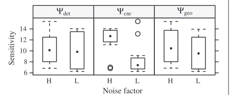
In order to explore which noise factor with the highest effect on the sensitivity, the tracker is evaluated with the noise factors set to difficult one at a time and once for all of them. For each noise factor combination, the tracker is evaluated using two different levels ofSmhtandCT. As can be seen in Figure 8, it is the CNR(cnr)that has the largest effect on the sensitivity, not the width of the detec-tor point spread function(det)nor the process variation in the weld geometries(geo).
In order to set a value onSmht, a full factor experiment onSmhtandCTis executed on a set of rscans with the most difficult noise factors combined (cnr = L,geo = H, det =H). As can be seen in Figure 9, approximately 5 is a good value onSmht. Furthermore, the 97th percentile of the error in positioning is within 0.131 to 0.138 mm.
As a final setup and optimization step, the effect of dif-ferent minimum radii in the pore radius distribution on the performance is explored. Three sets of rscans with
Noise factor
Figure 8Sensitivity for different noise factors.Sensitivity is shown for different combinations of noise factors and two levels onSmhtand
CT.
Figure 9Sensitivity againstSmhtat differentCT.Sensitivity as the
whole algorithm is swept for differentCTandSmht. The data is based
oncnr=L,geo=H, anddet=Hand each point in the plot is
based on 20 rscans.
different minimum pore radii 0.055, 0.085, and 0.1 mm (maximum radius constant at 0.13 mm) are generated. Thecnrsettings are changed toS=24, 000 andD=160. The results based on four rscans can be seen in Figure 10. The higher the sensitivity, the less sensitive toT2(robust) are the POH and FDR and the lower the FDR for a given POH is expected to be. The effect can be seen in the figure as the different behaviors of the two innermost lines (dif-ferentSmht) where theT2 values of the dashed line has been translated and re-scaled for visual comparison.
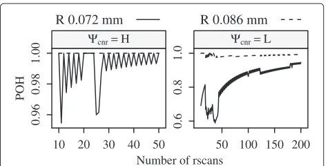
For the purpose of performance evaluation, two new sets of rscans are generated with minimum pore radius 0.055 mm and nonstandard high and low cnr given by S/D = 50, 000/270 and S/D = 30, 000/200. The algo-rithm configuration is the same in both cases withSmht= 5,CT =1.87, and constantT2. The resulting POH95 plot-ted against pore radius is given in Figure 11, where the cnr=H is based on 50 rscans andcnr=L is based on 200 rscans. As can be seen, the POH95 is higher for the cnr = H compared tocnr = L. Furthermore, the con-vergence of the POH for two radius ranges from Figure 11
10 20 30 40 50 60
0.06 0.08 0.10 0.12
0.0
0.4
0.8
Max radius in range [mm]
POH95
Ψcnr=H
Ψcnr=L
Figure 11POH95 against radius.POH95 is calculated using the optimized probability method [28]. The radius intervals are approximately 0.005 mm and the radius taken as the max radius in the interval. The FDR is less than 1%.
as can be seen in Figure 12. Convergence is considered as being reached in both cases since other uncertainties due to the simplified synthetic radiograph model and the unspecified general X-ray setup are assumed to be higher. Finally, the performance in terms of the error in posi-tioning is evaluated. As can be seen in Figure 13, with a q-plot of the error, it is less than 0.05 mm for 80% of the pores in thecnr = L case. In addition, out of the 358 pores which were found in Figure 13, 10 were missing one measurement and 3 were missing two measurements.
4.3 Size measurement
The results for the optimization and selection of the optimum size measurement method are presented in Figure 14. The best configuration is chosen to beF = I2, pre-logarithm on image,rsiz = 2 px, andrme = 10 px. In addition, the performance is evaluated in terms of reso-lution in radius. The resoreso-lution is indicated in Figure 15, which shows the real true radius (known) plotted against the measured radius. However, the X-ray model used does not include scattered radiation, which is assumed to lower this sizing resolution even more.
Number of rscans
Figure 12Convergence of POH.POH against number of rscans for two different radius ranges (R). The range is given as the average radius over the rscan subset and the data is the same as in Figure 11.
f−value
Figure 13Error in positioning.Quantile plot for error in positioning for the radius=0.055 to 0.13 mm case. The graph is based on 50 rscans of thecnr=L case in Figure 11.
5 Experimental setup
The experimental radiographic setup is the same as already illustrated in Figures 1 and 5. It is a conventional radiographic setup with a motorized rotational stage. The X-ray source is a General Electric ISOVOLT 450M2 (Fair-field, CT, USA) with a focus size of 0.4 mm. The radio-graphic setup parameters are held fixed at a tube voltage of 120 kV, current of 5.8 mA, and exposure time of 29 s.
The detector is a high-resolution (pixel size 0.0135 mm) digital detector optimized for high-energy (450 keV) applications (see [29] for details). It is an indirect detec-tor with a scintilladetec-tor connected to a CCD camera. The scintillator-camera connection is a bent fiber optic bun-dle. The bundle introduces detector plane spatial dis-tortions with smooth spatial dependence; however, no corrections are applied.
Four pre-processing steps are applied to the raw radio-graphs. First, the dark-field radiograph, which is the zero
rsiz [px]
Figure 14Optimization of the sizing method.Optimization of errorE+in Equation 16 on the sizing procedure; data is based on 12 rscans containing pores of radius 0.055 to 0.13 mm and using the
cnr=L settings used in Figure 11. The radius intervals are based on
Radius r [mm] Real radius [mm] 0.06
0.08 0.10 0.12
0.0625
0.07
0.0775 0.085 0.0925
0.1
0.1075 0.115 0.1225
0.13
Ψcnr=H
0.0625
0.07
0.0775 0.085 0.0925
0.1
0.1075 0.115 0.1225
0.13
Ψcnr=L
Figure 15Sizing error.Real radius ranges for each radiusr
representing the range [r−0.0075 mm,r], selected using the same algorithm as when calculatingR+andR−. FunctionF=(I)2,
rme=10 px, andI=lnIare applied on the radiograph. Datasets are
the same as in Figure 11.
exposure detector intensity level, is subtracted from the radiograph. Second, a flat-field correction is applied, in which each pixel is divided by its value at exposure of a homogeneous similar body as the one to inspect and multiplied by the average flat-field value. The flat-field correction is necessary since each pixel responds slightly individual to radiation.
Some pixels respond to radiation which is so different compared to the rest that it is required to classify them as noninformation-bearing pixels, the bad pixels. The algo-rithm chosen for bad pixel handling is that of [30] with some minor changes. More sophisticated algorithms have been proposed (see for example [31]), but in this article, a simple bad pixel handling is assumed to be sufficient. Each pixel in the flat field is compared to the median of its neighbors (15×15 px kernel). If the absolute deviation from the median is larger than 2.9 standard deviations, it is classified as a bad pixel. Typically, around 3% are clas-sified as bad (fixed bad pixel map); this is expected and is caused by the special kind of scintillator used. As a third pre-processing step, each pixel labeled as bad is then sub-stituted in the current radiograph by the median value of its neighbors (5×5 px kernel). Often, there are clusters of bad pixels, and of course, any indication at the same size and inside such a cluster would be averaged away. In the fourth and final pre-processing step, the pixels are aver-aged 2×2 into pixel size 0.027 mm (binned) to increase the CNR at the cost of resolution.
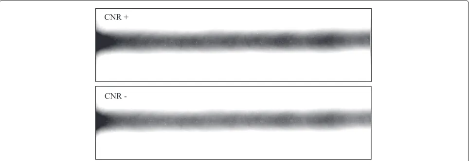
The aim of this work is not to find the most optimal radiographic setup and settings. However, a higher CNR (for example, due to a microfocus X-ray source, differ-ent X-ray energy or exposure time) was indicated (see Section 4) to increase the algorithm performance. There-fore, an experiment on both a high and a low CNR, labeled CNR+and CNR−, is conducted. In the CNR+case, the average over eight exposures at each rotation angle is used;
the average is taken before the first pre-processing step. In the CNR−case, four exposures are instead averaged.
The reference measurement of the sample is made with a commercial CT metrology system, Carl Zeiss Metrotom 800 (Oberkochen, Germany). The sample is a titanium alloy laser weld (Ti-6242, Ti6Al2Sn4Zr2Mo), which is cut out from a large plate into a 5× 10× 30 mm volume. The sample volume is reconstructed with a voxel size (discretized volume size) of 0.018 mm. For large objects, consisting of more than a few voxels, the accuracy and precision in their mass center 3-D position is typically subvoxel. However, for the small objects (the pores) in this article, precision and accuracy are assumed instead to be at the order of the voxel size [32].
6 Experimental results
The radiographic image quality is indicated using a DIN62AL 10 ISO 16 (INTECH NDE, Edmonton, Alberta, Canada) wire penetrameter. The quality is shown in Figure 16 with the penetrameter on the source side of a homogeneous Ti-6242 plate. A faint linear indication of the smallest wire (0.1 mm) can be seen in the CNR+case and the second smallest wire (0.125 mm) in the CNR− case. The detectability of this penetrameter does not indi-cate the detectability of the pores’ 1:1 ratio. However, the overall quality of the radiograph is visualized.
A single rotation radiograph for both CNR cases of the actual weld is shown in Figure 17. The two boxes indicate the selected region of interest, which is held con-stant during the analysis at approximately 900×240 pixel. Horizontal line profiles over three different pore indica-tions from Figure 17 is shown in Figure 18. The CNR is approximately around 2.
Figure 17Experimental radiographs.Experimental radiographs of the weld for both CNR cases. The region of interest is also indicated by the boxes.
The setup geometry as indicated in Figures 1 and 5 is derived using the same procedure, settings, and calibra-tion sample as in [33]. In short, a block of plastic with five ball-bearing steel balls (diameter 0.5 mm) cast inside at different depths andy-zpositions is measured with a CT metrology system. The sample is then inspected with the same radiographic setup as will later be used for the algo-rithm. The steel balls are detected, and an evolutionary algorithm is used to derive a setup geometry parameter set from the known steel ball interspacing positions in 3-D. For details, see [33]. A setup geometry was derived and verified to give approximately 0.1-mm maximum positioning errors. The error was approximated by rerun-ning the analysis discarding the prior knowledge of the steel ball 3-D positions. Referring back to Figure 5, the derived setup geometry parameters used are Rx = 649.9421 mm, Ry = 8.4612 mm, Rz = 12.9290 mm, Sx = 0.0000 mm,Sy = 10.8245 mm,Sz = 13.3204 mm,
CNR −
0
400
CNR +
0 50 100 150 200
0
400
Detector coordinate [px]
Intensity [a.u.]
Figure 18Pore indication line profiles.Three typical line profiles over the pore indications in Figure 17 along the horizontal direction.
and SDD = 717.5830 mm. The object to detector dis-tance ODD ≈ 25 mm; it is however not required by the algorithm and therefore only manually approximated.
The algorithm parameters are held fixed for both the CNR cases. The radial symmetry method is used, and its parameters are the same as the ones used to produce Table 4. The merger parameters are also the same as those used in Table 4 except for the number of pore indica-tions to retrieve in each radiograph, which isCT = 600. Most of the tracker parameter values are the same as the frozen ones in Table 5, except for the final score (probabil-ity) thresholdT2 = 1.8, the intermediate score threshold T1 = −1, 000, the score when no measurement is found d02 = 70, the measurement covariance R = 3.5 × 10⁻⁵mm2, the threshold for merging 3-D positionsδu = 0.08 mm, and the weight when comparing prediction to measured indicationSmht = 3. Theδuhad to be lowered since the pore interspaces in the real samples were lower than assumed.
The nominal thickness of the plate is measured with a mechanical caliper and compared to both CT and the algorithm in this article (abbreviated DR). For both the CT and DR cases, the thickness is measured using three points on one side of the surface to construct a plane; the perpendicular distance to a single point on the other side of the plate is then taken as the thickness. For the DR case, the points consisted of 0.5-mm high-tolerance ball-bearing steel balls, which the algorithm was set up to detect and position. The algorithm parameter values were the same as the for the calibration procedure described in [33]. The result of the three different thickness measure-ments are 4.86±0.02 mm for caliper, 4.93 mm for CT, and 4.73 mm for DR. This indicates an overall magnitude of the error in positioning.
CNR −
CNR +
CT, r ≥ 0.05 mm
CT, r ≥ 0.045 mm
10 15 20 25
2345678
2345678
2
345678
2345678
z [mm]
x [mm]
Figure 19Pore depth (x) against weld length (z) position.The depth coordinatexagainst weld length coordinatezof the pores for DR CNR−and CNR+and CT at two different lower radius thresholds. The weld root enforcement height isδ0≈0.5 mm (caliper), and it is
located on the detector side at high highxcoordinates. Dashed lines indicate the base plate surfaces.
Volume Graphics. Additionally, the diameter and 3-D position of each detected pore are also measured man-ually in the visualization program. The DR pore 3-D position coordinate system is then manually translated and rotated to match the six largest pores from the CT
measurement, a procedure known as registration. The positioning errors between the two point sets (DR and CT) are found to be approximately ≤ 0.1 mm, which is consistent with the validation of the derived setup geometry above. Furthermore, the pore radius range in the reference sample is found to be 0.03 to 0.065 mm, where the smaller radius range POD is assumed to be less than 1.
In Figures 19,20,21,22, the two DR cases, CNR+ and CNR−, are compared to the CT reference measurement. The pore sizes are scaled with an arbitrary number, which is different for CT and DR. In the DR case, the size of each each pore is derived using the same sizing control parame-ters as used in Figure 15 before scaling. Note that the sizes of the pores and aspect ratios between the axes are scaled for visualization, not to reproduce correct scaling. The
CNR −
CNR +
CT, r≥0.05 mm
CT, r≥0.045 mm
10 15 20 25
8
9
10
11
8
9
10
11
8
9
10
11
8
9
10
11
z [mm]
y [mm]
r≥0.05 mm CT DR
r≥0.03 mm
10 15 20 25
2345678
2345678
z [mm]
x [mm]
Figure 21Pore depth (x) against weld length (z) position at different CT radius thresholds.The pore depth coordinatexagainst weld length coordinatezfor both DR CNR+and CT. The radius (r) represents two different lower thresholds in the CT results.
pore 3-D positions measured with the proposed algorithm (DR) agree qualitatively well with the CT reference.
A qualitative POH measurement is indicated in Table 6. Each DR pore is manually matched to one of the CT refer-ence pores and classified as detected, or if no CT referrefer-ence pore is close enough (see Figures 19,20,21,22), it is classi-fied as a false positive. The information in Table 6 should be seen as a rough estimate of where the POH starts to decrease, in this case, at the diameter of approximately 0.1 mm. In addition, as expected, the POH is higher for the CNR+than for the CNR−case. As for the false posi-tives, it can be seen in Figures 21 and 22 that many pores can be mistaken for false positives unless smaller pores are included in the reference measurement. The num-ber of false positives are low when the small pores (r ≥ 0.03 mm) are included. The two pores in the DR cases at x,y,z ≈ 2, 11, 18 mm can be seen as grooves on the surface of the sample. This adds up to in total one false positive in the CNR+case at(x,y,z) ≈ (2.5, 11, 18)mm. Finally, among the pores found in Table 6, three missed one measurement in the CNR+ case and two in the CNR− cases. The conclusion is that the algorithm can detect pores without requiring them to be detected in all projections.
r≥0.05 mm
CT DR
r≥0.03 mm
10 15 20 25
8
9
10
11
8
9
10
11
z [mm]
y [mm]
Figure 22Pore lateral (y) against weld length (z) position at different CT radius thresholds.The pore lateral coordinateyagainst weld length coordinatezfor both DR CNR+and CT. The radius (r) represents two different lower thresholds in the CT results.
7 Conclusions
In this article, an algorithm has been derived to handle the detection, positioning, and sizing of submillimeter-sized pore defects in thin laser-welded titanium inspected with radiography. The algorithm has been set up and pre-evaluated on synthetic radiographs using a DOE method-ology. In addition, it has been qualitatively evaluated on real experimental welds. The algorithm is based on gen-eral tracking theory, in contrast to the previous solutions in literature, which are based on a vision system approach. In addition, it does not require the defects to be detected in all rotation projections. This relaxed demand on detec-tion in all projecdetec-tions is important for detecting low CNR defects with radiographic inspection.
Table 6 Detected pores for both DR and CT
Min radius CT DR CNR+ DR CNR−
(mm) (n) (n) (n)
0.055 6 6 6
0.05 15 14 11
0.045 21 17 14
The qualitative experimental comparison shows good agreement between the 3-D positions found using the proposed algorithm and the computerized tomography reference measurements. In addition, performance evalu-ation on both the synthetic and the experimental radio-graphs indicate that the probability of a hit increases with CNR; hence, as the hardware performance used for inspection will improve in the future, the performance of the algorithm will too. The synthetic and the experimen-tal radiographs both indicate a low false-defect detection rate. However, the defect size measurement part of the algorithm could not be experimentally verified due to very low resolution in the reference measurements.
In the future, a quantitative experimental benchmark of the proposed algorithm and its inspection procedure needs to be conducted. Furthermore, in order to detect and position the defects which are not detected in all projections more efficiently, other trackers or modifica-tions to the multiple hypothesis tracker used here could be interesting to explore.
Competing interests
The author declares that he has no competing interests.
Acknowledgements
This work was done with the financial support from the Swedish National Aeronautical Research Program (NFFP). The Ti-6242 samples from GKN Aerospace and the help with making the CT measurements by Carl Zeiss Measurement Center in Olofström is gratefully acknowledged. The anonymous reviewers are acknowledged for their useful work. The author is thankful for the useful comments on the tracker parts by Associate Professor Lennart Svensson. The author also would like to thank Associate Professor Håkan Wirdelius and Dr. Peter Hammersberg for the help and support with the manuscript.
Received: 16 August 2013 Accepted: 21 January 2014 Published: 25 January 2014
References
1. Y Murakami,Metal Fatigue: Effects of Small Defects and Nonmetallic Inclusions(Elsevier, Amsterdam, 2002)
2. A Haboudou, P Peyre, AB Vannes, G Peix, Reduction of porosity content generated during Nd:YAG laser welding of A356 and AA5083 aluminium alloys. Mater. Sci. Eng. A Struct. Mater.363, 40–52 (2003)
3. MW Turner, PL Crouse, L Li, AJE Smith, Investigation into CO2 laser cleaning of titanium alloys for gas-turbine component manufacture. Appl. Surf. Sci.252, 4798–4802 (2006)
4. S Krimmel, J Baumann, Z Kiss, A Kuba, A Nagy, J Stephan, Discrete tomography for reconstruction from limited view angles in
non-destructive testing. Electron. Notes Discrete Math.20, 455–474 (2005) 5. ER Doering, JP Basart, JN Gray, Three-dimensional flaw reconstruction and
dimensional analysis using a real-time X-ray imaging system. NDT E Int.
26, 7–17 (1992)
6. R Vijay, RS Anand, A comparative study of different segmentation techniques for detection of flaws in NDE images. J. Nondestruct. Eval.
31, 1–16 (2012)
7. R Vilar, J Zapata, R Ruiz, An automatic system of classification of weld defects in radiographic images. NDT E Int.42, 467–476 (2009) 8. RR da Silva, LP Caloba, MHS Siqueira, JMA Rebello, Pattern recognition of
weld defects detected by radiographic test. NDT E Int.37, 461–470 (2004) 9. TW Liao, DM Li, YM Li, Detection of welding flaws from radiographic
images with fuzzy clustering methods. Fuzzy Sets Syst.108, 145–158 (1999)
10. D Mery, D Filbert, Automated flaw detection in aluminium castings based on the tracking of potential defects in a radioscopic image sequence. IEEE Trans. Robotics Automation.18, 890–901 (2002)
11. M Carrasco, D Mery, Automatic multiple view inspection using geometrical tracking and feature analysis in aluminum wheels. Mach. Vis. Appl.22, 157–170 (2011)
12. J Shao, D Du, B Chang, H Shi, Automatic weld defect detection based on potential defect tracking in real-time radiographic image sequence. NDT E Int.46, 14–21 (2012)
13. S Blackman, R Popoli,Design and Analysis of Modern Tracking Systems
(Artech House, Norwood, 1999)
14. E Lindgren, H Wirdelius, Separation of geometrical- and defect information in digital radiographs using wavelet techniques, in20th ISABE Conference 2011 Proceedings(AIAA, Reston, 2011), p. 1616
15. VD Gesu, C Valenti, Symmetry operators in computer vision. Vistas Astron.
40, 461–468 (1996)
16. VD Gesu, R Palenichka, A fast recursive algorithm to compute local axial moments. Signal Process.81, 265–273 (2001)
17. D Comaniciu, P Meer, Mean shift: a robust approach toward feature space analysis. IEEE Trans. Pattern Anal. Mach. Intell.24, 603–619 (2002) 18. RG Brown, PY Hwang,Introduction to Random Signals and Applied Kalman
Filtering(John Wiley & Sons, New York, 1997)
19. DB Reid, An algorithm for tracking multiple targets. IEEE Trans. Automat. Contr.AC-24, 843–854 (1979)
20. G Demos, R Ribas, T Broida, S Blackman, Applications of MHT to Dim moving targets. SPIE Signal Data Process. Small Targets.1305, 297–309 (1990)
21. B Bergman,Industriell försöksplanering och robust konstruktion
(Studentlitteratur AB, Lund, 1992)
22. E Lindgren, H Wirdelius, X-ray modeling of realistic synthetic radiographs of thin titanium welds. NDT E Int.51, 111–119 (2012).
[doi:10.1016/j.ndteint.2012.06.007]
23. RJ Hyndman, Y Fan, Sample quantiles in statistical packages. Am. Stat.
50, 361–365 (1996)
24. D Colton, R Kress,Inverse Acoustic and Electromagnetic Scattering Theory
(Springer, Heidelberg, 1992). [Chap. 5.3]
25. A Berens, NDE reliability data analysis, inASM Metals Handbook: Nondestructive Evaluation and Quality Control,9th edn, vol. 17 (ASM, New York, 1989), pp. 689–701
26. US Department of Defense,MIL-HDBK-1823A: Nondestructive Evaluation NDE System Reliability Assessment(US Department of Defense, Washington, DC, 1999)
27. E Generazio, Design of experiments for validating probability of detection capability of NDT systems and for qualification of inspectors, inMaterials Evaluation(American Society for Nondestructive Testing, Columbus, 2009), pp. 730–738
28. B Yee, F Chang, J Couchman, G Lemon,NASA-CR-134991: Assessment of NDE Reliability Data(National Aeronautics and Space Administration, Washington, DC, 1976)
29. L Hammar, Novell design of high resolution imaging x-ray detectors, in
18th World Conference in Nondestructive Testing,Durban, 16–20 April 2012 30. C Sabbey, R McMahon, J Lewis, M Irwin, Infrared imaging data reduction
software and techniques, in18th World Conference in Nondestructive TestingDurban, 16–20 April. Astronomical Society of the Pacific Conference Series, vol. 238 (Astronomical Society of the Pacific, San Francisco, 2001)
31. S Ghosh, D Froebrich, A Freitas, Robust autonomous detection of the defective pixels in detectors using a probabilistic technique. Appl. Optics.
47, 6904–6924 (2008)
32. S Carmignato, A Pierobon, P Rampazzo, M Parisatto, E Savio, CT for industrial metrology - accuracy and structural resolution of CT dimensional measurements, inConference on Industrial Computed Tomography (ICT),Wels, 19–21 September 2012
33. E Lindgren, L Hammar, Evaluation of an automatic system for detection and position of small pore defects using digital radiography. AIP Conf. Proc.1511, 1646–1653 (2013)
doi:10.1186/1687-6180-2014-9

![Figure 15 Sizing error. Real radius ranges for each radius rrepresenting the range [ r − 0.0075 mm, r], selected using the samealgorithm as when calculating R+ and R−](https://thumb-us.123doks.com/thumbv2/123dok_us/899592.1108434/13.595.57.292.89.219/figure-sizing-radius-ranges-rrepresenting-selected-samealgorithm-calculating.webp)