R E S E A R C H
Open Access
Rate distortion performance analysis of nested
sampling and coprime sampling
Junjie Chen
1*and Qilian Liang
1,2Abstract
In this paper, rate distortion performance of nested sampling and coprime sampling is studied. It is shown that with the increasing of distortion, the data rate decreases. With these two sparse sampling algorithms, the data rate is proved to be much less than that without sparse sampling. With the increasing of sampling spacings, the data rate decreases at certain distortion, which is because with more sparse sampling, less number of bits is required to represent the information. We also prove that with the same sampling pairs, the rate of nested sampling is less than that of coprime sampling at the same distortion. The reason is that nested sampling collects a little less number of samples than coprime sampling with the same length of data, which is a little sparser than coprime sampling.
Keywords: Sparse sampling; Rate distortion; Information theory; Nested sampling; Coprime sampling
1 Introduction
The twenty-first century is awash with data. Data are flooding in at rates never seen before, doubling almost every 18 months [1], as result of new information gathered from Radar, Web communities, newly deployed smart assets, and customer data from public, proprietary, pur-chased sources, and so forth. For example, oil companies, telecommunication companies, and other data-centric industries have had huge data for long time. Data is being collected and transmitted at unprecedented scale [2,3] in a wide range of application areas nowadays. The phrase ‘Big Data’ as defined by US National Science Foundation in its recent solicitation, refers to large, diverse, complex, distributed data sets generated from instruments, sensors, Internet transactions, email, video, click streams, and all other digital sources available today and in the future.
Unstructured data is data that does not follow a speci-fied format, which is really most of the Big Data. Radar or sonar data is one typical example, which includes meteo-rological, vehicular, and oceanographic seismic informa-tion, such as in [4], Big Data from O’Reilly radar was described.
And many efforts have been made to develop suitable compression techniques for Big Data. However,
tradi-*Correspondence: [email protected]
1Department of Electrical Engineering, University of Texas at Arlington, 416 Yates St, Arlington, TX 76019, USA
Full list of author information is available at the end of the article
tional compression methods [5,6] are all based on Nyquist rate, which will have poor efficiency in terms of both sampling rate and computational complexity. Unlike tra-ditional compression techniques, some sparse sampling algorithms have been proposed to overcome Nyquist sampling requirement, like compressive sensing, nested sampling, and coprime sampling.
Nested sampling [7] is an non-uniform sampling, using two different samplers in each period. Although the signal is sampled sparsely and non-uniformly, the autocorrela-tion of signal could be estimated at all lags. Therefore, although the samples can be arbitrarily sparse, it keeps the signal’s statistical information [8]. While coprime sam-pling uses two uniform samplers, with sample spacingsP andQcoprime integers. The authors in [8] have already proved that these two sets of samples of the signal could fully estimate all lags of autocorrelation of the original sig-nal. As both nested sampling and coprime sampling could keep the statistical property of the original signal, these two sampling algorithms could be applied to Big Data to highly reduce the transmission or storage cost of Big Data. Information rate distortion function is a measure of dis-tortion between the original source and its representation. In this paper, we will provide theoretical rate distortion performance, because of these two sparse sampling algo-rithms, either nested sampling (NS) or coprime sampling (CS). We will show that with these two sparse sampling algorithms, the data rate is much less than that without
sparse sampling for a given distortion. With the increas-ing of samplincreas-ing spacincreas-ings, the data rate decreases at certain distortion, which is because with more sparse sampling, less number of bits is required to represent the informa-tion. We will also prove that with the same sampling pairs, the rate of nested sampling is less than that of coprime sampling at the same distortion.
The rest of this paper is organized as follows. In Section 2, we give a brief introduction of nested sampling and coprime sampling separately. Theoretical derivation of rate distortion performance of nested sampling and coprime sampling is detailed in Sections 3.1 and 3.2. Also, the theoretical analysis and comparison of these two sparse sampling is given in Section 3.3. In Section 4, numerical results are provided to verify the theoretical rate distortion results derived in Section 3. Conclusions are given in Section 5.
2 Preliminaries
2.1 Nested sampling
The nested array was first introduced in [7] as an effec-tive approach to array processing with enhanced degrees of freedom [9,10]. In time domain, the signal’s autocor-relation could also be obtained from nested sampling structure [11]. And although the samples from this nested sparse sampling are sparsely and non-uniformly located, the samples of the autocorrelation can be computed at any specified rate. Some applications which depend on the difference co-array, or autocorrelation, like Direction-of-arrival (DOA) estimation and beamforming could be done based on nested sampling.
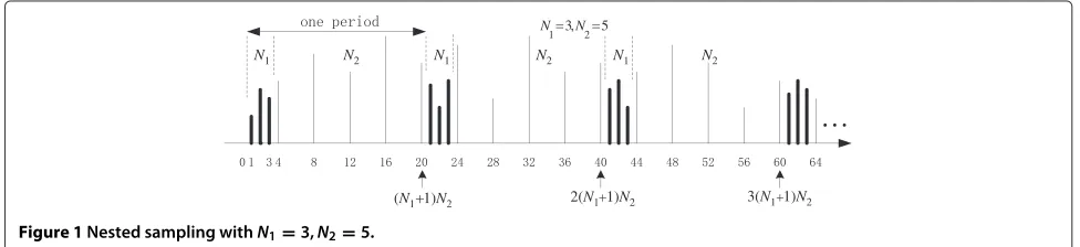
In the simplest form, there are two levels of sampling density in nested sampling [11-14], with the level 1 sam-ples at theN1locations and the level 2 samples at theN2 locations.
1≤l≤N1, for level 1
(N1+1)m, 1≤m≤N2, for level 2
An example of periodic sparse sampling using nested sampling structure is shown in Figure 1, withN1=3 and N2=5. The cross differences are given by
k=(N1+1)m−l, 1≤m≤N2, 1≤l≤N1. (1)
The cross differences (2) are in the following range with the maximum value (N1+ 1)N2 − 1 [9,11], except the integers and the corresponding negated versions shown in (3).
−[(N1+1)N2−1]≤k≤[(N1+1)N2−1] (2)
(N1+1), 2(N1+1),· · ·,(N2−1)(N1+1) (3)
For example, consider the example in Figure 1, where N1 = 3,N2 = 5, 1 ≤ m ≤ 5 and 1 ≤ l ≤ 3, the cross differencesk=(N1+1)m−lwill achieve these values
1, 2, 3,(), 5, 6, 7,(), 9, 10, 11,(), 13, 14, 15,(), 17, 18, 19.
The difference 0 is also missing, for the reason thatm andl are nonzero. Meanwhile, we notice that all of the missing differences could be covered by the self differ-ences among the second array,
(N1+1)(m1−m2), 1≤m1,m2≤N2. (4)
Combining the cross differences and the self-differences is the difference-array, which is a filled difference co-array as shown in (2). This indicates that using nested array structure, although sparse samples are obtained, the degrees of freedom is enhanced,
2[(N1+1)N2−1]+1=2(N1+1)N2−1. (5)
Based on the principle above, a sparse non-uniform sampling using nested sampling structure could be per-formed as in Figure 1. There are two levels of nesting, with N1level-1 samples andN2level-2 samples in each period, with period(N1+1)N2. It is obvious that nested sampling is non-uniform and the samples obtained are very sparse.
We could notice that, in(N1+1)N2Tseconds, there are totallyN1+N2samples. Therefore, the average sampling rate is
fs,nested=
N1+N2 (N1+1)N2T ≈
1 N1T +
1 N2T
< 1
T (6)
Here, T = 1/fn, fn ≥ 2fmax is the Nyquist sam-pling frequency. As the Nyquist samsam-pling rate is 1/T, the
N1 N2 N1 N2 N1 N2
1)N2
2(N1 3(N11)N2
1)N2
(N1
5 , 3
2 1 N N
average sampling rate of nested sampling is smaller than the conventional Nyquist sampling rate.
2.2 Co-prime sampling
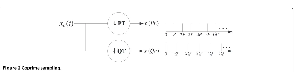
Different from nested sampling, coprime sampling involves two sets of uniformly spaced samplers [8,12-14] as shown in Figure 2, each of them are sparsely sampled.
The coprime sampling uniformly sample the source sig-nal using two sub-Nyquist samplers, with sample spacing PT and QT respectively, where P and Q are coprime integers withP<Q. 1/THz is the Nyquist rate for a ban-dlimited process, i.e., 1/T =2fmax,fmaxbeing the highest frequency.
x(n)=xc(nT). (7)
Consider the product
x(Pn1)x∗(Qn2), (8)
where x(Pn1) and x(Qn2) comes from the first and the second sampler. Let the difference as
k=Pn1−Qn2. (9)
It has been shown thatkcan achieve any integer value in the range 0≤k≤PQ−1 in [11], ifn1andn2are in the ranges 0≤n1≤2Q−1 and 0≤n2≤P−1.
For coprime sampling, the two samplers totally collect P+Qsamples inPQT seconds, so the average sampling rate is
fs,coprime= P+Q
PQT =
1 PT +
1 QT <
1
T. (10)
Same as in nested sampling,T =1/fn,fn≥2fmaxis the Nyquist sampling frequency. It is obvious the average sam-pling rate of coprime samsam-pling is also much smaller than the conventional Nyquist sampling rate. However, the sig-nal’s second-order statistics, like the autocorrelation, is kept, which allows us to sample a signal sparsely and esti-mate some aspects of the signal (spectra, DOA, and so on) at a significantly higher resolution.
3 Rate distortion performance
Information rate distortion function is a measure of dis-tortion between the original source and its representa-tion. Our purpose is to construct a distortion function
which can measure the distortion because of these two sparse sampling algorithms, either nested sampling (NS) or coprime sampling (CS). Sparse sampling can cause possible distortion because less number of samples are used. A wide variety of distortion functions, such as Euclidean distance, Hamming distance, Mahalanobis dis-tance, and Itakura-Saito distance have been used. In this paper, squared error distortion is used. The original sam-ples are denoted asxi,i = 1,· · ·,L, where Lis the total number of samples. Assume that all original informa-tion fromLsamples isXL =[x1,x2,· · ·,xL], the selected information after sparse sampling can be represented as [15]
ˆ
XL =S(XL), (11)
where S(·) denotes sparse sampling, either nested sam-pling or coprime samsam-pling. XˆL =[xˆ1,xˆ2,· · ·,xˆL] and L<L. The distortion associated with the sparse sampling between all original samples and the selected samples is
D=Ed(XL,XˆL), (12)
whered(·)is the distortion function.
The expectation in (12) is with respect to the probability distribution on XL. The rate distortion function R(D) is the minimum of data ratesRsuch that(R,D)is in the rate distortion region for a given distortion. From [16,17], we know that information rate distortion function is defined as
R(D)= min Ed(XL,XˆL)≤DI
(XL;XˆL), (13)
where I(XL;XˆL) is the mutual information between XL andXˆL.
I(XL;XˆL)=H(XL)−H(XL| ˆXL)
=H(XL)−H(XL− ˆXL| ˆXL)
(a)
≥H(XL)−H(XL− ˆXL),
(14)
where inequality(a)follows from the fact that condition reduces the entropy.
From formula (13), we know that
Ed(XL,XˆL)≤D (15)
PT
QT
x (Pn)
x (Qn)
0
0 P 2P 3P 4P 5P 6P
Q
3
Q
2
Q 4Q 5Q
xc
(
t
)
For squared error distortion,
Since Gaussian assumption is a classical modeling assumption heavily used in areas such as signal process-ing and communication system [18], from [16], the rate distortion function for a single Gaussian sourceN(0,σ2) with squared error distortion is
R(D)=
For L-independent zero mean Gaussian sources x1,· · ·,xL with variance σ12,σ22,· · ·,σL2, the rate distor-tion performance with squared error distordistor-tion is given by [16,17,19,20] This gives rise to a kind of reverse waterfilling. We choose a constant λ and only describe those random variables with variance greater than λ, and no bits are used to describe random variables with variance less thanλ.
3.1 For nested sampling
Theorem 1. (Rate distortion for nested sampling of Gaussian source) Let xi ∼ N(0,σi2), i = 1, 2,· · ·,L, be independent Gaussian random variables, and under squared error distortion. The rate distortion between the original Gaussian source and after nested sampling of these Gaussian random variables is given by
RNS(D)=
Proof 1.For nested sampling (NS), all L original infor-mation is XL=[x1,x2,· · ·,xL].
And less number of samples Lwill be selected based on nested sampling as described,
ˆ
where the length of KNScould be determined based on the following formula, here we assume Y =L(mod(N1+1)N2)
If all samples are assumed to be independent Gaussian N(0,σi2), hence, the corresponding rate distortion function for nested sampling will be
RNS(D)= min
where inequality (c) follows from the fact that the nor-mal distribution maximizes the entropy for a given second moment, andKNS
k=1Dk =D.
and differentiating with respect to Dk and setting equal to
which results in an equal distortion for each random vari-able, if the constant λ is less than σi2 for all i. As the increase of the total allowable distortion D, the constant λ increases until it exceeds σi2 for some i. Kuhn-Tucker conditions could be used to find the minimum in (26) if we increase the total distortion D. In this case, the Kuhn-Tucker conditions yield
3.2 For coprime sampling
Theorem 2.(Rate distortion for coprime sampling of Gaussian source) Let xi ∼ N(0,σi2), i = 1, 2,· · ·,L, be independent Gaussian random variables, and under squared error distortion. The rate distortion between the original Gaussian source and after coprime sampling of these Gaussian random variables is given by
RCS(D)=
Proof 2.For coprime sampling (CS), we still assume the original information with length L, i.e., XL = [x1,x2,· · ·,xL].
And based on coprime sampling, less number of samples Lwill be selected,
ˆ
where the length of KCScould be determined based on the following formula
Therefore, the corresponding rate distortion function for coprime sampling of independent Gaussian source N(0,σi2)is
The minimum value could be obtained using the similar procedure as described in nested sampling.
3.3 Theoretical analysis
Without sparse sampling, the rate distortion function would be
which is much greater than that with sparse sampling. From the above derivation of rate distortion function of nested sampling and coprime sampling, we could notice that if the sampling spacings are assumed to be the same, i.e., N1 = P and N2 = Q for these two sparse sam-pling methods, then the minimum value ofKNSmin could
Table 1KNSandKCSwith respect to sampling intervals whenN1=P,N2=Q, andL=1, 000
N1=P N2=Q KNS KCS
3 4 561 500
3 5 600 533
3 7 642 572
3 11 681 607
3 13 690 616
3 17 705 628
3 23 717 638
5 23 794 765
7 23 833 821
11 23 873 870
While for coprime sampling, the minimum value of KCSmin could be achieved when L (modP)=0,
L(modQ)=0, andL(modPQ)=0, therefore
KCSmin=
(P−1)(Q−1)L
PQ =
(P2Q−P2−Q+1)L PQ(P+1) .
(40)
As we know that for these two sparse sampling algo-rithms, the sampling interval is for sure greater than Nyquist sampling spacing, which indicates that Q > 1, therefore,
KNSmin>KCSmin (41)
which indicates that in most cases,KNS > KCS. Table 1 shows some example ofKNSandKCSwith respect to sam-pling intervals whenN1 =P,N2 = Q, andL= 1, 000. It is clear that with the increase of sampling spacings, sam-ples are selected more sparsely by both nested sampling
0.1 0.2 0.3 0.4 0.5 0.6 0.7 0.8 0.9 1 200
400 600 800 1000 1200 1400 1600 1800 2000
D
R(D)
Rate Distortion−Nested Sampling
N1=3,N2=5 N1=3,N2=11 N1=3,N2=17 N1=5,N2=23 N1=11,N2=23
Figure 3Rate distortion performance-nested sampling.
0.1 0.2 0.3 0.4 0.5 0.6 0.7 0.8 0.9 1 200
400 600 800 1000 1200 1400 1600 1800 2000
D
R(D)
Rate Distortion−Coprime Sampling
P=3,Q=5 P=3,Q=11 P=3,Q=17 P=5,Q=23 P=11,Q=23
Figure 4Rate distortion performance-coprime sampling.
and coprime sampling, which results in a increase ofKNS andKCS. In addition, we could notice thatKNS > KCS as proved.
With our assumption that all samples are independent GaussianN(0,σi2), we could conclude that
RNS(D) <RCS(D) <RWS(D) (42)
which indicates that both nested sampling and coprime sampling use less number of bits to describe the informa-tion compared that without sparse sampling (WS).
As we know from the introduction part, in(N1+1)N2T seconds, there are totally N1 + N2 samples for nested sampling, while coprime sampling totally collect P + Q samples inPQT seconds. If the sampling intervals are the same, i.e.,N1 = PandN2 = Q, it is obvious that nested sampling is a little sparser than coprime sampling method.
0.1 0.2 0.3 0.4 0.5 0.6 0.7 0.8 0.9 1 400
600 800 1000 1200 1400 1600 1800 2000
D
R(D)
Rate Distortion
Coprime Sampling, P=3,Q=5 Nested Sampling, N1=3,N2=5 Coprime Sampling, P=3,Q=17 Nested Sampling, N1=3,N2=17 Coprime Sampling, P=5,Q=23 Nested Sampling, N1=5,N2=23
RNS(D) < RCS(D)is because nested sampling collects a little less number of samples than coprime sampling with the same lengthLof data. The rateR(D)at a given dis-tortion for both sparse sampling algorithms is less than that without sparse sampling. The reason is that with sparse sampling, less number of bits is used to describe the original information.
4 Numerical results
The total length of the information is set to beL=1, 000. Each sample is assumed to follow a Gaussian distribution N(0, 1)with zero mean and unit variance. We also assume Dk = λ < σ2 = 1, which is equal distortion for each random variable.
Figure 3 shows the rate distortion performance of nested sampling with different sampling spacings. It is clear that with the increasing of distortion, the rate decreases. When the sampling intervalsN1andN2becomes larger, i.e., less samples are acquired, the rate becomes smaller. For exam-ple, when D = 0.3, N1 = 3,N2 = 5, the data rate R(D) ≈ 1, 350, while with the increase of sampling pairs toN1 = 3,N2 = 11, thenR(D) ≈ 1220, which is much smaller. This is because with more sparse sampling, less number of bits is required to represent the information.
The rate distortion performance of coprime sampling with different sampling spacings is shown in Figure 4. Similarly as nested sampling, with the increasing of distor-tion, the rateR(D)decreases. When the sampling intervals PandQbecomes larger, the rate becomes smaller.
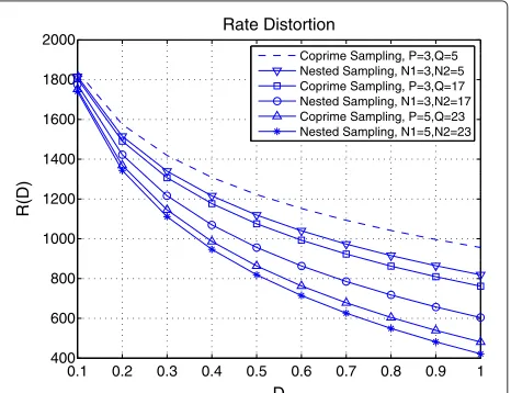
Figure 5 compares the rate distortion performance between nested sampling and coprime sampling, where D is the distortion between the original source and its sparse-sampled representation, and R(D) is the corre-sponding rate at a particular distortionD. With the same sampling spacings chosen,N1 = P, andN2 = Q, at the same distortion, the rate of nested sampling is less than that of coprime sampling. For example, whenN1=P=3, andN2 = Q = 17, whenD = 0.3, the rate for nested sampling isRNS(D) ≈ 1, 200, while the rate for coprime sampling isRCS(D) ≈ 1, 300. This verifies the result that RNS(D) <RCS(D), because nested sampling collects a lit-tle less number of samples than coprime sampling with the same lengthL of data, which is a little sparser than coprime sampling.
5 Conclusions
Information rate distortion function is a measure of dis-tortion between the original source and its representation. Our purpose in this paper is to construct a distortion func-tion which can measure the distorfunc-tion because of these two sparse sampling algorithms. Information theoretical rate distortion performance for these two sparse sampling methods, nested sampling and coprime sampling, is stud-ied in this paper. It is showed that with these two sparse
sampling algorithms, the data rate is proved to be much less than that without sparse sampling at a given distor-tion. With the increasing of sampling spacings, i.e., data are more sparsely acquired, the data rate decreases at cer-tain distortion. This is because with sparser sampling, less number of bits is required to represent the information. We also show that with the same sampling pairs, the rate of nested sampling is less than that of coprime sampling at the same distortion.
Competing interests
The authors declare that they have no competing interests.
Acknowledgements
This work was supported in part by US Office of Naval Research under Grants N00014-13-1-0043, N00014-11-1-0865, US National Science Foundation under grants CNS-1247848, CNS-1116749, CNS-0964713, and National Science Foundation of China (NSFC) under grant 61372097.
Author details
1Department of Electrical Engineering, University of Texas at Arlington, 416
Yates St, Arlington, TX 76019, USA.2College of Electronic and Communication
Engineering, Tianjin Normal University, Tianjin 300387, China.
Received: 16 November 2013 Accepted: 15 January 2014 Published: 10 February 2014
References
1. J Bughin, M Chui, J Manyika,Clouds, Big Data, and Smart Assets: Ten Tech-enabled Business Trends to Watch, vol. 56. (McKinsey Quarterly, New York, 2010), pp. 75–86
2. A Labrinidis, HV Jagadish, Challenges and opportunities with big data. Proc. VLDB Endowment.5(12), 2032–2033 (2012)
3. D Bollier, CM Firestone,The Promise and Peril of Big Data(Aspen Institute, Communications and Society Program, Washington, DC, 2010) 4. O’Reilly Radar Team,Big Data Now: Current Perspectives from O’Reilly Radar
(O’Reilly Media, Sebastopol, 2011)
5. J Chen, Q Liang, J Paden, P Gogineni, inProceedings of the IEEE International Conference on Communications (ICC’12). Compressive sensing analysis of synthetic aperture radar raw data (Ottawa, ON, 10–15 June 2012), pp. 6362–6366
6. J Chen, Q Liang, Efficient sampling for radar sensor networks. Int. J. Sensor Netw., in press
7. P Pal, PP Vaidyanathan, Nested Arrays: a novel approach to array processing with enhanced degrees of freedom. IEEE Trans. Signal Process.
58(8), 4167–4181 (2010)
8. P Pal, PP Vaidyanathan, inProceedings of the Digital Signal Process. Workshop, IEEE Signal Process. Educ. Workshop. Coprime sampling and the MUSIC algorithm (Sedona, AZ, 4–7 January 2011), pp. 289–294
9. P Pal, PP Vaidyanathan, inProceedings of the Acoustics Speech Signal Process. A novel array structure for directions-of-arrival estimation with increased degrees of freedom (Dallas, TX, 14–19 March 2010), pp. 2606–2609 10. P Pal, Piya, PP Vaidyanathan, inProceedings of the IEEE Int. Conf. Acoustics,
Speech Signal Process. (ICASSP). Two dimensional nested arrays on lattices (Prague, 22–27 May 2011, 2011), pp. 548–2551
11. PP Vaidyanathan, P Pal, Sparse sensing with co-prime samplers and arrays. IEEE Trans. Signal Process.59(2), 573–586 (2011)
12. J Chen, Q Liang, B Zhang, X Wu, Spectrum efficiency of nested sparse sampling and co-prime sampling. EURASIP J. Wireless Commun. Netw.
2013, 47 (2013)
13. J Chen, Q Liang, J Wang, H-A Choi, inWireless Algorithms, Systems, and Applications. Spectrum efficiency of nested sparse sampling (Springer, Berlin Heidelberg, 2012), pp. 574–583
14. J Chen, Q Liang, J Wang, Secure transmission for big data based on nested sampling and coprime sampling with spectrum efficiency. Secur. Commun. Netw. Wiley Security Comm. Networks (2013).
15. Q Liang, X Cheng, SC Huang, D Chen, Opportunistic sensing in wireless sensor networks: theory and application. IEEE Trans. Comput. (2013). doi:10.1109/TC.2013.85
16. TM Cover, JA Thomas,Elements of Information Theory, Second Edition. (Wiley, Hoboken, 2006)
17. J Chen, Q Liang, inProceedings of the IEEE Global Telecommun. Conf. (GLOBECOM 2011). Rate distortion performance analysis of compressive sensing (Houston, TX, 5–9 December 2011), pp. 1–5
18. M Capdevila, OWM Florez, A communication perspective on automatic text categorization. IEEE Trans. Knowl. Data Eng.21, 1027–1041 (2009) 19. J Chen, Q Liang, B Zhang, X Wu, Information theoretic performance
bounds for noisy compressive sensing. Paper presented at the ICC’2013, Budapest, 09–13 June 2013
20. J Chen, Q Liang, Theoretical performance limits for compressive sensing with random noise. Paper presented at the IEEE Global Communications Conference 2013 (GLOBECOM’13), Atlanta, 09–13 December 2013
doi:10.1186/1687-6180-2014-18
Cite this article as:Chen and Liang:Rate distortion performance analysis of nested sampling and coprime sampling.EURASIP Journal on Advances in Signal Processing20142014:18.
Submit your manuscript to a
journal and benefi t from:
7Convenient online submission 7Rigorous peer review
7Immediate publication on acceptance 7Open access: articles freely available online 7High visibility within the fi eld
7Retaining the copyright to your article