Application of scattering theory to P wave amplitude fluctuations in the crust

(1)

F U L L P A P E R

Open Access

Application of scattering theory to

_P

-wave

amplitude fluctuations in the crust

Kazuo Yoshimoto

1*

, Shunsuke Takemura

2

and Manabu Kobayashi

1

Abstract

The amplitudes of high-frequency seismic waves generated by local and/or regional earthquakes vary from site to site, even at similar hypocentral distances. It had been suggested that, in addition to local site effects (e.g., variable attenuation and amplification in surficial layers), complex wave propagation in inhomogeneous crustal media is responsible for this observation. To quantitatively investigate this effect, we performed observational, theoretical, and numerical studies on the characteristics of seismic amplitude fluctuations in inhomogeneous crust. Our observations ofP-wave amplitude for small to moderately sized crustal earthquakes revealed that fluctuations inP-wave amplitude increase with increasing frequency and hypocentral distance, with large fluctuations showing up to ten-times difference between the largest and the smallestP-wave amplitudes. Based on our theoretical investigation, we developed an equation to evaluate the amplitude fluctuations of time-harmonic waves that radiated isotropically from a point source and propagated spherically in acoustic von Kármán-type random media. Our equation predicted relationships between amplitude fluctuations and observational parameters (e.g., wave frequency and hypocentral distance). Our numerical investigation, which was based on the finite difference method, enabled us to investigate the characteristics of wave propagation in both acoustic and elastic random inhomogeneous media using a variety of source time functions. The numerical simulations indicate that amplitude fluctuation characteristics differ a little between medium types (i.e., acoustic or elastic) or source time function durations. These results confirm the applicability of our analytical equation to practical seismic data analysis.

Keywords:Amplitude fluctuation, Ground motion prediction, Crustal inhomogeneity, Seismic scattering, Seismic wave propagation

Introduction

To predict the strong ground motion of future destruc-tive earthquakes, empirical ground motion prediction equations have been developed and applied to many regions of the world (e.g., Si and Midorikawa 1999; Douglas 2003). These empirical equations are useful for estimating the average characteristics of seismic ampli-tude variation with hypocentral distance; however, the observed ground motions (e.g., peak ground velocity) show large scatter around the predictions (e.g., Strasser et al. 2009). It has been suggested that path effects (e.g., Atkinson 2006; Anderson and Uchiyama 2011) are one of the key factors causing this data scatter; source effects (e.g., Brillinger and Preisler 1984; Ripperger et al. 2008)

and site effects (e.g., Chen and Tsai 2002; Lin et al. 2011; Yoshimoto and Takemura 2014) also play a part. Since path effects are governed by lithospheric inhomogeneities, they can be quantitatively estimated using appropriate physical models of wave propagation in inhomogeneous media. However, few studies have tackled this issue (e.g., Nikolaev 1975), mainly because of the difficulties in ac-quiring high-quality observational data.

In order to investigate the stochastic properties of the

Earth’s internal inhomogeneities, short-wavelength random

inhomogeneities are commonly characterized using sto-chastic medium models introducing characteristic correl-ation distances and mean square fractional fluctucorrel-ations (e.g., Sato et al. 2012). At frequencies below ~1 Hz,

spatio-temporal variations in teleseismicP-waves, which are

con-sidered as plane incident waves into seismic observation arrays, have been analyzed to investigate short-wavelength random inhomogeneities beneath seismic

* Correspondence:k_yoshi@yokohama-cu.ac.jp

1_{Department of Material System Science, Graduate School of}

Nanobioscience, Yokohama City University, 22-2, Seto, Kanazawa-ku, Yokohama 236-0027, Japan

Full list of author information is available at the end of the article

(2)

stations. Flatté and Wu (1988) investigated short-wavelength inhomogeneities in the lithosphere and asthenosphere by analyzing fluctuations in the travel

time and amplitudes of teleseismic P-waves observed

by the Norwegian Seismic Array (NORSAR). Ritter et al. (1998) estimated lithospheric inhomogeneities in the Massif Central region of France, by analyzing frequency-dependent intensities of the mean wavefield and the

fluctuation wavefield of teleseismicP-waves.

A number of theoretical and numerical studies have fo-cused on the amplitudes and phase fluctuations of trans-mitted waves in random inhomogeneous media (e.g., Rytov et al. 1989; Ishimaru 1997). In these studies, the Rytov ap-proximation has commonly been used to estimate ampli-tude variance and the phase fluctuations of transmitted waves. Shapiro and Kneib (1993) estimated scattering at-tenuation in acoustic inhomogeneous media resulting from amplitude fluctuations using the Rytov approximation for the wavefield in a weak fluctuation regime. Hoshiba (2000) demonstrated that the amplitude fluctuations predicted by the Rytov approximation successfully explain the numer-ical results obtained for scalar plane waves propagating in three-dimensional (3D) Gaussian-type random media. Müller and Shapiro (2003) proposed a formulation to cal-culate the log-amplitude variance of plane-transmitted waves in anisotropic Gaussian-type random media. How-ever, despite these studies, analyzing the seismograms of local and/or regional earthquakes requires the develop-ment of a more realistic physical model that can ad-equately model spherical wave propagation in realistic random inhomogeneous structures (e.g., von Kármán-type random media).

In this study, we first analyzed the seismograms of local earthquakes observed by a dense seismic network

in order to reveal the characteristics of P-wave

ampli-tude fluctuations in the crust. We then derived an ana-lytical equation for calculating the amplitude fluctuation of spherical waves radiating from a point source in acous-tic von Kármán-type random media. The results obtained by this equation were checked using numerical results from finite-difference method (FDM) simulations of seis-mic wave propagation. Finally, we considered the extent

to which observed _P-waves amplitude fluctuations in the

crust were explained by the predictions of our analytical equation. The results confirmed the applicability of our analytical equation to practical seismic data analysis.

Seismic observations

Data

To investigate the characteristics of P-wave amplitude

fluctuations for crustal earthquakes, we analyzed three-component velocity seismograms recorded at Hi-net borehole stations in the Chugoku region of southwestern Japan (Fig. 1), following the methodology of Kobayashi

et al. (2015). Hi-net is a high-sensitivity seismogram network operated by the National Research Institute for Earth Science and Disaster Prevention, Japan (Okada et al. 2004). By adding three earthquakes to the Kobayashi

et al. (2015)’s dataset, we selected 13 small to

moder-ately sized strike-slip earthquakes (Table 1), for which mechanisms were consistently reported by centroid moment tensor (CMT) solutions of F-net (Fukuyama et al. 1998) and first motion focal mechanisms by the Japan Meteorological Agency.

P-wave amplitude fluctuations

We measured maximum P-wave amplitudes from the

three-component vector amplitude of the filtered vel-ocity seismograms. Following the method of Kobayashi et al. (2015), in order to eliminate the effects of different earthquake source sizes and site amplifications, the

ob-served maximum P-wave amplitudes were normalized

by the averagedS-wave coda amplitude at lapse times of

60–70 s, which were based on the coda normalization

method (e.g., Yoshimoto et al. 1993). Hereafter, we refer

to the coda-normalized maximum P-wave amplitude as

“P-wave amplitude”.

Characteristics ofP-wave amplitudes were investigated

as a function of hypocentral distance in the frequency

bands of 1–2 and 2–4 Hz (Fig. 2a). The observedP-wave

amplitudes decreased with increasing hypocentral dis-tance owing to the effects of geometrical spreading, intrinsic attenuation, and scattering attenuation. As ob-served by Kobayashi et al. (2015), our results showed large data scatter, reflecting a non-isotropic source

radiation pattern. Data corresponding to large |FP| (the

magnitude of P-wave radiation pattern coefficient

ex-pected from CMT solutions in the homogeneous medium; Aki and Richards 2002) were distributed in higher positions and vice versa.

By selecting only data with similar and large P-wave

radiation pattern coefficients (|FP|≥0.7), the increase in

data scatter with increasing hypocentral distance, along with the frequency changes, became clearer (Fig. 2b). Using an observational property of the small data scatter at short hypocentral distances (except for one outlier

at ~15 km in the 1–2-Hz band), which is likely to

indi-cate well-calibrated source magnitudes, we were able

to investigate the propagation dependence of P-wave

amplitude fluctuations in the inhomogeneous crust.

Analytical methods

Analytical equation for amplitude fluctuations

Following the mathematical framework of Ishimaru

(1997, Chapters 16–18, pp. 321–379), we derived an

(3)

infinite inhomogeneous volume, in which velocity c(r)

fluctuated as a function of positionr. We assumed a weak

velocity fluctuation, which was isotropic and uniformly distributed in space:

cð Þ ¼r c0ð1þξð Þr Þ ð1Þ

where c0 is the background velocity and ξ(r) is the

fractional fluctuation of velocity. The fractional

fluctu-ation should be small or |ξ(r)|≪1 and〈ξ(r)〉= 0, where

the symbol〈〉denotes the statistical ensemble average.

Under these conditions, wave propagation in 3D in-homogeneous acoustic media can be evaluated using a scalar wave equation:

Δuð Þr;t −1 c2 0

1−2ξð Þr

ð Þ∂2u_∂ð Þr;t

t2 ¼0 ð2Þ

where u(r,t) is the scalar wavefield, tis time, and Δis

the Laplacian operator. For the solution of this equation, we assumed a time-harmonic spherical wave propagating outward from a point source. We employed a first-order Rytov approximation solution:

φð Þr ≡χð Þ þr iϕð Þr≡−2k2 Z

v0

Gðr−r0Þξð Þr0 u0 r 0

ð Þ u0ð Þr dV

0 _ð₄_Þ

The exponential term in Eq. (3) represents the ampli-tude and phase modulation due to inhomogeneities super-posed on the homogeneous background medium. For

simplicity, the time-dependent term exp(−iωt) is not

expli-citly written: the symbol i is the imaginary unit andω is

the angular frequency of a time-harmonic spherical wave.

In Eq. (4),kis the wavenumber and symbolsu0(r) andG

are the wavefield and Green’s function, respectively, in the

homogeneous background medium. The Green’s function

is given by:

Gr−r′¼ exp ik r−r

′

4πjr−r′j ð5Þ

The 3D integral of Eq. (4) becomes non-zero only for

the volume element dV′, for which a fractional

fluctu-ation of velocity exists. Equfluctu-ation (4) is identical to

equa-tion (17–23) of Ishimaru (1997), except for the negative

sign arising from the different definitions of the frac-tional fluctuation (Eq. (1)) and the fluctuation of the re-fractive index of Ishimaru (1997).

Fig. 1Distribution of seismic stations and earthquakes. Map showing the distribution of seismic stations and earthquakes in the Chugoku region of southwestern Japan.Grey squaresandblack trianglesdenote Hi-net and F-net stations, respectively. The focal mechanisms of the earthquakes represent the centroid moment tensor (CMT) solutions of F-net. The GMT software (Wessel and Smith 1998) was used to draw the map.

(4)

In Eq. (4), χ(r) and ϕ(r) are assumed to be real

func-tions. The function χ(r) is related to the fluctuation in

amplitude as follows:

We here defined the variance of the amplitude level (hereafter, amplitude level variance) as:

σ2

χ≡ ðχ−h iχ Þ2

ð7Þ

This quantity is one-fourth of the scintillation index (Ishimaru 1997), which represents the variance of wave intensity. Shapiro and Kneib (1993) derived a simple

re-lationship between the amplitude spectra ofu(r),U, and

the amplitude level variance:

σ2

χ¼2 1nð h iU −h1nUiÞ ð8Þ

This relationship is useful for estimating σ2_χ when we

do not have rigorous information onu0(r).

Assuming a line-of-sight propagation of a spherical wave (Ishimaru 1997), we specifically considered the

amplitude level variance at distance L from the point

source:

Ishimaru (1997). Assuming a von Kármán-type random media (e.g., Sato et al. 2012) for characterizing the

sto-chastic properties ofξ,Φξcan be expressed by a function

of wavenumberυas follows:

Φξð Þ ¼υ αε2υ2þa−2−β ð10Þ

where ε2≡〈ξ(r)2〉,a is the correlation distance, and

parameters α and β (3/2 ~ 5/2) are positive constants.

The value ofαmay be set in relation toβas follows:

α¼π−3

2a−2ð Þβ−32 Γ βð ÞΓ β−3 2

−1

ð11Þ

whereΓ() is the gamma function. It should be noted that

this definition of the power spectral density function, used Table 1Earthquake catalog

No. Date/time(JST) Lat.(°N) Log.(°E) Depth(km) Strike(°) Dip(°) Rake(°) MW

1 2005/03/19,

132.88 35.15 11 277 89 165 3.5

4 2007/05/13,

132.89 34.87 11 241 89 170 5.2

12 2011/11/25,

04:52:24.33

132.90 34.87 5 64 76 −150 4.0

13 2013/01/08,

20:19:32.76

132.42 34.46 20 216 84 172 3.5

(5)

by Ishimaru (1997), differs in (2π)−3with that of Sato et al. (2012). Substitution of equation (10) into (9) and

integra-tion overυgives the amplitude level variance at distanceL

as a simple integral form:

σ2

χ ¼απ2k2ε2a2ðβ−1Þ

ZL

0

dη _β₋1₁−Reψ 1;2−β;iγðL−ηÞ ka2

ð12Þ

where Reψ() is the real part of the confluent

hypergeo-metric function of the second kind (Abramowitz and Stegun 1964, equation 13.2.5, p. 505). If we assume

exponential-type random media (α=π−2a−1 and β= 2;

e.g., Sato et al. 2012), Eq. (12) can be simplified to:

Exp_σ2

χ¼k2ε2a L− ZL

0

dηReψ 1;0;iγðL−ηÞ ka2

2

4

3 5

ð13Þ

From the same geometric consideration of wave propagation as in Ishimaru (1997), Eqs. (12) and (13)

can be used for a plane wave case whenγ= 1.

Evaluation of amplitude fluctuations

Power spectral density of von Kármán-type random

media varies with parameter β (Fig. 3a). Reflecting this

property, the amplitude level variance increases with

in-creasing β value (Fig. 3b). For the comparative analysis

using numerical and observational data in the following

sections, we assumed stochastic parameters of a =1 km

and ε= 0.03 (Kobayashi et al. 2015) for crustal

inhomo-geneities. The hypocentral distance dependence of amplitude level variance arises from the increase in the power spectral density components of inhomogeneity at small wavenumbers, which causes the phase modulation of a propagating wave (Uscinski 1977). The dotted line

indicates the saturation level of σ2

χ; which is equal to

0.17, in the strong wavefield fluctuation regime, where the log-amplitude variance tends to the constant, or scintillation index saturates (e.g., Müller and Shapiro 2003). Below this saturation level, estimations from the analytical equation derived in this study may be useful for data analysis.

To better understand the k dependence of σ2

χ for

exponential-type random media, in relation with the

contribution of the integral part of Eq. (13), different k

values ofπ/4,π/2,π, 2π, and 4πkm−1(corresponding to

(6)

frequencies of 3/4, 3/2, 3, 6, and 12 Hz, respectively, for the inhomogeneous medium with a background velocity of 6.0 km/s) are considered (Fig. 4). The results show that the amplitude level variance increases for waves with large wavenumbers or short wavelengths. For

ex-ample, in the case ofk=π, a spherical wave propagating

outward from a point source reaches the strong wave-field fluctuation regime at a hypocentral distance of ~30 km, indicating that the deterministic analysis of wave amplitude is no longer applicable.

FDM simulations

To verify the applicability of our analytical equation for amplitude fluctuations to observed seismic data, we con-ducted a set of numerical simulations of seismic wave

propagation in 3D random velocity inhomogeneous media using the FDM technique. We adopted a fourth-order staggered-grid parallel FDM code (Takemura et al. 2015) and simulation models that were similar to those used in Kobayashi et al. (2015). We investigated different types of inhomogeneous media (Table 2). The model

volume of 200 × 200 × 120 km3, which was common to

all medium models, was discretized using a uniform grid interval of 0.1 km. To conduct 3D simulations effect-ively, we employed a parallel FDM simulation code based on a domain partitioning procedure using large number of processors and the Message Passing Interface (Furumura and Chen 2004). All simulations were con-ducted on the computer system of the Earthquake and Volcano Information Centre at the Earthquake Research Institute, The University of Tokyo.

We assumed an explosive-type point source, which

radiated P-waves isotropically. Source time functions

(Table 3; Fig. 5) were represented by sin and Ricker wavelets (e.g., Mavroeidis and Papageorgiou 2003). Seis-mic sources were located at the center of the model.

Table 2Types of inhomogeneous media

No. Medium-type

Randomness Background parameters Variable parameters

Variance of Amplitude Level

0 10 20 30 40 50 60 70

Fig. 4Hypocentral distance variations for amplitude level variance: exponential-type random media. Hypocentral distance variations for amplitude level variance in acoustic exponential-type random media with wavenumber values ofπ/4,π/2,π, 2π, and 4πkm−1_{. Stochastic}

parametersa= 1 km andε= 0.03 are assumed. Thedotted line indicates the saturation level where log-amplitude variance tends toward a constant

0 10 20 30 40 50 60 70

Fig. 3Hypocentral distance variations for amplitude level variance: von Kármán-type random media.aPower spectral densities of von Kármán-type random media with differentβvalues.bHypocentral distance variations for amplitude level variance in an acoustic von Kármán-type media with differentβvalues. Stochastic parameters a= 1 km andε= 0.03 and wavenumberk=πkm−1_{are assumed. The}

(7)

Under these calculation conditions, our simulations

ex-amined seismic wave propagation at frequencies belowf

= 4.375 Hz (wavelength λ= 0.8 km) by sampling 8 grid

points per minimumS-wavelength (e.g., Takemura et al.

2015). To obtain the statistical properties of the high-frequency seismic wavefield, we calculated seismograms at dense virtual seismic stations with a uniform interval of 2.5 km (6400 stations), which were distributed at the same depth as the seismic source.

To construct realistic inhomogeneous crustal models, we employed stochastic random elastic fluctuations characterized by an exponential-type power spectral

density function in the wavenumber domain (β= 2 of

the von Kármán-type power spectral density function).

We assumed a= 1 km and ε= 0.03, which were

esti-mated for the crust in the Chugoku region by Kobayashi

et al. (2015). Constructed stochastic random elastic fluc-tuations were embedded over mean background elastic parameters. We assumed a linear relationship of

fluctua-tions among the P-wave velocity, S-wave velocity, and

the density from Birch’s law (Birch 1961) for medium

model B, whereas density fluctuations was not allowed in medium model C. For the construction of the acous-tic random inhomogeneous medium, which we used in the numerical verification of the analytical equation, we

set theS-wave velocity of medium model C to 0 km/s.

Results and discussion

Analytical predictions and FDM simulation results

An example of the spatial distribution of the maximum amplitudes of quasi-time-harmonic waves (no. 1 and no. 6 source time functions) radiated isotropically from a point source in the random inhomogeneous acoustic medium (model A) is shown in Fig. 6a. The amplitude of the spherical wave showed very weak azimuthal varia-tions at the hypocentral region; however, there were dis-tinct azimuthal variations at large hypocentral distances. The region in which relatively large amplitudes were ob-served appeared as a spoke-like structure radiating from the source, implying that ray-bending in the hypocentral region strongly affected the construction of the non-isotropic azimuthal distribution, or spatial variation, of

the spherical wave’s amplitude at large hypocentral

dis-tances. The spoke-like structure became indistinct at in-creasing hypocentral distances owing to successive

ray-0

Spectral Amp. [arb. unit]

Fig. 5Waveform examples for different source time functions and their amplitude spectra.aWaveforms for the no. 6, 2, and 8 source time functions (top,middle, andbottom, respectively).bAmplitude spectra for the waveforms of the no. 6, 2, and 8 source time functions. Line spectrum representing periodic signal is well developed for the waveform of the no. 6 source time function

Table 3Source time functions

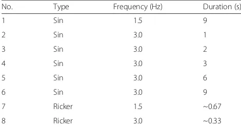
No. Type Frequency (Hz) Duration (s)

1 Sin 1.5 9

7 Ricker 1.5 ~0.67

(8)

bending processes during wave propagation. The spatial variations of wave amplitude were stronger for the 3-Hz simulation than for the 1.5-Hz simulation.

The hypocentral distance variations of the maximum amplitudes in the random inhomogeneous acoustic media (model A) are shown in Fig. 6b. To collect sufficient data, we conducted four FDM simulations using four differ-ent realizations of random media. The appardiffer-ent attenuation of maximum amplitudes was due to geometrical spreading and scattering effects. An increase in the variation of ampli-tude was observed with increasing hypocentral distance; however, the variation in amplitude was barely detectable at small hypocentral distances. As a result, we observed up to

ten-times difference between the largest and the smallestP

-wave amplitudes. The increasing variation in amplitude with increasing hypocentral distance appeared to saturate at a certain distance (~30 km) in the 3-Hz simulation.

The distribution of log-amplitudes at each hypocentral distance resembled a normal distribution (Fig. 7). This is similar to the findings of Hoshiba (2000), obtained using phase screen method simulations for plane wave propagation in 3D Gaussian-type random acoustic media. Under the first-order Rytov approximation, the log-amplitude of randomly scattered waves statistically follows a normal distribution (e.g., Andrews and Phil-lips 2005). Furthermore, our results also showed a broadening of the log-amplitude distribution with increasing frequency.

50 100 150

Y [km]

50 100 150

X [km]

1.5 Hz

50 100 150

X [km]

3.0 Hz

log

10

(P

[arb. unit]

max

)

10 10 10

P [arb. unit]

max

0 20 40 60 80 100

Hypocentral Distance [km]

1.5 Hz

10 10 10

0 20 40 60 80 100

3.0 Hz

a

b

(9)

To quantify the variation in wave amplitude, we used the

amplitude level varianceσ2

χ;as defined by Eq. (8). For

sim-plicity and practical convenience, instead of usingUin this

equation, we used the maximum amplitude for the analysis

of time-domain waveforms. The value ofσ2_χ increased with

hypocentral distance, with the increase rate differing be-tween the 1.5- and 3-Hz waves (Fig. 8). The rates of in-crease and the absolute values of the amplitude level variance were smaller for 1.5-Hz waves (no. 1 source time function). For this lower-frequency wave, the amplitude level variance monotonically increased over the whole hy-pocentral distance range. In contrast, for the 3-Hz wave (no. 6 source time function), the amplitude level variance became saturated at a distance of ~30 km, after which we observed a roughly flat data distribution at large hypocen-tral distances. The results also showed that the analytical evaluations of Eq. (13) can explain the results of the FDM simulations, with the exception of the slight underestima-tion in the 1.5-Hz wave data. We interpreted that the hypo-central distance range where the amplitude level variance of the 3-Hz wave became saturated corresponded to the strong wavefield fluctuation regime, where the weak fluctu-ation approximfluctu-ation of Eq. (13) was not appropriate.

Amplitude fluctuations: source wavelet dependence

Earthquake sources radiate non-time-harmonic waves, especially at low frequencies below the corner frequency. Thus, for the application of Eq. (13) to substantial earth-quake data, it was necessary to check the extent to which the time-harmonic wave predictions explained the amplitude level variance for non-time-harmonic waves.

We performed a numerical experiment in which the Ricker wavelet was used as non-time-harmonic wave in the FDM simulations (Fig. 9). The results of both the 1.5- and 3-Hz simulations showed no apparent differ-ences in the amplitude level variance between the two wave types in the weak wavefield fluctuation regime

σ2

χ<0:17

. However, in the strong wavefield

fluctu-ation regime, the amplitude level variance was larger for the Ricker wavelet than that for quasi-time-harmonic waves; therefore, amplitude fluctuations may depend on the duration of the source wavelet.

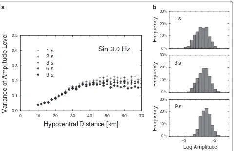
To evaluate the dependence of the duration of source time function on the amplitude level variance, we con-ducted FDM simulations using different sin waves,

which had 1, 2, 3, 6, and 9 s durations (no. 2–6 source

1.5Hz

30km

Frequency

50km

Log Amplitude

70km

3.0Hz

30km

50km

Log Amplitude

70km

0 % 10 % 20 % 30 %

(10)

time functions). The amplitude level variance in the weak wavefield fluctuation regime was very similar among the different durations of source time function (Fig. 10a); however, the values in the strong wavefield fluctuation regime increased with the decreasing dur-ation of the source time function. As discussed, the log-amplitudes for quasi-time-harmonic waves resembled a normal distribution (Fig. 7), and this characteristic was also observed for non-time-harmonic waves with shorter durations (Fig. 10b); however, the peak of the distribu-tion shifted to smaller log-amplitudes concurrently with the expansion of the left-side tail of the distribution to-ward the same side. This finding implies that increases in amplitude level variance may be due to insufficient energy supply for the constructive interference of short duration source-radiated wavelets.

Our findings showed that Eq. (13) with an adequate saturation limit may be practically effective for estimat-ing the amplitude level variance of not only time-harmonic waves, but also non-time-time-harmonic waves,

despite the slight under estimation in the strong wave-field fluctuation regime for non-time-harmonic waves.

Amplitude fluctuations: medium-type dependence

In addition to numerical analyses using random acoustic media, we conducted additional FDM numerical simula-tions using elastic random media in order to investigate the dependence of elastic parameter fluctuations on the amplitude level variance.

The hypocentral distance variation of the amplitude level variance obtained for the elastic random media was very similar to that obtained for the acoustic random media, except for small differences in absolute values (Fig. 11b). The ratio of the amplitude level variance of the acoustic random media to that of the elastic random media had a constant value ~0.8, irrespective of hypo-central distance (Fig. 11b). This indicates that amplitude variation was systematically smaller for the elastic ran-dom media than for the acoustic ranran-dom media. While the physical and quantitative interpretations of this

0.0

0 10 20 30 40 50 6 0

0 10 20 30 40 50 6

0 7 0 70

1.5 Hz

Fig. 9Hypocentral distance variations of amplitude level variance for different source time functions. Hypocentral distance variations of amplitude level variance for different source time functions using medium model A and the no. 1, 6, 7, and 8 source time functions for FDM simulations.Grey circlesshow the simulation results for the no. 1 and 6 source time functions (sin wave).Open squaresshow simulation results for the no. 7 and 8 source time functions (Ricker wavelet)

0.0

0 10 20 30 40

0 10 20 30 40 50 60 70

3.0 Hz

(11)

result remain an open question, it may allow us to apply theoretical estimation of Eq. (13) to elastic wave analysis. We compared the hypocentral distance variations of the amplitude level variance of Ricker wavelets using three random inhomogeneous media (Fig. 12): acoustic random media, elastic random media, and elastic ran-dom media without density fluctuations (models A, B, and C, respectively). When comparing the acoustic and elastic random media, we found a result similar to that seen for quasi-time-harmonic waves: the amplitude vari-ation was systematically smaller for the elastic random media than for acoustic random media, although this characteristic became obscure at large hypocentral distances (>50 km). This result was also very similar to that of the comparison between the elastic random media and the elastic random media without density fluctuations. This indicates that the main cause of the amplitude fluctuations in weak random elastic media is not density fluctuations but velocity fluctuations, im-plying that phase modulation, focusing, and defocus-ing due to complex ray-benddefocus-ing are crucial for amplitude fluctuation.

Predictions for spherical waves and plane waves

Hypocentral distance variations in the ratio of the ampli-tude level variance between spherical and plane waves

were investigated using different wavenumbers (π/4,π/2,

π, 2π, and 4πkm−1). The results for plane waves were

estimated by setting γ= 1 in Eq. (13). We assumed an

exponential-type acoustic random media with a= 1 km

and ε= 0.03 (model A). The wavenumber value πkm−1

roughly corresponded to the 3-Hz frequency in the pre-vious FDM simulations. The ratio was invariably greater than one (Fig. 13), indicating that the amplitude level variance of plane waves was always greater than that of spherical waves. The difference was especially distinct at small hypocentral distances and for high wavenumber waves, which was a reasonable result given that plane waves suffer the effects of wave propagation across a much wider inhomogeneous volume than do spherical waves. These results indicate that for analyzing ampli-tude variations of seismic waves at small hypocentral distances and in the high-frequency range, a formulation developed for spherical wave propagation is required for data analysis.

0.0 0.1 0.2 0.3 0.4 0.5

Variance of Amplitude Level

0 10 20 30 40 50 60 70

Hypocentral Distance [km]

1 s

2 s

3 s

6 s

9 s

Sin 3.0 Hz

0 %

10 % 20 % 30 %

Frequency

1 s

0 % 10 % 20 % 30 %

Frequency

3 s

0 % 10 % 20 % 30 %

Frequency

Log Amplitude

9 s

a

b

(12)

Analytical predictions and observational results

The amplitude level variance for the observed P-waves

increased with increasing hypocentral distance (Fig. 14a). The rates of increase and absolute values of the

ampli-tude level variance were smaller for 1–2-Hz waves than

those for 2–4-Hz waves. For the lower-frequency waves,

the absolute values of the amplitude level variance monotonically increased over the whole hypocentral

distance range, despite large data scatter. In contrast, for

the 2–4-Hz waves, the increases in the absolute values

of variance became saturated at a distance of ~30 km. These characteristics were successfully explained by the analytical evaluations of Eq. (13).

Despite the small data volume, the log-amplitude

dis-tribution ofP-waves observed at hypocentral distance of

70 km appeared to show a normal distribution rather than a uniform distribution (Fig. 14b). This characteristic was consistent with the results obtained by the FDM simulations (Figs. 7 and 10b); furthermore, the wider distribution for high-frequency waves was also consist-ent with the FDM simulation results.

0.0

Ratio of Variance of A. L.

0 10 20 30 40 50 60 70

Fig. 13Differences in amplitude level variance between spherical and plane waves. Ratio of amplitude level variance for spherical waves to that of plane waves for wavenumber values ofπ/4,π/2,π, 2π, and 4πkm−1_{. Stochastic parameters}_a_{= 1 km and}_ε_{= 0.03 are}

assumed. Thedotted lineindicates the region in which data are at saturation level

0 10 20 30 40 50 60 70

Fig. 12Hypocentral distance variations for amplitude level variance in different random inhomogeneous media. Hypocentral distance variations for amplitude level variance in different random inhomogeneous media using medium models A, B, and C and the no. 8 source time function for FDM simulations.Open squares denote the results for acoustic medium,open diamondsdenote the elastic medium, and theopen triangles denote the elastic (contrast density) medium

Acoustic

0 10 20 30 40 50 6 0

(13)

Focus of future analyses

The FDM simulations in this study demonstrated that variations of wave amplitude in random inhomogeneous media depend on not only the inhomogeneity of the medium but also on the duration of the source wavelet.

Thus, to use analytical Eq. (13) for the analysis of P

-waves from local and/or regional earthquakes, it is important to consider the source duration of a target earthquake, which should change by earthquake size or magnitude. In this study, in order to minimize this ef-fect, we selected similar size earthquakes for analysis. We anticipate that predictions by Eq. (13), which deals with quasi-time-harmonic waves, will be more suitable for data from large earthquakes with long source time durations. However, a detailed quantitative analysis of

earthquake-size dependence onP-wave amplitude

varia-tions will be the focus of future work.

In this study, we also restricted our focus to P-wave

analysis. Thus, applying analytical estimations using Eq. (13) to strong ground motion prediction is not straight-forward, in particular because peak ground motions

(e.g., peak ground velocity) are mainly excited by S

-waves (e.g., Atkinson and Mereu 1992). However, we be-lieve that estimations from Eq. (13) are practically useful

for the evaluation of S-wave amplitude variations in

inhomogeneous crust because the Rytov approximation has been successfully applied to the analysis of vector waves (e.g., electromagnetic wave propagation; Ishimaru 1997). From the analysis of strong motion data, Midori-kawa and Ohtake (2003) reported that the variance of peak horizontal accelerations and velocities increased with increasing hypocentral distance over a short range (<50 km), but decreased with increasing earthquake magnitude. These characteristics are consistent with

those found for P-waves in this analysis, suggesting the

applicability of our methodology to strong ground mo-tion predicmo-tion in earthquake engineering.

Conclusions

To better understand the amplitude fluctuations of high-frequency seismic waves, we carried out observational, theoretical, and numerical analyses of waves propagating in random inhomogeneous media.

Our seismic observations of theP-wave amplitudes of

small to moderately sized crustal earthquakes revealed

that the fluctuation ofP-wave amplitude increased with

increasing hypocentral distance, with up to ten-times

dif-ference between the largest and the smallestP-wave

ampli-tudes. The saturation of this phenomenon occurred at certain hypocentral distances. Furthermore, the observed

0.0

0 10 20 30 40 50 60 70

(14)

amplitude fluctuations and their rate of increase with the hypocentral distance increased with increasing frequency.

Our theoretical studies presented an analytical equa-tion for evaluating the amplitude fluctuaequa-tion of time-harmonic waves isotropically radiated by a point source and spherically propagating in acoustic von Kármán-type random media. The equation approximately explained

the characteristics of P-wave amplitude fluctuations

ob-served from local crustal earthquake as a function of frequency and hypocentral distance. Using this equation, we confirmed the differences in amplitude fluctuation between spherical and plane waves. It was verified that the amplitude fluctuations of plane waves are greater than those of spherical waves when compared at the same travel distance from source.

Our numerical analyses based on FDM simulations en-abled us to investigate the characteristics of wave propa-gation in both acoustic and elastic random media using a variety of source time functions. The results of the simulation showed that the hypocentral distance varia-tions of the amplitude fluctuavaria-tions obtained for the elastic random media were similar to those obtained for the acoustic random media, except for some differences in absolute values (i.e., the amplitude fluctuation was slightly smaller for the elastic random medium than for the acoustic random medium). We found that the values of the variance of the amplitude level in the weak wave-field fluctuation regime were very similar among the different source time function durations; however, the values in the strong wavefield fluctuation regime in-creased with decreasing duration. These results indicate that our analytical equation for amplitude fluctuations may be useful in the analysis of substantial seismic data.

Competing interests

The authors declare that they have no competing interests.

Authors_’contributions

KY carried out the theoretical consideration of amplitude fluctuations in an inhomogeneous media and drafted the manuscript. ST conducted the 3D FDM simulations and helped draft the manuscript. MK analyzed the observed seismograms of the Hi-net/F-net. All authors approved the final manuscript.

Acknowledgements

We thank two anonymous reviewers, and the editor, Takuto Maeda, for constructive comments that improved an earlier draft of this manuscript. We acknowledge the National Research Institute for Earth Science and Disaster Prevention, Japan for providing the Hi-net/F-net waveform data and the CMT solutions from the F-net. We also used the unified hypocentral catalog provided by the Japan Meteorological Agency. The FDM simulations of seismic wave propagation were conducted on the computer system of the Earthquake and Volcano Information Center at the Earthquake Research Institute, The University of Tokyo. The authors are particularly indebted to Haruo Sato and Hisashi Nakahara for valuable comments and discussions concerning wave propagation in inhomogeneous media. All figures were drawn using the Generic Mapping Tools software package developed by Wessel and Smith (1998).

Author details

1_{Department of Material System Science, Graduate School of}

Nanobioscience, Yokohama City University, 22-2, Seto, Kanazawa-ku, Yokohama 236-0027, Japan.2National Research Institute for Earth Science and Disaster Prevention, 3-1, Tennodai, Tsukuba, Ibaraki 305-0006, Japan.

Received: 17 October 2015 Accepted: 28 November 2015

References

Abramowitz M, Stegun IA (1964) Handbook of mathematical functions: with formulas, graphs, and mathematical tables. U. S. Govt. Printing Office, Washington

Aki K, Richards P (2002) Quantitative seismology (2nd edition). University Science Books, Freeman, San Francisco

Anderson JG, Uchiyama Y (2011) A methodology to improve ground-motion prediction equations by including path corrections. Bull Seismol Soc Am 101(4):1822_–1846. doi:10.1785/0120090359

Andrews LC, Phillips RL (2005) Laser beam propagation through random media, 2nd edn. SPIE Publications, Washington

Atkinson GM (2006) Single-station sigma. Bull Seismol Soc Am 96(2):446–455. doi:10.1785/0120050137

Atkinson GM, Mereu RF (1992) The shape of ground motion attenuation curves in southeastern Canada. Bull Seismol Soc Am 82(5):2014–2031

Birch AF (1961) The velocity of compressional waves in rocks to 10 kilobars, part 2. J Geophys Res 66:2199_–2224. doi:10.1029/JZ065i004p01083

Brillinger DR, Preisler HK (1984) An exploratory analysis of the Joyner-Boore attenuation data. Bull Seismol Soc Am 74(4):1441–1450

Chen YH, Tsai CCP (2002) A new method for estimation of the attenuation relationship with variance components. Bull Seismol Soc Am 92(5):1984_–1991. doi:10.1785/0120010205

Douglas J (2003) Earthquake ground motion estimation using strong motion records: a review of equations for the estimation of peak ground acceleration and response spectral ordinates. Earth Sci Rev 61:43_–104. doi:10.1016/S0012-8252(02)00112-5

Flatté SM, Wu RS (1988) Small-scale structure in the lithosphere and asthenosphere deduced from arrival time and amplitude fluctuations at NORSAR. J Geophys Res 93:6601_–6614. doi:10.1029/JB093iB06p06601 Fukuyama E, Ishida M, Dreger DS, Kawai H (1998) Automated seismic moment

tensor determination by using on-line broadband seismic waveforms. Zisin 51:149–156 (in Japanese with English abstract)

Furumura T, Chen L (2004) Large scale parallel simulation and visualization of 3D seismic wavefield using Earth simulator. Comput Model Eng Sci 6:153–168 Hoshiba M (2000) Large fluctuation of wave amplitude produced by small

fluctuation of velocity structure. Phys Earth Planetary Int 120(3):201–217. doi:10.1016/S0031-9201(99)00165-X

Ishimaru A (1997) Wave propagation and scattering in random media. IEEE Press and Oxford University Press, ISBN: 078034717X.

Kobayashi M, Takemura S, Yoshimoto K (2015) Frequency and distance changes in the apparent P-wave radiation pattern: effects of seismic wave scattering in the crust inferred from dense seismic observations and numerical simulations. Geophys J Int 202:1895–1907. doi:10.1093/gji/ggv263 Lin PS, Chiou B, Abrahamson N, Walling M, Lee CT, Cheng CT (2011) Repeatable

source, site, and path effects on the standard deviation for empirical ground-motion prediction models. Bull Seismol Soc Am 101(5):2281–2295. doi:10.1785/0120090312

Mavroeidis GP, Papageorgiou AS (2003) A mathematical representation of near-fault ground motions. Bull Seismol Soc Am 93(3):1099_–1131. doi:10.1785/0120020100

Midorikawa S, Ohtake Y (2003) Empirical analysis of variance of ground motion intensity in attenuation relationships. J Japan Assoc Earthquake Eng 3(1):59_–70, http://doi.org/10.5610/jaee.3.59 (in Japanese with English abstract) Müller TM, Shapiro SA (2003) Amplitude fluctuations due to diffraction and

refraction in anisotropic random media: implications for seismic scattering attenuation estimates. Geophys J Int 155(1):139–148. doi:10.1046/j.1365-246X. 2003.02020.x

Nikolaev A V (1975) The seismics of heterogeneous and turbid media (Engl. trans. by Hardin R), Israel program for science translations, Jerusalem

(15)

Ripperger J, Mai PM, Ampuero JP (2008) Variability of near-field ground motion from dynamic earthquake rupture simulations. Bull Seismol Soc Am 98(3): 1207–1228. doi:10.1785/0120070076

Ritter JRR, Shapiro SA, Schechinger B (1998) Scattering parameters of the lithosphere below the Massif Central, France, from teleseismic wavefield records. Geophys J Int 134(1):187_–198. doi:10.1046/j.1365-246x.1998.00562.x Rytov SM, Kravtsov YA, Tatarskii VI (1989) Principles of statistical radiophysics,

Vol. 4, Wave propagation through random media. Springer-Verlag, Berlin Sato H, Fehler MC, Maeda T (2012) Seismic wave propagation and scattering in the heterogeneous earth: the second edition, 1_–494. Springer Verlag, Berlin Hidelberg

Shapiro SA, Kneib G (1993) Seismic attenuation by scattering: theory and numerical results. Geophys J Int 114:373–391. doi:10.1111/j.1365-246X.1993. tb03925.x

Si H, Midorikawa S (1999) New attenuation relationships for peak ground acceleration and velocity considering effects of fault type and site condition. J Struct Constr Eng AIJ 523:63–70 (in Japanese with English abstract) Strasser FO, Abrahamson NA, Bommer JJ (2009) Sigma: issues, insights, and

challenges. Seismol Res Lett 80:40–56. doi:10.1785/gssrl.80.1.40 Takemura S, Furumura T, Maeda T (2015) Scattering of high-frequency seismic

waves caused by irregular surface topography and small-scale velocity inhomogeneity. Geophys J Int 201:459_–474. doi:10.1093/gji/ggv038 Uscinski BJ (1977) Elements of wave propagation in random media. McGraw-Hill,

New York

Wessel P, Smith WHF (1998) New improved version of generic mapping tools released. EOS Trans Amer Geophys Union 79(47):579. doi:10.1029/98EO00426 Yoshimoto K, Takemura S (2014) A study on the predominant period of

long-period ground motions in the Kanto Basin, Japan. Earth Planets Space 66:100. doi:10.1186/1880-5981-66-100

Yoshimoto K, Sato H, Ohtake M (1993) Frequency-dependent attenuation of P and S waves in the Kanto area, Japan, based on the coda-normalization method. Geophys J Int 114:165–174. doi:10.1111/j.1365-246X.1993.tb01476.x