R E S E A R C H
Open Access
Unified commutation-pruning technique
for efficient computation of composite
DFTs
David E. Castro-Palazuelos
1,2*, Modesto Gpe. Medina-Melendrez
1, Deni L. Torres-Roman
2and Yuriy V. Shkvarko
2Abstract
An efficient computation of a composite length discrete Fourier transform (DFT), as well as a fast Fourier transform (FFT) of both time and space data sequences in uncertain (non-sparse or sparse) computational scenarios, requires specific processing algorithms. Traditional algorithms typically employ some pruning methods without any commutations, which prevents them from attaining the potential computational efficiency. In this paper, we propose an alternative unified approach with automatic commutations between three computational modalities aimed at efficient computations of the pruned DFTs adapted for variable composite lengths of the non-sparse input-output data. The first modality is an implementation of the direct computation of a composite length DFT, the second one employs the second-order recursive filtering method, and the third one performs the new pruned decomposed transform. The pruned decomposed transform algorithm performs the decimation in time or space (DIT) data acquisition domain and, then, decimation in frequency (DIF). The unified combination of these three algorithms is addressed as the DFTCOMMtechnique. Based on the treatment of the combinational-type hypotheses
testing optimization problem of preferable allocations between all feasible commuting-pruning modalities, we have found the global optimal solution to the pruning problem that always requires a fewer or, at most, the same number of arithmetic operations than other feasible modalities. The DFTCOMMmethod outperforms the existing
competing pruning techniques in the sense of attainable savings in the number of required arithmetic operations. It requires fewer or at most the same number of arithmetic operations for its execution than any other of the competing pruning methods reported in the literature. Finally, we provide the comparison of the DFTCOMMwith
the recently developed sparse fast Fourier transform (SFFT) algorithmic family. We feature that, in the sensing scenarios with sparse/non-sparse data Fourier spectrum, the DFTCOMMtechnique manifests robustness against such
model uncertainties in the sense of insensitivity for sparsity/non-sparsity restrictions and the variability of the operating parameters.
Keywords:Composite length discrete Fourier transform, Decimation, Decomposition, Fast Fourier transform, Pruning
1 Introduction
1.1 Motivation
Many signal processing applications require computation of the so-called pruned discrete Fourier transform (DFT), i.e., an efficient alternative to compute the required DFT when the input sequence and/or the required output se-quences are smaller than the length of the full DFT (a full
DFT means that all the output components are to be computed, and all the input elements are used to compute the transform); in the literature those are referred to as pruned fast Fourier transforms (FFTs) or pruned DFTs [1]. Common practical examples relate to, e.g., the least mean squared (LMS) optimal DFT-based pruned signal filtering [2], and the complexity-reduced computational imple-mentation of the orthogonal frequency division multiplex-ing systems [3]. Another practical example relates to efficient implementation of the matched spatial filtering (MSF) algorithm for performing the range and azimuth data compression in unfocused of fractionally focused
* Correspondence:[email protected]
1
Department of Electrical-Electronic Engineering, Culiacan Technological Institute, Ave. Juan de Dios Batiz S/N, Col. Guadalupe, C.P. 80220 Culiacan, Sinaloa, Mexico
2Telecommunications Group, CINVESTAV-IPN Campus Guadalajara, Ave. del
Bosque 1145, Col. el Bajio, C.P. 45019 Zapopan, Jalisco, Mexico
synthetic aperture radar (SAR) system that both employ the pruned DFT-based MSF processing of the trajectory data signals performed in a factorized fashion in the so-called slow time and fast time data acquisition scales [4–6]. Other examples relate to DFT-based analysis of remote sensing (RS) data acquired with a variety of sen-sor systems, ranging from seismology [7] to multispec-tral radiometry [8]. Other authors as Zhu et al. in [9] proposed an algorithm for performing SAR polar for-mat re-gridding interpolation suited for the logic-in-memory paradigm (hardware/architecture solution) and to provide the necessary design automation tool chain to implement their proposed algorithm (e.g., FFTs for image formation) in advanced silicon technology. It is important to note that a majority of real-world RS data acquisition and processing problems can be qualified as sensing in harsh environments [4–8, 10, 11] in the sense of intrinsic problem model uncertainties peculiar for such RS modalities. In a context of pruned DFTs, realistic harsh sensing scenarios are characterized by the uncertainties attributed to zero-padded input data acquisition modes with variable composite length win-dowing of the input and/or output Fourier transform sequences, in general cases, with non-sparse Fourier spectra [10–12]. Those specifics motivate the develop-ment of efficient pruned DFT/FFT techniques particu-larly adapted for computational implementation with uncertain data acquired in harsh sensing scenarios.
1.2 Related work
Traditional DFT algorithms adapted for such uncertain scenarios typically employ some pruning methods with-out any commutations, which prevent them from attain-ing the potential computational efficiency. Most of the proposals reported in the literature are based on con-struction of pruning modalities of specific FFT-related algorithms. Some of them prune the input of a specific FFT algorithm, others prune the output, and just a few can prune the input and output (input-output) at the same time. Markel in [1], and Skinner in [13], proposed the input pruning methods based on a radix-2 FFTs, while Yuan et al., in [14], proposed an input pruning of a split-radix FFT. The approaches of Bouguezel et al. [15] and Fan et al. [16] are applicable for output pruning a radix-2 FFTs, while the Xu’s et al. [3] proposal suggests pruning the output of a split-radix FFT. In addition, Sreenivas et al., in [17], Roche, in [18], and Wang et al., in [19], developed the methods for pruning the input-output at the same time. The first one is based on a radix-2 FFT, the second one employs the split-radix FFT, and the third one performs the mixed-radix FFT, re-spectively. A majority of those methods are applicable only for computing DFTs with the length of a power of
two that drastically restricts their applicability to general uncertain sensing scenarios.
On the other hand, a family of novel so-called sparse FFT (SFFT) algorithms adapted to computing the FFTs, when only a few Fourier spectrum coefficients of the input signal are different from zero (few largest coeffi-cients of the Fourier transform spectrum), has been de-veloped recently [20, 21]. The celebrated SFFT-related algorithms, so-called SFFTv1 and SFFTv2, were reported by Hassanieh et al., in [20]. Later, in [21], the improved SFFT-related versions, addressed as SFFTv3 and SFFTv4, were reported. Another algorithm that considers the Fourier spectrum sparsity restrictions is the so-called FADFT-2 reported and implemented in the AAFFT library [22]. However, the SFFT-related algorithms significantly outperform the AAFFT as it was corroborated in [20].
It is worthwhile to mention that the SFFT-related techniques are applicableonlyfor the sparse sensing sce-narios; e.g., referring to [20, 21], the authors exemplified the sparsity level by imposing the restriction that up to 89 % of the Fourier coefficients are zeroes or negligible, thus can be discarded. Such a restriction could be valid in a variety of data compressing applications, e.g., com-pression and recovery of video data not degraded by noise and/or imaging system instrumental function [20]. Nevertheless, the restriction on such sparsity is not valid for many real-world operational scenarios, e.g., processing of the RS data acquired in harsh sensing environments [4–8, 10–12]. For example, in SAR imaging of non-homogeneous scenes, e.g., urban areas, non-uniformly textured zones, etc., a majority of the Fourier transform coefficients should be considered for feature-enhanced MSF-based imaging [5, 6]; thus, an 89 % of sparsity level restriction is never a feasible model assumption.
In this paper, we are interested in developing the pruned DFT (DFTs of highly composite length) algo-rithms applicable for near-real-time signal processing and analysis in uncertain sensing scenarios (i.e., with non-guaranteed sparsity of the data Fourier spectra); that is why the family of the SFFT-related techniques is beyond our detailed study here. Nevertheless, for the purpose of generality, in Section 4, we perform compara-tive analysis of our developed methods with the SFFT under the same conditions and constraints for different combinations of the specified processing/operational parameters.
obtain a composite structure that is capable to prune the input and/or output of a general decomposed transform at the same time. It was demonstrated, in [24], that such a computational structure could be as efficient as the one based on specific FFT algorithms [15–17]. In [24], a new methodology for decomposition over a composite length DFT has been proposed as a modification of the Soren-sen’s approach [23]. Furthermore, the [24] suggests, first, to perform decimation in frequency (DIF) and, second, a decimation in time (DIT). For processing of spatial data, the corresponding decimation in the space domain should be performed similarly to the DIT operation for time data processing. To avoid misunderstandings, in the rest of the paper, we will use the same abbreviation (DIT) for both processing models and consider the time data process-ing as a principal model. Nevertheless, all developments are directly transferable for the space data processing scenario.
Hence, the three basic stages to compute the compos-ite length DFTs of non-sparse data encompass the input, the intermediate, and the output stages. The decom-posed transform is then pruned by eliminating, from the input and output stages, additions and multiplications by zero, multiplications by one, and all other computa-tions not needed to obtain the required Fourier transform coefficients. In [24], such the multistage decomposed and pruned transform is referred to as FFTDIF−DIT−TD (here, that method is referred as DFTDIF−DIT−Pr). Nevertheless, both methods addressed in [23, 24] do not achieve the lowest attainable number of the required arithmetic oper-ations. A possible alternative for computing few Fourier coefficients from few input elements (all non-zero, thus non-sparse) can be addressed based on the application of the second-order Goertzel algorithm [23] modified to accept the input elements in a reverse order.
1.3 Novel contributions
The main contribution of this paper consists in the de-velopment of a new alternative method for efficient computing of a composite length DFT, when the input sequence and/or the required output sequence are smaller than the length of the full transform. Our pro-posal guarantees the same or smaller number of arith-metic operations in comparison with the competing methods in the literature. Moreover, it manifests robust-ness against sparsity/non-sparsity restrictions and the variability of the operating parameters as detailed in Sections 3 and 4.
The innovative idea is to automatically commute among three modalities to implement the DFT: the direct method, the recursive method, and the pruned decomposed transform. Thus, our new proposed com-posite approach unifies the decomposition of the DFT with its pruning. First, we develop an alternative
technique to compute the pruned decomposed trans-form, in which the DIT is performed at the first stage followed by the DIF. We address this method as DFTDIT−DIF−Pr. An analysis of the two alternatives (DFTDIT−DIF−Pr and DFTDIF−DIT−Pr) verifies that the DFTDIT−DIF−Prrequires a smaller or as maximum equal number of arithmetic operations compared with the DFTDIF−DIT−Pr, so the use of the DFTDIT−DIF−Pr is strongly recommended when the decomposed and pruned transforms are required. Next, we demonstrate that our proposal requires a lower number of arith-metic operations than any of the pruning-based com-peting methods [3, 14, 23, 24]. Further, we demonstrate that both decomposed transforms (DFTDIF−DIT−Pr and DFTDIT−DIF−Pr) can be obtained from a general decom-position methodology. Also, it manifests the robustness in sparse and non-sparse sensing scenarios (i.e., oper-ability for an arbitrary number of consecutive input ele-ments (Li), the number of consecutive outputs that should be computed (Lo), and the length of the full transform (N)) in contrast to the recently developed most prominent SFFT family-related methods [20, 21] operable in sparse scenarios only.
It is noteworthy to mention that in the majority of practical computational scenarios, significant savings in the number of arithmetic operations with the proposed technique are achieved, e.g., in Section 4.1, the DFTCOMM technique compared with split-radix FFT (SRFFT) algorithm produces savings of 42 to 92 %.
The rest of the paper is organized as follows: in Sec-tion 2, the general decomposiSec-tion transform methodology is described and explained. An analysis of all feasible transform decomposition methods is presented next in Section 3 followed by the combinational hypotheses test-ing optimization-based selection of the best decompos-ition transform permutation modality that yields the unified commutation-pruning DFTCOMM technique. In Section 4, comparisons among the developed unified commutation-pruning technique and other competing al-gorithms in the sense of savings in the number of required arithmetic operations are presented and featured. Also, the proposed DFTCOMM method is compared in detail with the most prominent competing SFFT-related algo-rithms in the context of computing the DFTs in both sparse and non-sparse (harsh) sensing scenarios for differ-ent values of the operational parameters (Li, Lo, andN). Concluding remarks in Section 5 summarize the study. The Appendix provides a pseudo-code for implementing the proposed method.
2 DFT transform decomposition
X kð Þ ¼X Let us defineLias the number of consecutive input ele-ments different from zero andLoas the number of con-secutive outputs that should be computed. If N is a composite number formed by multiplications of many integer factors, the DFTN can be decomposed into smaller DFTs. In particular, the DFTN can be decom-posed into three stages of DFTs (an input stage, an inter-mediate stage, and an output stage) in order to avoid the arithmetic operations involving zeros, multiplications by one, and the operations not required to compute the final outputs. Here beneath, we briefly describe such feasible decompositions. Assuming that there are two in-teger factors,Dipand Dop, ofNsuch thatN/DipDop≡P is an integer, the indexesnandkcan be re-expressed as
n¼n1þDopn2þ
Substituting n and k in (1) by (2), (3), the original DFTNis decomposed into
X k1þDipk2þ
Here, it is assumed that Dip and Dop are chosen in such a way that N/Dip≥Li and N/Dop≈Lo. Thus, index
The computation of (5) is more efficient than the direct computation of the DFTN since the complex arithmetic operations dependent onn3have been pruned. The com-plex exponential in (5) can next be grouped in different ways, resulting in different structures for the pruned decomposed transform. The methodology of [24] suggests expressing the pruned decomposed transform as
X k1þDipk2þ
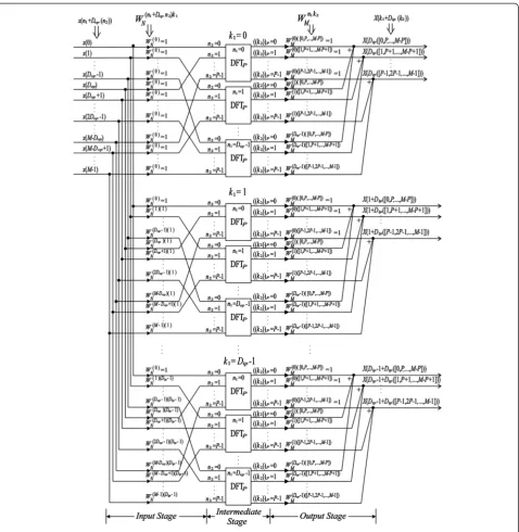
The pruned decomposed transform of (6) can be inter-preted as follows: first, apply DIF to the DFTNwithDipas a decomposition factor, then, DIT to the resulting DFTs withDop as a decomposition factor and, finally, perform the pruning. In [24], the pruned decomposed transform of (6) was addressed as an FFTDIF−DIT−TD modality, that in our notations, we refer to as DFTDIF−DIT−Pr. A
computa-tional diagram of such technique (6) is presented in Fig. 1. An alternative grouping of the complex exponentials in (5) yields
Dop as a decomposition factor and, then, application of DIF to the resulting DFTs with Dipas a decomposition factor.
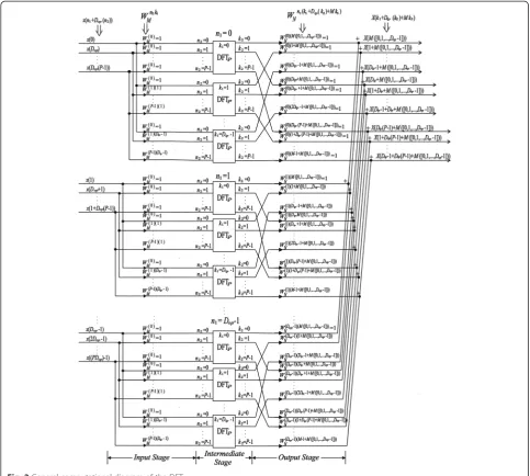
Hence, we refer to the pruned decomposed transform of (7) as a DFTDIT−DIF−Prmodality. A computational dia-gram of such the technique (7) is presented in Fig. 2.
The DFTDIT−DIF−Prinvolves three processing stages: an input stage (computation of y(n1,n2, k1)), an intermedi-ate stage (computation ofDipDopDFTs of lengthP), and an output stage (computation of the complex multiplica-tions and addimultiplica-tions dependent on indexn1).
3 Proposed method
Our method employs three different alternatives to com-pute the DFTN: a direct method, a recursive method, and/ or a pruned decomposed transform. Admissible permuta-tions/allocations of all feasible decomposition-pruning modalities compose all possible hypotheses regarding the feasible alternative schemes for computing the composite DFTs.
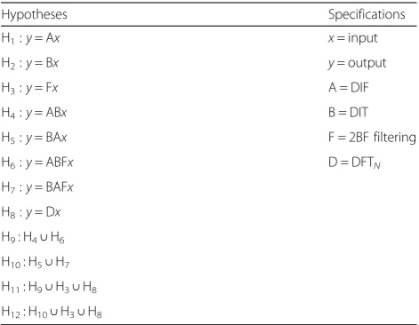
problem of selection of an optimal computing-pruning implementation structure can be recast as a hypotheses testing task. All feasible hypotheses relate to formal im-plementation structures specified in Table 1. Four of them prescribe cascade computational implementation involving cascade combinations of structures (hypoth-eses H4,…, H7), while four others (hypotheses H9,…, H12) prescribe combinational unions of the previous hy-potheses. It is important to remark that (1), (6), and (7) are the mathematical definitions of H8, H4, and H5, re-spectively. Hence, the decision-making process that is a selection from those feasible operational prescriptions cannot be formalized as an optimization strategy for minimization of some cost function subject to relevant re-strictions/constraints specified in a closed analytical form. Thus, due to the composite combinations (hypotheses
force search over complete hypotheses list specified in Table 1.
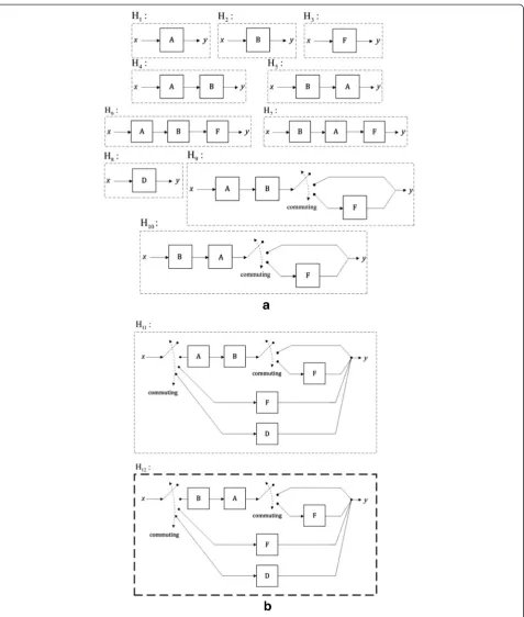
Sorensen et al. [23] sketched how to prune the input and output of DFTs using independent allocations listed in Table 1 as H1, H2, and H3 and featured in Fig. 3a. However, the authors of [23] concluded that their prun-ing method is less efficient than other prunprun-ing methods in the cases when both the number of input and output elements are bounded. They recommended turning to the method proposed by Sreenivas et al., in [17], i.e., to prune the input and output of a power of two length FFTs. Furthermore, an efficient input-output pruning method for a power of two length FFTs was proposed by Roche in [18].
Later, a more efficient input-output pruning method for composite length DFTs was developed in [24]. Such commuting between H4∪H6 leads to hypothesis H9 as featured in Fig. 3a. In [24], such a technique was con-structed as a modification of the transform decompos-ition proposed originally by Sorensen et al., in [23], but with extra capability to perform the input-output prun-ing at the same time. Additionally, the computation of each final output employs a commutation between a direct method and the 2BF filtering algorithm, i.e., the 2BF-filtering algorithm is an efficient method for com-puting a subset of final outputs from their decompos-ition transform [23, 24].
In our study, two additional feasible hypotheses are devised to perform unified commutation-pruning tech-niques for efficient computations of composite length DFTs (hypotheses H11 and H12) as reported in Fig. 3b. Therefore, our proposal relates to an adaptive commut-ing between feasible implementation structures specified by the union of hypotheses H10∪H3∪H8 that is in-cluded in Table 1 as an alternative composite hypothesis
H12. A comparison of computational complexities related to implementation of the competing computational struc-tures formalized by hypotheses H9and H10 (in the num-ber of required arithmetical operations) is reported in Table 2. Also, the relevant comparisons between two other feasible structures specified by hypotheses H11 and H12 (referred here as DFTCOMM−DIF−DIT−Prand DFTCOMM−DIT−
DIF−Pr, respectively), are reported in Tables 2 and 3 and Figs. 5a–f (in the sense of the number of required arith-metic operations).
The selection of proper permutation/allocation struc-ture directly relates to the considered above problem of selection of an optimal commutation-pruning implemen-tation structure casted and treated as a combinational hypotheses testing task. All feasible hypotheses fHhg12h¼1 relate to formal implementation structures specified in Table 1. Now, we are ready to find the best permutation/ allocation structure in the sense of the imposed quality measure (in our case in the sense of the lowest possible number of required arithmetical operations).
3.1 Analysis of the hypotheses
Let us analyze, first, the pruned decomposed transform and deduce whether the direct or recursive method would be preferable. The total number of arithmetic op-erations (OPERtot) required by the DFTDIF−DIT−Pr and the DFTDIT−DIF−Prdepends on the number of operations needed to be performed to implement the input stage (OPERinput), the output stage (OPERoutput), and the intermediate stage (DipDopOPERDFTP), correspondingly. Thus, one could express OPERtot of both pruned decomposed transforms as
OPERtot¼OPERinputþDipDopOPERDFTPþOPERoutput: ð8Þ
According to (8), OPERtot depends on Li, Lo, N, Dip, Dop, and the algorithm employed to implement theDip -DopDFTPblocks (OPERDFTP).
At the input and output stages, there are multiplica-tions by one, so those multiplicamultiplica-tions are avoided at all in our approach. Also, the multiplications by one at the input stage are also avoided depending on whether DFTDIF−DIT−Pr or DFTDIT−DIF−Pr was executed in the particular employed pruned decomposed transform modality.
If the DFTDIF−DIT−Pr modality is employed (see the general diagram in Fig. 1), then:
At the input stage, the multiplications by one are excluded whenn1=n2= 0 andk1= 0.
Furthermore, the multiplications by one at the output stage are also avoided whenn1= 0 ork2= 0.
Table 1Complete list of hypothesesfHhg12h¼1regarding feasible
Therefore, the DFTDIF−DIT−Prmodality always requires fewer complex multiplications to compute the output stage than the DFTDIT-DIF-Prmodality (this is reported in Tables 2 and 3).
On the other hand, if the DFTDIT-DIF-Pr modality is used (see Fig. 2), then:
At the input stage, the multiplications by one are excluded whenn2= 0 ork1= 0.
Also, at the output stage, the multiplications by one are avoided whenk1=k2= 0 orn1= 0.
Therefore, the DFTDIT-DIF-Pr modality always requires fewer complex multiplications at the input stage than the DFTDIF−DIT−Prmodality (as it is corroborated in the analysis reported in Tables 2 and 3).
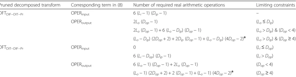
The output stage of both pruned decomposed trans-form modalities can be computed by the direct addition of complex multiplications or a kind of recursive algo-rithm as those proposed in [23] (referred to as the 2BF filtering method), which reduces the number of required multiplications by about half. The number of arithmetic multiplications required by the output stage of the DFTDIF−DIT−Pralgorithm is equal to 4 (Lo−Dip) (Dop−1) when (Lo>Dip) and (Dop< 4). Next, the number of arith-metic multiplications is equal to (Lo−Dip) (2Dop+ 2) when (Lo>Dip) and (Dop≥4). Thus, the 2BF filtering al-gorithm can be effectively used to compute the output stage.
On the other hand, the number of arithmetic multi-plications required to compute the output stage of the DFTDIT-DIF-Pr algorithm is equal to 4(Lo−1) (Dop−1) when (Dop< 4); and the number of arithmetic
multiplications is equal to (Lo−1) (2Dop+ 2) when (Dop≥4). Thus, the 2BF filtering algorithm can also be effectively employed to compute the output stage.
In [23], it was proven that the 2BF filtering method is more efficient than the direct addition of complex multi-plications when the number of input elements is larger than 4 (when the number of input elements is equal to 4, both methods manifest the same operational complex-ity performances). The output stages of both pruned decomposed transforms have the same structures, so same sort of commutations is required to efficiently compute the output stage of the DFTDIT−DIF−Pr. The ex-pressions for OPERinput and OPERouput for the DFTDIF−
DIT−Prand the DFTDIT−DIF−Prare listed in Table 2, where it is implicitly assumed that each complex multiplication requires six arithmetic operations (four real multipli-cations and two real additions), and each complex addition requires two arithmetic operations (two real additions).
The performances of the pruned decomposed trans-forms depend on the decomposition factors, Dip and Dop. A simple analysis can be carried out to deduce which decomposition factors are preferable to be used. Our unified commutation-pruning method performs the decomposition of the DFTNinto three stages of smaller dimension DFTs and pruning part of those inputs that are equal to zero and/or part of those outputs that are not needed to compute the final Fourier coefficients.
Thus, the decomposed transform algorithm always se-lects a pair (Dip, Dop) for which the largest DFTs could be successfully pruned, or equivalently, a pair (Dip, Dop) for which the intermediate stage results in the smallest dimension DFTs.
Table 2Total number of arithmetic operations required to compute the input and output stages of DFTDIF−DIT−Prand DFTDIT−DIF−Pr
Pruned decomposed transform Corresponding term in (8) Number of required real arithmetic operations Limiting constraints
DFTDIF−DIT−Pr OPERinput 6 (Li−1) (Dip−1) –
Number of required operations when the 2BF filtering method is employed [23,24]
Table 3Total number of arithmetic operations required to compute the input and output stages of DFTCOMM−DIF−DIT−Prand
DFTCOMM−DIT−DIF−Prmodalities
Method to compute the DFTN Number of arithmetic operations Limiting conditions
Direct method 6 (Lo−1) (Li−1) + 2Lo(Li−1) ((Li≤Dop)|(Lo≤Dip)) & (Li< 4)
2BF filtering method (Lo−1) (2Li+ 2) + 2 (Li−1) + (Lo−1) (4Li−2) ((Li≤Dop)|(Lo≤Dip)) & (Li≥4)
The DFTs of the intermediate stage have a size of N/ DipDop≡P, so Dip andDopshould be chosen as large as possible. Furthermore, the values for the decomposition factors should satisfy the boundN/Dip≥Li(where,N/Dip must be close to but higher thanLi) andN/Dop≈Lo, as it was considered in the derivation of (5). Hence, the pair of decomposition factors (Dip, Dop) closest to (N/Li, N/ Lo) that satisfy Dip≤N/Li are used by the decomposed transform algorithm, according to the proximity evalu-ated by its Euclidean distance.
Let us now consider the cases when the number of in-put elements (Li) or the number of the required Fourier coefficients (Lo) is too small. In these cases, for the both modalities, the general diagrams presented in Figs. 2 and 1 clarify the following features of the DFTDIT−DIF−Prand the DFTDIF−DIT−Pralgorithms, respectively.
IfLi≤Dop, at most one input of each DFTP(i.e., the
first one) in the intermediate stage would be applied; therefore, theirPoutputs would be replicas of that single input.
ForLo≤Dip, only the first output of each DFTP(this
corresponds to a simple addition of the input elements) is required to compute the final Fourier coefficients.
Thus, inefficient implementations of the DFTPs yield the inequality-type constraints Li≤Dop or Lo≤Dip. In these cases, our method commutes to efficiently perform the direct computation of the DFTN or an efficient re-cursive alternative (via performing the 2BF filtering technique).
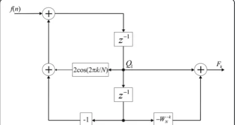
Sorensen et al., in [23], proposed a method to compute a subset of the output components of their proposed specific DFT decomposition; this algorithm was referred to as a 2BF filtering method. The 2BF filtering method [23] was derived as a modification of the previously ad-dressed Goertzel algorithm [25]. The 2BF filtering method takes advantages of the periodicity and the shifted cyclic convolution shape between the input se-quence and theWnkN ¼e−jð2π=NÞknfactor.
The transfer function H(z) of a system that performs the 2BF filtering method is given by the equation
H zð Þ ¼ z−1 1−z−1W−Nk
1−2 cos 2πk
N z−1þz−2
ð9Þ
The corresponding algorithmic diagram of the second-order 2BF method is presented in Fig. 4. Thus, (9) is the mathematical definition of H3.
The poles of the system transfer function (the roots of the polynomial in the denominator of H(z)) have to be evaluated L times (n= 0, 1, 2,…, L−1), while the zeros of the system transfer function (the roots of the
numerator of H(z)) only once. Here, L represents the number of consecutive non-zero input elements of the 2BF filter; i.e., in the opposite case, it represents the number of consecutive non-zero output components of the employed pruned decomposed transform modality (DFTDIF−DIT−Pror DFTDIT−DIF−Pr).
The computation of each pole of (9) requires two arithmetic multiplications (two real multiplications) and two arithmetic additions (two real additions). Further-more, the computation of the zeros of (9) requires four arithmetic multiplications and four arithmetic additions only.
TheQ1node in Fig. 4 is initialized withf(L−1); there-fore, the computation starts fromn=L−2. When n= 0, the complex addition of the input is only required; then, the zero is computed after such a delay. Such computa-tional organization saves two arithmetic multiplications and six arithmetic additions for finding of each required output component.
The 2BF filtering method employed to compute the output components required by the pruned decomposed transform performed by the DFTCOMM−DIF−DIT−Pr or the DFTCOMM−DIT−DIF−Pr algorithm can be featured as the following multistage procedure:
The structure of the DFTDIF−DIT−PrcontainsDipsets
ofDopDFTPs from which the final outputs are
computed (see the general diagram in Fig.1).
The DFTCOMM−DIF−DIT−Pralgorithm employs the 2BF
filtering method to implement the output stage of DFTDIF−DIT−PrwithL=Lo, if ( (Li>Dop) & (Lo>Dip) )
& ( (Lo>Dip)&(Dop≥4) ) (as featured in Tables2and 3). Here, the required arithmetic operations are specified as follows: the number of arithmetic multiplications are equal toNumArithMult2BF=
(Lo−Dip)(2Dop+ 2) and the number of arithmetic
additions are equal toNumArithAdd2BF= 2Dip
(Dop−1) + (Lo−Dip)(4Dop−2).
Furthermore, the DFTCOMM−DIF−DIT−Pralgorithm
employs the 2BF filtering method exclusively with
L=Li, if ( (Li≤Dop) | (Lo≤Dip) ) & (Li≥4) (as
featured in Table3) to compute the required Fourier coefficients. Here, the required arithmetic operations are specified as follows:NumArithMult2BF= (Lo−
1)(2Li+ 2) andNumArithAdd2BF= 2(Li−1) + (Lo−
1)(4Li−2).
In contrast, the DFTCOMM-DIT-DIF-Pr algorithm differs from the abovementioned in the following features:
The structure of the DFTDIT-DIF-PrcontainsDopsets
ofDipDFTPs from which the final outputs are
computed (as featured in Fig.2).
The DFTCOMM-DIT-DIF-Pralgorithm employs the 2BF
filtering method to implement the output stage of DFTDIT-DIF-PrwithL=Lo, if ( (Li>Dop) & (Lo>Dip) )
& (Dop≥4), (as featured in Tables2and3). Here,
the required arithmetic operations are specified as follows:NumArithMult2BF= (Lo−1)(2Dop+ 2), and
NumArithAdd2BF= 2 (Dop−1) + (Lo−1)(4Dop−2).
On the other hand, the DFTCOMM-DIT-DIF-Pr
algorithm employs the 2BF filtering method exclusively withL=Li, if ( (Li≤Dop) | (Lo≤Dip) ) &
(Li≥4) (as reported in Table3) to compute the
required Fourier coefficients. Here, the required arithmetic operations are specified as follows:
NumArithMult2BF= (Lo−1)(2Li+ 2) and
NumArithAdd2BF= 2(Li−1) + (Lo−1)(4Li−2).
The computation of each input and/or output element in both cases detailed above is executed according to the diagram presented in Fig. 4. In closing, we note that the pseudo-code presented in the Appendix (see Fig. 9) con-tains all scripts needed to compute each Fourier coeffi-cient employing the 2BF filtering method.
Note once again that the 2BF filtering method has to be employed ifLiis larger or equal to 4, in which case, it manifests a higher efficiency than the direct method for computing the DFTN in (1). The total number of arith-metic operations required by our proposed method is re-ported in Table 3.
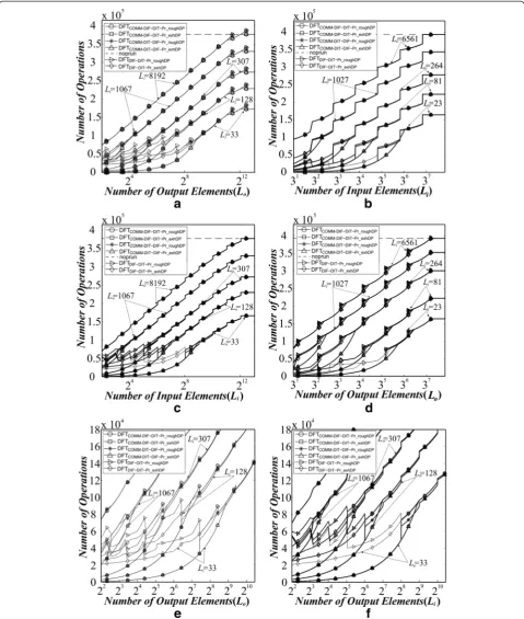
3.2 Selection of the permutation/allocation structure In Fig. 5, the total number of required arithmetic opera-tions to compute the DFTDIF−DIT−Pr from [24] (H9), DFTCOMM−DIF−DIT−Pr (H11), and DFTCOMM−DIT−DIF−Pr (H12) modalities are plotted for different values ofLiand Lo for the test examples withN= 8192 andN= 6561 (It is assumed that the DFTPs are implemented employing the split-radix algorithm from [26] for N= 8192 and employing the radix-3 algorithm from [27] for N= 6561.) All the competing alternatives corresponding to three feasible arrangements (H9, H11, and H12) in the considered permutation/allocation structure are featured
in Fig. 5. The DFTDIF−DIT−Pror the DFTDIT−DIF−Prcould be used to implement the pruned decomposed trans-form in the DFTCOMM−DIF−DIT−Pr and DFTCOMM−DIT−
DIF−Pr techniques. Here, the Dip and Dop values are the pair specified by the rough selection method (the prox-imity evaluated by its Euclidean distance is referred as roughDP) and those obtained by an exhaustive search method (the total numbers of operations required to im-plement the DFTDIF−DIT−Pr and the DFTDIT−DIF−Pr were evaluated for each possible pair of (Dip, Dop), and, then, the pair (Dip, Dop) with the best performance metric is selected; this selection method is referred as exhDP). Fig. 5a–f demonstrate that two commutation-pruning techniques (related to hypotheses H11 and H12) require the same or smaller number of arithmetic operations than that specified by hypothesis H9. Next, it is neces-sary to make a choice between H11and H12.
Graphs in Fig. 5 indicate that the number of opera-tions required to perform our commutation-pruning technique (DFTCOMM−DIF−DIT−Pr and DFTCOMM−DIT−
DIF−Pr) with the selected decomposition factors using the roughDP method are equal to or slighty greater than those, in which the decomposition factors are specified employing exhDP. The differences corres-pond to the regions where the commutation condi-tions prescribe performing the pruned decomposed transform instead of the 2BF filtering method.
Fig. 5Number of arithmetic operations required to compute the DFTDIF-DIT_Pr, the DFTCOMM−DIF−DIT−Pr, and the DFTCOMM−DIT−DIF−Pr:afor a constant value ofLiand different tested values ofLo= {1, 2,…,N} whenN= 8192;bfor a constant value ofLoand different tested values ofLi= {1, 2,…,N} when N= 6561;cfor a constant value ofLoand different tested values ofLi= {1, 2,…,N} whenN= 8192;dfor a constant value ofLiand different tested
that the performed combinational hypothesis testing-based optimal selection of the preferable computational structure of the decomposed DFTs made the decision in favor of hypothesis H12; this yields the proposed DFTCOMM−DIT−DIF−Pr method (referred further on for simplicity as DFTCOMM) with the highest possible com-putational efficiency. Being the optimal decision of the performed “brute force search” based testing of all feas-ible hypotheses, this method is guaranteed to be globally optimal one and thus is strongly recommended for per-forming the required commuting between three tech-niques to implement the overall composite DFT in the following arrangement mode: the direct method, the re-cursive method, and the pruned decomposed transform implemented via DFTDIT−DIF−Pr.
4 Comparison with other competing algorithms
A variety of competing methods for pruning the DFTs in arbitrary (non-sparse) computational scenarios have been addressed in the literature (see [1, 3, 13–19, 23, 24]). In [24], the FFTDIF−DIT−TD modality (that we here refer to as DFTDIF−DIT−Pr) was proposed as an alterna-tive technique for pruning the input and/or the output of DFTs. That method [24] was compared with other pruning techniques reported in the literature until 2009. Comparisons of the methods proposed by Bouguezel et al. [15], Fan et al. [16], Sreenivas et al. [17], Roche [18], and the DFTDIF−DIT−Pr reported in [24] demon-strated that the DFTDIF−DIT−Pr modality requires fewer arithmetic operations than those of [15–17], while attaining the operational performances similar to that of [18]. Additionally, in Section 3, it was corroborated that our proposed DFTCOMMtechnique requires equal or less
arithmetic operations than [24]. Here beneath, we com-pare our approach with the recently reported most prominent competing pruning methods.
4.1 Comparisons with pruning-based algorithms
The first competing algorithm for pruning the output of a SRFFT was reported in [3]. That so-called
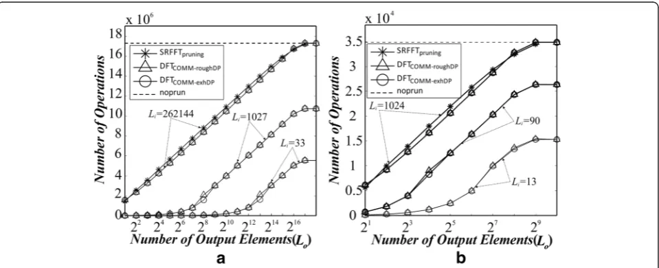
SRFFTprun-ing algorithm was developed for an implicit restriction that only a few consecutive output components (a num-ber L equal to a power of two) are required. Fig. 6 re-ports the number of arithmetic operations required to perform SRFFTpruning in comparison with our unified DFTCOMM method for multiple output pruning exam-ples using the decomposition factors (Dip,Dop) evaluated via the roughDP method and those specified by the exhDP method, respectively.
In both cases, it is considered that the DFTs of length P required by the intermediate stage of the pruned decomposed transform have been implemented by ap-plying the split-radix FFT, e.g., [26]. Therefore, the total number of arithmetic operations required by our pro-posed DFTCOMMmethod in comparison with the com-peting pruning-based algorithms can be found in Table 4. The savings in the number of arithmetic opera-tions attained with the new developed DFTCOMM tech-nique are reported in Tables 5 and 6.
From Fig. 6, one can deduce that our proposed DFTCOMM method requires fewer arithmetic operations than the competing SRFFTpruning method in almost all the test cases (with the only one exception for the case Lo=N/2 and Lo=N/4). Next, Tables 5 and 6 report the savings in the number of arithmetic operations attained with our DFTCOMMin comparison with the competing
Fig. 6Number of arithmetic operations required to perform the DFTCOMM, SRFFT(noprun), and the SRFFTpruningalgorithms; parametersDipand Dopare selected using roughDP and exhDP methods for a constant value ofLi, and different tested values ofLo= {21, 22,…,N}:aforN= 262,144
SRFFT and the SRFFTpruningtechniques. In the scenarios with Lo=N and Li= {21, 22,…, N}, the DFTCOMM algo-rithm manifests 2.96 and 2.73 % savings in the number of arithmetic operations in comparison with the SRFFTpruningforN= {262,144, 1024}, respectively.
In other cases, from Table 5, it follows that in the scenarios with Li= 1027, Li= 33, and Lo= {21, 22,…, N}, the SRFFTpruning method fails to deliver a result at all. Thus, from Table 5, it follows that in the cases when Li=N =262,144, Li= 1027, Li= 33, and Lo= {21, 22,…, N}, the DFTCOMM algorithm produces savings of 42.76, 75.02, and 91.35 %, respectively, in the number of arithmetic operations required to compute the composite length DFT in comparison with the com-peting SRFFT algorithm. Furthermore, from Table 6, it follows that in the scenarios with Li= 90, Li= 13, and Lo= {21, 22,…, N}, the SRFFTpruning method fails to deliver a result at all. Thus, from Table 6, it follows that in the cases whenLi=N= 1024,Li= 90,Li= 13, and Lo= {21, 22,…,N}, the DFTCOMMalgorithm produces sav-ings of 36.48, 59.30, and 81.65 %, respectively, in the
number of arithmetic operations required to compute the composite length DFT in comparison with the com-peting SRFFT algorithm.
Yuan et al., in [14], proposed another competing, the so-called SRFFTpruning−time−shift method via modifying the SRFFTpruning employing a time shifting approach that yields the input pruning algorithm based on the SRFFT methodology for L consecutive non-zero input elements. It is noteworthy to stress that the SRFFTpruning−
time−shiftapproach implicitly assumes that lengthsL andN may take values equal to the power of two only.
Figure 7 reports the number of required arithmetic op-erations to execute our proposed unified DFTCOMM method and those required by the competing pruned DFTs of [14]. These results verify that our approach re-quires fewer arithmetic operations than those required to perform the SRFFTpruning−time−shiftalgorithm in all the reported tests. Again, it is implicitly assumed that the DFTs of length Pinvolved in the DFTDIT−DIF−Prused by our DFTCOMMhave been computed using the split-radix FFT [26], as reported in Table 4.
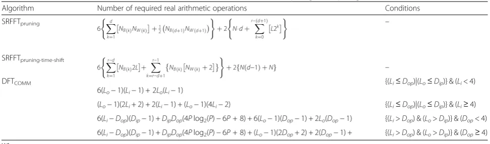
Table 4Total number of arithmetic operations required to compute the SRFFTpruning, SRFFTpruning-time-shift, and DFTCOMMalgorithms
Algorithm Number of required real arithmetic operations Conditions
SRFFTpruning
•N→Length of the full transform •r= log2(N)→Number of stages •L =2d
→Number of consecutive outputs that should be computed for SRFFTpruningalgorithm or number of consecutive non-zero inputs for SRFFTpruning-time-shiftalgorithm •Li→Number of consecutive input elements different from zero
•Lo→Number of consecutive output that should be computed •DipandDop→Integer decomposition factors
•N/DipDop≡P
Table 5Savings in the number of arithmetic operations attained with the DFTCOMMalgorithm in comparison with the competing
SRFFT (noprun) and SRFFTpruningmethods forN= 262,144
DFTCOMMin comparison with: Lo Li Savings
SRFFT(noprun) {21,22,…,N} N= 218 DFTCOMM, 42.76 % with output pruning
SRFFTpruning DFTCOMM, 2.96 % with output pruning
SRFFT(noprun) 1027 DFTCOMM, 75.02 % with input-output pruning at the same time
SRFFTpruning SRFFTpruningfails to deliver a result
SRFFT(noprun) 33 DFTCOMM, 91.35 % with input-output pruning at the same time
Next, Tables 7 and 8 report the savings in the number of arithmetic operations attained with our DFTCOMM in comparison with the competing SRFFT and the SRFFTpruning−time−shifttechniques. In the scenarios with Lo=N and Li= {21, 22,…, N}, the DFTCOMM algo-rithm manifests 5.11 and 8.71 % savings in the num-ber of arithmetic operations in comparison with the SRFFTpruning−time−shiftforN= {262,144, 1024}, respectively.
In other test cases, from Tables 7 and 8, it follows that for Lo= {1027, 90}, Lo= {33, 13}, and Li= {21, 22,…, N}, the SRFFTpruning−time−shiftalgorithm fails to deliver a re-sult at all. Furthermore, from Table 7, it follows that in the scenarios with Lo= {N, 1027, 33} and Li= {21, 22,…, N}, our DFTCOMM attains 43.26, 76.24, and 92.11 % savings for N= 262,144, respectively, in the number of arithmetic operations required to compute the compos-ite length DFT. In addition, from Table 8, it follows that in the scenarios withLo= {N, 90, 13} and Li= {21, 22,…, N}, our DFTCOMMattains 38.22, 59.22, and 82.45 % sav-ings for N= 1024, respectively, in the number of arith-metic operations required to compute the composite length DFT.
Note that our DFTCOMM always requires fewer arith-metic operations than the competing SRFFTpruning and SRFFTpruning−time−shift algorithms due to the different butterfly schemes employed to implement the split-radix FFT algorithms [26] and the unified commutation-pruning technique employed (see Section 3). The SRFFTpruning and SRFFTpruning−time−shift algorithms perform the two-butterfly scheme [26], while our DFTDIT−DIF−Pr algorithm employs the three-butterfly scheme to achieve a reduction in the number of arithmetic operations required to implement the DFTP blocks. Furthermore, graphs of Fig. 6 report that the SRFFTpruning algorithm fail to deliver a re-sult at all in the scenarios with L equal to N due to their algorithmic construction as reported by the au-thors of [3]. For this reason, this algorithm cannot present a valid value for the last test of Lo (it is sim-ply unable to stop to prune at all). In addition, Fig. 6 reports minimal differences between the numbers of arithmetic operations attained by the DFTCOMM evaluated using the roughDP- or exhDP-based selec-tion for specifying Dip and Dop. In summary, the
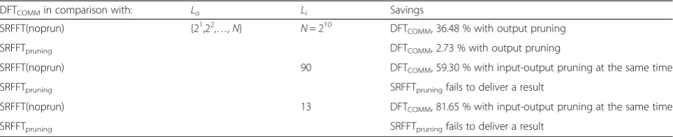
Table 6Savings in the number of arithmetic operations attained with the DFTCOMMalgorithm in comparison with the competing
SRFFT (noprun) and SRFFTpruningmethods forN= 1024
DFTCOMMin comparison with: Lo Li Savings
SRFFT(noprun) {21,22,…,N} N= 210 DFT
COMM, 36.48 % with output pruning
SRFFTpruning DFTCOMM, 2.73 % with output pruning
SRFFT(noprun) 90 DFTCOMM, 59.30 % with input-output pruning at the same time
SRFFTpruning SRFFTpruningfails to deliver a result
SRFFT(noprun) 13 DFTCOMM, 81.65 % with input-output pruning at the same time
SRFFTpruning SRFFTpruningfails to deliver a result
Fig. 7Number of arithmetic operations required to perform the DFTCOMM, SRFFT(noprun), and the SRFFTpruningalgorithms; parametersDipand Dopare selected using roughDP and exhDP methods for a constant value ofLo, and different tested values ofLi= {21, 22,…,N}:aforN= 262,144
number of arithmetic operations required to compute the SRFFTpruning, SRFFTpruning-time-shift, and DFTCOMM algo-rithms can be found in Table 4.
4.2 Comparison with the SFFT-related algorithms
In a context of pruned DFTs, real-world sensing scenar-ios are characterized by the uncertainties attributed to zero-padded input data acquisition modes with variable composite length windowing of the input and/or output Fourier transform sequences, in general cases, with non-sparse Fourier spectrum [10–12]. In contrast, the celebrated SFFT method developed and featured in [20] presumes “sparsity” of the Fourier spectrum that re-quires that majority of the Fourier coefficients are zeros or negligible; e.g., the authors of [20] exemplified such sparsity level at approximately 89 %, i.e., up to 89 % of the Fourier transform coefficients are to be zeroes or negli-gible for operability of their SFFT. Otherwise, the DFT should be specified and treated as anon-sparsetransform.
Currently, a family of novel efficient algorithms for computing the FFTs applicable for sparse sensing sce-narios when only a few Fourier transform coefficients (ks largest coefficients of the N-length Fourier trans-form) of the input signalx are different from zero have been developed [20, 21], which compose a family of the so-called SFFT methods. To compute a reliable SFFT for typical high N> 210, the sparsity level constraint re-quires that majority of the Fourier coefficients are zeros [20] (or negligible to be discarded). Such model as-sumptions are valid, for example, in video compressing applications [20]. Therefore, if majority of the Fourier transform coefficients are supposed to be zeros or can
be discarded, then efficient computing techniques from the SFFT family can be employed. The celebrated algo-rithms from such a family are the SFFTv1 and the SFFTv2 developed and featured in [20] where the spars-ity level was exemplified at 89 % of zero (negligible) Fourier coefficients. In [21], the SFFTv3 and SFFTv4 al-gorithms were proposed, where some computational improvements were introduced. SFFTv3 was imple-mented in [28] while the program code for implemen-tation of the SFFTv4 algorithm is not available at this time. Another competing technique for computing of the FFT of sparse (in the frequency domain) signals was addressed in [22] as the so-called FADFT-2 algorithm from the AAFFT library [22]. However, in [20, 21], it was corroborated that the SFFT-related algorithms manifest better operational performances than FADFT-2 of [22].
To perform valid test comparisons between the SFFTv1, SFFTv2, SFFTv3, and the DFTCOMM algo-rithms, those should be tested under the same condi-tions and constrains. Here, we use the following feasible constraints: the values of N vary as follows: N= {26, 27,…, 220} and ks=Lo, where Lo represents the number of consecutive output coefficients to be calculated. In different test scenarios, the SFFTv1, SFFTv2, and SFFTv3 algorithms deliver successful results: the first of them for N= {213, 214,…, 220} and ks=Lo= 50, the sec-ond of them for N= {213, 214,…, 220} and ks=Lo= 50, and finally, the third of them for N= {210, 211,…, 220} and ks=Lo= 50, respectively. Furthermore, it was ex-perimentally corroborated that the DFTCOMMalgorithm was able to deliver efficient results in all such tested sparse scenarios, as reported in Table 9.
Table 7Savings in the number of arithmetic operations attained with the DFTCOMMalgorithm in comparison with the competing
SRFFT (noprun) and SRFFTpruning-time-shiftmethods forN= 262,144
DFTCOMMin comparison with: Li Lo Saving
SRFFT(noprun) {21,22,…,N} N= 218 DFT
COMM, 43.26 % with input pruning
SRFFTpruning-time-shift DFTCOMM, 5.11 % with input pruning
SRFFT(noprun) 1027 DFTCOMM, 76.24 % with input-output pruning at the same time
SRFFTpruning-time-shift SRFFTpruning-time-shiftfails to deliver a result
SRFFT(noprun) 33 DFTCOMM, 92.11 % with input-output pruning at the same time
SRFFTpruning-time-shift SRFFTpruning-time-shiftfails to deliver a result
Table 8Savings in the number of arithmetic operations attained with the DFTCOMMalgorithm in comparison with the competing
SRFFT (noprun) and SRFFTpruning-time-shiftmethods forN= 1024
DFTCOMMin comparison with: Li Lo Saving
SRFFT(noprun) {21,22,…,N} N= 210 DFTCOMM, 38.22 % with input pruning
SRFFTpruning-time-shift DFTCOMM, 8.71 % with input pruning
SRFFT(noprun) 90 DFTCOMM, 59.22 % with input-output pruning at the same time
SRFFTpruning-time-shift SRFFTpruning-time-shiftfails to deliver a result
SRFFT(noprun) 13 DFTCOMM, 82.45 % with input-output pruning at the same time
In addition, DFT computations for other sparse test scenarios with different values ofN and ks were run, in particular, forN=Li= {213, 214,…, 217} andks=Lo= {1, 2,
…,ksmax} with ksmax= 11 % ofN. The test scenarios for the SFFT algorithms delivered successful results only for a few tested values of ks. For example, the SFFTv1 algorithm is executed successfully for N= {213, 215} and ks= {1, 2,…, 50}, for N= 214 and ks = {1, 2,
…, 50}∪{56, 57,…, 63}, for N= 216 and ks = {1, 2,
…, 50}∪{64, 65,…, 97}, and for N= 217 and ks= {1, 2,…, 74}.
The SFFTv2 algorithm is executed successfully for N= {213, 214,…, 217} and ks= {1, 2,…, 50}, while, the SFFTv3 algorithm performed successfully for N= 213 and ks= {4, 5,…, 673}, for N= 214 and ks= {4, 5,…, 1346}, for N= 215 and ks= {4, 5,…, 2692}, for N= 216 and ks= {4, 5,…, 5385}, and for N= 217 and ks= {4, 5,…, 10,771}. Furthermore, the DFTCOMM algorithm is executed successfully for all test cases (for N= {213, 214,…, 217} in combination with allks= {1, 5,…,ksmax}, as follows from the data reported in Table 10.
Table 11 reports the absolute average errors attained with the SFFTv1, SFFTv2, SFFTv3, and DFTCOMM algo-rithms, for N= {213, 214,…, 218} and ks=Lo= 50. In all test cases, the FFTW algorithm from [29] was used as a reference for computing the absolute error measures.
From the data reported in Table 11, it follows that for N= 8192 andks=Lo= 50, the SFFTv1 and SFFTv2 algo-rithms manifest very close absolute error values; in
particular, the attained average absolute error values were 5.6162 × 10⁻⁵ and 5.0689 × 10⁻⁵, respectively. However, the SFFTv3 attains a lower absolute average error values than other SFFT versions. It is noteworthy to mention that the lowest absolute average error was attained with the DFTCOMMalgorithm at a value of 2.7642 × 10⁻¹⁰.
In addition, Fig. 8 reports the absolute values of errors of the compared tested SFFTv3 and the DFTCOMM algo-rithms for N= 8192 and ks=Lo= 50 under the same sparse computing scenarios.
On the other hand, the SFFT-related algorithms demon-strate reliable operation for specific input parameter com-binations, i.e., they are dependent on the combination of the dimensionNof the input signalx, and the sparsity fac-torks. In contrast, the DFTCOMMalgorithm manifests the operational robustness in the sense that it does not subject to any of such dimensional limitation and demonstrated perfect operational performances in all tested harsh (non-sparse) computational scenarios. Furthermore, all SFFT-related algorithms are probabilistic-type techniques [20, 21], in which the desiredkslargest coefficients of the
Table 9Comparisons of the SFFTv1, SFFTv2, SFFTv3, and DFTCOMMalgorithms for different sizes (N) of the signalx, with N=Li= {2
(*) The program execution is aborted (✓) The program execution is successful
Table 10Comparisons of the SFFTv1, SFFTv2, SFFTv3, and DFTCOMMalgorithms for different sizes (N) of the signalx, with N=Li= {2
13
, 214,…, 217} andks=Lo= {1, 2,…,ksmax} in the tested
sparse scenarios withksmax~ 11 % ofN
Fourier spectrum of the input sequence are reconstructed (approximated) with a high probability (not mandatory with probability one). In contrast, the DFTCOMM algo-rithm is a deterministic technique, and it produces more reliable and accurate results than the family of the SFFT-related algorithms (as demonstrated in Fig. 8 and Tables 10 and 11).
It is also worthwhile to note that presently (in the sparsity-guaranteed computational scenarios only), the SFFT-related algorithms outperform the DFTCOMM in the computational speed due to their specially devised execution parallelism [20, 21, 28]. From the family of the SFFT-related algorithms, the SFFTv3 [28] manifests the most speed-up computational performances for any input sequence dimensionNand any feasible valueksin the sparsity-guaranteed scenarios only; in particular, when approximately only 8.2 % (or lower number) of the Fourier coefficients of the input signal are signifi-cant, thus not discarded (as shown in Table 10). In contrast, in all comparable (sparse or non-sparse) computational scenarios, the DFTCOMM algorithm manifested superior accuracy performances (lower absolute error values) than those attained with the SFFT-related algorithms.
In closing, it is noteworthy to mention that in a major-ity of practical computational scenarios, the savings in the number of arithmetic operations achievable with the optimized unified DFTCOMM technique are significant. As a concluding example, refer to the test scenario with N= 8192 and Li=Lo =307 in which case the savings in the total number of required arithmetic operations at-tainable with the DFTCOMM algorithm in comparison with the most prominent competing split-radix FFT algorithm [3, 14, 23, 24] constitute 45 %.
5 Conclusions
We have developed a new technique that carries out an efficient computation of the DFTs of composite lengths of the input and/or output data sequences smaller than the dimension N of the full DFT/FFT. The addressed methodology unifies the commuting, filtering, and pruning paradigms yielding the new DFTCOMM method that out-performs the existing competing pruning-decomposition-based techniques in the sense of attainable savings in the number of required arithmetic operations.
Furthermore, our DFTCOMMmethod admits computing the DFTPblocks at the intermediate stage of the pruned decomposed transform using any existing FFT algorithm.
Fig. 8Measures of absolute error values attained with the SFFTv3 and DFTCOMMalgorithms in sparse scenarios forN= 8192 andks=Lo= 50:aSFFTv3
and DFTCOMM;bDFTCOMM
Table 11Average absolute errors attained in sparse scenarios with the SFFTv1, SFFTv2, SFFTv3, and DFTCOMMalgorithms forN= {2 13
, 214,…, 218} andks=Lo= 50
Li=N ks=Lo SFFTv1 SFFTv2 SFFTv3 DFTCOMM
AbsError AbsError AbsError AbsError
213 50 5.6162 × 10⁻⁵ 5.0689 × 10⁻⁵ 2.4973 × 10⁻⁵ 2.7642 × 10⁻¹⁰
214 50 7.0000 × 10⁻⁴ 6.3012 × 10⁻⁴ 4.9943 × 10⁻⁵ 1.8228 × 10⁻⁹
215 50 2.8526 × 10⁻⁴ 2.5407 × 10⁻⁴ 9.9883 × 10⁻⁵ 1.6704 × 10⁻⁸
216 50 3.7305 × 10⁻⁴ 3.6885 × 10⁻⁴ 1.9976 × 10⁻⁴ 1.5567 × 10⁻⁷
217 50 4.9801 × 10⁻⁷ 4.8631 × 10⁻⁷ 1.5437 × 10⁻⁷ 2.6652 × 10⁻¹⁰
Based on the performed treatment of the combinational hypotheses testing-type problem regarding all feasible allocation-pruning modalities, the decision in favor of the preferable hypothesis was made that yields the proposed DFTCOMM method. Being the globally optimal decision making result of testing the complete list of all feasible hy-potheses, the DFTCOMM method guarantees to require a fewer or at most the same number of arithmetic opera-tions for its execution than any other of the competing pruning-decomposition-based methods reported in the literature.
In addition, we have corroborated that, in the scenarios with non-guaranteed sparsity of the data Fourier spectra, the DFTCOMMmethod manifests better reliability and ac-curacy than the family of the celebrated competing SFFT-related algorithms; while in scenarios with severe Fourier spectrum non-sparsity (i.e., when the majority of the data Fourier spectrum coefficients take non-zero values, thus cannot be discarded), the DFTCOMM technique always outperforms the celebrated SFFT-related algorithms be-cause all those simply fail to execute the program code in such uncertain computational scenarios.
6 Appendix
6.1 Main function
Fig 9 presents the pseudo-code of the main function that commute among the different alternatives to compute the DFTN (DFTCOMM). When the pruned decomposed transform is not required (Li≤DoporLo≤Dip), the direct method or the 2BF filtering method could be employed. In both cases, the Fourier coefficient X(0) is computed as a simple addition of the elements in the input se-quencex(n).
The directFourier function is used in the scenarios withLi< 4 to compute the remaining Fourier coefficients (k= 1:1:Lo−1). The 2BF filtering method is implemented when Li≥4. The directFourier function carries out the addition of complex multiplications of elements in x(n) by the complex exponentialWNnkdefined in (1). The fil-terFourier function computes each Fourier coefficient by implementing a recursive algorithm similar to the second-order Goertzel algorithm of [25]. In the filter-Fourier function, the feedback signal is multiplied by the real part of the complex exponentialsWNkand, next, by the conjugate of WNm. In our modification, the array of complex exponentials WNm is pre-computed for m= 0:1:N−1 and stored by duplicating in the vector W of length 2N (W= [WNm, WNm]), in such a way that WNnk and WNk could be read from it using nk and k as in-dexes, respectively. Accessing an element out of the vec-torWis impossible for these cases, as verified next. Liis inferior than 4 (or equivalently Li≤3) when the direct method is used, thus n≤Li−1≤2 andk≤Lo−1≤N−1,
and consequently nk≤2(N−1) < 2N. This assures that each element of WNnkcan be extracted from Wjust via accessing the element indexed by nk. Similarly, for k≤ Lo−1≤N−1, each element ofWNk is directly extracted fromWaccessing the element indexed byk. In order to
avoid multiplications in the generation of the index,nk, the latter is computed by addingktonkin each iteration of the loopn(inside the function directFourier).
In the scenarios with Li>Dop and Lo>Dip, the DFTDIT−DIF−Pr is performed to compute the DFTN. As it was explained previously, the DFTDIT−DIF−Pr is per-formed in three commuting stages: the input stage, the intermediate stage, and the output stage. These stages are executed in a sequential order by calling the InputStage Fig. 10Pseudo-code of the InputStage function
function, next the IntermediateStage function, and, finally, the OutputStage function.
6.2 InputStage function
The InputStage function generates the inputs to the intermediateDipDopDFTs of lengthP (DFTPs), resulting in an array of three dimensions y(n1, n2, k1). The pseudo-code for implementing the InputStage function is listed in Fig. 10. The indexes,n1, n2, andk1are varied using three nested loops (“for” instructions), in such an order that the number of accesses to each element in x(n) is reduced. This is achieved by specifyingk1for the inner loop, n1for the intermediate loop, and n2for the outer loop. With this order, once an element in x(n1+ Dopn2) is loaded, all the inputs of the DFTPs that depend on it are generated. To minimize the required computa-tions, the nested loops have been broken down to avoid multiplications by one and the application of if-clauses.
In order to avoid overhead in the generation of the in-dexes, those are generated by additions only. After the InputStage function has been executed, the intermediate stage should be called.
6.3 Intermediate stage function
The intermediate stage consists in computing Dip -DopDFTs of lengthP=N/DipDop. This stage could be im-plemented with any algorithm for computing a DFT. For instance, the split-radix could be used if Pis a power of two [26] or the radix-3 could be used ifP is a power of three [27]. For a general case, we recommend using the FFTW (the fastest Fourier transform in the west) re-ported in [29] to compute theDipDopDFTPs since this is the most efficient algorithm for an arbitrary length DFT. The selected algorithm should be applied over each vec-tor obtained fromy(n1, 0 : 1 :P−1,k1) for each value of n1andk1, resulting in a vector with output indexk2that is stored in the array z(n1, k2, k1). This array is then processed by the OuputStage function.
6.4 OutputStage function
The OutputStage is performed to compute the final Fourier coefficients from the outputs of the Dip -DopDFTPs stored inz(n1, k2, k1). This function is listed in Fig. 11. In fact, the OutputStage function performs the computation of another stage of DFTs, although with a few outputs. As previously mentioned, there are two alternatives to compute each Fourier coefficient from z(n1, k2, k1), using a direct computation or using the 2BF filtering method. Thus, the OutputStage func-tion could employ the direct-Fourier or the filterFourier functions listed in the pseudo-code of Fig. 9 to compute the final Fourier coefficients.
Each Fourier coefficient depends on Dop inputs (ob-tained fromz(n1,k2,k1) by varyingn1), so forDop< 4, the
direct method is desirable; otherwise, the 2BF filtering method is to be executed.
These nested loops should be implemented in the in-dicated order to specify the indexes of the final Fourier coefficients. Those indexes are obtained by increasing index k by a unit in each iteration of the loop indexed by k1. The directFourier function utilizes the complex exponential WNnk, while the filterFourier function in-volves the complex exponential WNk. All elements WNk and WNnk are extracted from W using k and nk as in-dexes, respectively. In order to reduce multiple copies of data and thus to achieve an enhanced efficiency of the algorithm, it is strongly desirable to implement inline functions and passing the arrays elements by reference instead of by value.
Competing interests
The authors declare that they have no competing interests.
Acknowledgements
The authors would like to thank the anonymous reviewers for their constructive criticism and comments that helped to improve the presentation of the paper.
Received: 30 March 2015 Accepted: 11 November 2015
References
1. J Markel, FFT pruning. Audio and Electroacoustics, IEEE Transactions on 19(4), 305, 311 (1971). doi:10.1109/TAU.1971.1162205
2. V Raghavan, KMM Prabhu, PCW Sommen, Complexity of pruning strategies for the frequency domain LMS algorithm. Signal Processing86(10), 2836–2843 (2006). ISSN 0165–1684, http://dx.doi.org/10.1016/j.sigpro.2005.11.015 3. Y Xu; M-S Lim, Split-radix FFT pruning for the reduction of computational
complexity in OFDM based cognitive radio system,in Proceedings of 2010 IEEE International Symposium on Circuits and Systems (ISCAS), 69-72, May 30-June 2 2010. doi: 10.1109/ISCAS.2010.5537048.
4. FM Henderson, AV Lewis (eds.),Principles and applications of imaging radar, manual of remote sensing, vol. 3, 3dth edn. (Willey, NY, 1998)
5. HH Barrett, KJ Myers,Foundations of image science(Willey, NY, 2004) 6. YV Shkvarko, Unifying experiment design and convex regularization
techniques for enhanced imaging with uncertain remote sensing data–– part I: theory, part II: adaptive implementation and performance issues. IEEE Trans. Geoscience and Remote Sensing48(1), 82–111 (2010)
7. A Moni, CJ Bean, I Lokmer, S Rickard, Source separation on seismic data. IEEE Signal Processing Magazine29(3), 16–28 (2012)
8. RM Willet, MF Duarte, MA Davenport, RG Baraniuk, Sparsity and structure in hyperspectral imaging. IEEE Signal Processing Magazine31(1), 116–126 (2014) 9. Q Zhu, CR Berger, EL Turner, L Pileggi, F Franchetti, Polar format synthetic
aperture radar in energy efficient application-specific logic-in-memory,IEEE International Conference on Acoustics, Speech and Signal Processing (ICASSP), 2012, pp. 1557- 1560, 25–30 March 2012. doi: 10.1109/ICASSP.2012.6288189. 10. YV Shkvarko, J Tuxpan, SR Santos, I Yaniez,High-resolution imaging with
uncertain radar measurement data: a doubly regularized compressive sensing experiment design approach,in IEEE Intern. Symposium on Geoscience and Remote Sensing (IGRSS’2012), Munich, Germany, 6976–6970. (2012). ISBN: 978-1-46731159-51/12
11. YV Shkvarko, J Tuxpan, SR Santos,l2-l1Structured descriptive experiment design regularization based enhancement of fractional SAR imagery. Signal Processing93, 3553–3566 (2013). http://dx.doi.org/10.1016/j.sigpro.2013.03.024 12. S Foucart, H Rauhut,A mathematical introduction to compressive sensing
(Springer, NY-Heidelberg, 2013)
14. L Yuan, X Tian, Y Chen, Pruning split-radix FFT with time shift, International Conference on Electronics, Communications and Control (ICECC), 2011, 1581-1586, 9–11 Sept. 2011. doi: 10.1109/ICECC.2011.6066654.
15. S Bouguezel, MO Ahmad, MNS Swamy, Efficient pruning algorithms for the DFT computation for a subset of output samples,in Proceedings of the 2003 International Symposium on Circuits and Systems, 2003. ISCAS '03, vol.4, pp. IV-97, IV-100 vol.4, 25–28 May 2003. doi: 10.1109/ISCAS.2003.1205782. 16. C-P Fan, G-A Su, Pruning fast Fourier transform algorithm design using
group-based method, Signal Processing87(11), 2781–2798 (2007), ISSN0165-1684, http://dx.doi.org/10.1016/j.sigpro.2007.05.012
17. TV Sreenivas, P Rao, FFT algorithm for both input and output pruning, in IEEE Transactions on Acoustics, Speech and Signal Processing,27(3), 291–292 (1979). doi:10.1109/TASSP.1979.1163246
18. C Roche, A split-radix partial input/output fast Fourier transform algorithm, in IEEE Transactions on Signal Processing,40(5), 1273, 1276 (1992). doi:10. 1109/78.134493
19. L Wang, X Zhou, GE Sobelman, R Liu, Generic mixed-radix FFT pruning, in IEEE Signal Processing Letters,19(3), 167, 170 (2012). doi:10.1109/LSP.2012. 2184283
20. H Hassanieh, P Indyk, D Katabi, E Price, 2012. Simple and practical algorithm for sparse Fourier transform, inProceedings of the twenty-third annual ACM-SIAM symposium on Discrete Algorithms(SODA '12) Kyoto, Japan, 17-19 Jan, 1183–1194, (2012)
21. H Hassanieh, P Indyk, D Katabi, E Price, Nearly optimal sparse Fourier transform, inProceedings of the forty-fourth annual ACM symposium on Theory of computing (STOC '12), ACM, New York, (2012), 563–578. doi:10.1145/2213977.2214029. http://doi.acm.org/10.1145/2213977.2214029 22. M Iwen, A Gilbert, M Strauss et al., Empirical evaluation of a sub-linear
time sparse DFT algorithm, Communications in Mathematical Sciences 5(4), 981–998 (2007)
23. HV Sorensen, CS Burrus, Efficient computation of the DFT with only a subset of input or output points, in IEEE Transactions on Signal Processing, 41(3), 1184–1200 (1993). doi:10.1109/78.205723
24. M Medina-Melendrez, M Arias-Estrada, A Castro, Input and/or output pruning of composite length FFTs using a DIF-DIT transform decomposition, in IEEE Transactions on Signal Processing,57(10), 4124, 4128 (2009). doi:10.1109/TSP.2009.2024855
25. AV Oppenheim, RW Schafer, Discrete-time signal processing, (Prentice Hall, 2nd Edition, U.S., 1999)
26. HV Sorensen, M Heideman, CS Burrus, On computing the split-radix FFT, in IEEE Transactions on Acoustics, Speech and Signal Processing,34(1), 152–156 (1986). doi:10.1109/TASSP.1986.1164804
27. Y Suzuki, S Toshio, K Kido, A new FFT algorithm of radix 3,6, and 12, in IEEE Transactions on Acoustics, Speech and Signal Processing,34(2), 380–383 (1986). doi:10.1109/TASSP.1986.1164826
28. J. Schumacher, M. Püschel, High performance sparse fast Fourier transform, Master´s thesis, ETH Zurich, Department of Computer Science (2013). 29. M Frigo, SG Johnson, The design and implementation of FFTW3, Proceedings
of the IEEE93(2), 216–231 (2005) doi:10.1109/JPROC.2004.840301
Submit your manuscript to a
journal and benefi t from:
7 Convenient online submission
7 Rigorous peer review
7 Immediate publication on acceptance
7 Open access: articles freely available online
7 High visibility within the fi eld
7 Retaining the copyright to your article