A weighted eigenvector autofocus method for sparse aperture ISAR imaging

R E S E A R C H

Open Access

A weighted eigenvector autofocus method for

sparse-aperture ISAR imaging

Jia Duan

, Lei Zhang and Meng-dao Xing

Abstract

With the development of multi-functional radar systems, inverse synthetic aperture radar (ISAR) imaging with sparse-aperture (SA) data has drawn considerable attention in the recent years. Motion compensation and imaging are among the most significant challenges that SA-ISAR imaging frequently faces. In this paper, we focus on the autofocus scheme, in which a modified eigenvector-based autofocus method is proposed. In the method, different weights are endued to different range cells according to their signal-to-noise ratios (SNRs). Using the weights, the contribution from the range cells with high SNR is enhanced, yielding accuracy improvement in phase error estimation. What is more is that to improve the estimation precision, an iterative scheme is introduced.

Experimental results show that the proposal is not only robust to severe noise but also applicable to ISAR imaging with different SA patterns. Detailed comparisons are given in order to show the superiorities of the proposal in phase adjustment for ISAR data.

Keywords:Inverse synthetic aperture radar (ISAR), Autofocus, Sparse aperture (SA), Weighted eigenvector phase adjustment

1. Introduction

Inverse synthetic aperture radar (ISAR) has the capabil-ity of producing high-resolution images of noncoopera-tive targets in all weather conditions. However, a considerably high-resolution ISAR image is only obtain-able when enough pulses are continuously measured. Unfortunately, for a modern radar system, this is diffi-cult: (1) Long coherent processing interval is usually un-achievable due to the uncooperative property of ISAR targets. (2) Multi-sourced interferences may contaminate some portions of the received pulse seriously. These por-tions must be removed in case of false points and blurred images, resulting in discontinuous measure-ments. (3) With the development of modern multi-mode and multi-functional radar systems, spending long con-tinuous observation time on a single-target measure-ment is no longer acceptable. Moreover, when multiple targets present simultaneously, the radar systems have to switch among different lines of slight to capture multiple targets. Therefore, for modern radar systems, received

pulses for a single target are usually very limited and even discontinuous.

Due to these constraints on data collection, sparse-aperture (SA) samples are introduced in modern ISAR systems. Therefore, in order to increase the flexibility and robustness of modern radar systems, the study on sparse-aperture ISAR (SA-ISAR) imaging is urgent. In general, there are two major problems confronting SA-ISAR imaging.

The first one lies in the way of obtaining full-aperture -resolution ISAR images with SA measurements. To handle this, several methods are proposed, which can be divided into two major categories. The first category is the compressive sensing-based high-resolution SA-ISAR imaging methods [1-6]. These methods are able to achieve an exact or close recovery of signal by solving a

minimum l1 optimization problem. The other kind of

useful technique for full-aperture signal reconstruction is spectral analysis algorithm [7,8]. One of the most well-known techniques is the gapped-data amplitude and phase estimation method, which estimates the inte-grated spectrum by designing narrowband filters to interpolate missing data [8].

* Correspondence:[email protected]

National Key Lab of Radar Signal Processing, Xidian University, Xi’an 710071, People's Republic of China

The second problem confronting SA-ISAR imaging is motion error compensation. Due to the discontinuous sampling process, motion error compensation becomes much more complex in SA-ISAR. Motion error compen-sation can be achieved by range alignment and phase ad-justment. Range alignment is used to remove the range migration of different pulses, while phase adjustment is used to correct their phase errors. It should be empha-sized that several existing range alignment methods are already capable to correct range migrations for SA-ISAR data [9-11]. With respect to phase adjustment, there are lots of phase compensation methods available for con-ventional ISAR. The famous phase gradient autofocus (PGA) method can approximately reach the Cramér-Rao boundary by five or six iterations [12]. The weighted least squares method is a robust algorithm without any requirements on the noise model [13]. However, neither one is suitable for the SA case. To our knowledge, the study on the phase compensation methods for SA-ISAR is quite few. Among the conventional autofocus methods, the eigenvector method is proven to be applicable for SA-ISAR phase error estimation [14,15]. In the eigenvector-based phase correction method, the maximum likelihood (ML) principle is used, resulting in a solution involving the eigenvector corresponding to the prominent eigen-value of the sample covariance matrix. Nevertheless, its performance is dependent on the noise level and SA pat-terns of available samples. To improve the eigenvector-based phase adjustment, a weighted eigenvector-eigenvector-based phase correction method is addressed in this article. In this method, weights are designed to encourage the contri-bution of range cells with high signal-to-noise ratio (SNR) and suppress that of range cells with low SNR, yielding a more precise and stable estimation. As an optimal candi-date for the SA-ISAR phase adjustment, the weighted eigenvector method performs well in adverse circum-stances, such as highly noisy and SA cases. After motion compensation by the proposed autofocus approach, an SA-ISAR imaging method is applied to coherently focus SA-ISAR data for full-aperture-resolution image [3]. The imaging results of simulated and measured data validate the effectiveness of the proposed method.

The remainder of this paper is organized as follows: In the‘Signal model for SA-ISAR’section, the signal model

for SA-ISAR is introduced. In the‘Weighted eigenvector method for phase error correction’section, both the the-ory principle and operation flow of the weighted eigen-vector algorithm are illustrated. Moreover, a simple description of the SA-ISAR imaging scheme [3] has been described. In the ‘Performance analysis’ section, auto-focusing and imaging experiments are carried out with acquired ISAR data sets. By comparing with other auto-focus algorithms, the superiority of the improved method is shown. Finally, some conclusions are drawn in the last section.

2. Signal model for SA-ISAR

Considering that a monostatic ISAR system observes multiple targets simultaneously, the radar has to switch among different targets during the observing time, resulting in SA for each target.

Let fxkð Þm gMm¼10 denote the kth complete aperture

range cell with lengthM0. It can be regarded as a long vector withPsub-apertures,

xk¼Δ _xk 1

ð Þ xkð Þ2 ⋯ xkðM0Þ

½ T_¼Δ _xT

k1 xTk2 ⋯ xTkP

T_;

ð1Þ

where xTk1;xTk2;⋯;xTkP are sub-vectors of xk, whose

lengths are L1, L2,⋯,LP, respectively, with L1+L2+⋯+ LP=M0. Assume that the even sub-apertures of xk are

missing due to the radar working mode, and an SA vec-torγkis formed as follows:

γk¼

Δ _xT

k1 xTk3 ⋯ xTkP

T_{: ð}

2Þ

Let μ_k¼Δ _xT

k2 xTk4 ⋯ xTkP−1

T

denote the missing aperture samples, andPis supposed to be odd for the con-venience of the following derivation. Let γk and μk have

lengths of M and M0−M, respectively, where M is the total number of available samples withM=L1+L3+⋯LP.

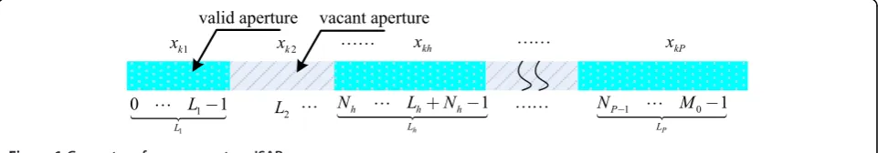
Figure 1 shows the geometry of the SA-ISAR, in which the full aperture containsM0pulses with an index from 0 toM0−1. The odd sub-apertures are available, and the hth sub-aperture consists of Lh pulses, whose index is

fromNhtoNh+Lh−1.

3. Weighted eigenvector method for phase error correction

In conventional ISAR processing, motion compensation usually begins in the range-compressed phase-history domain. Thus, range alignment is implemented to the range-compressed SA data firstly by some novel ap-proaches [9-11], which are proven to be effective even for SA data.

By referring to [14], a signal model for phase error es-timation is introduced, in which each dominant range cell contains a single dominant scattering center and other clutters are modeled as uniform-intensity Gaussian white noise. These dominant range cells are usually uti-lized to estimate phase errors because of their high SNR properties. From [11], a range cell whose normalized amplitude variance is less than 0.12 (0.2) can be referred to as a dominant range cell.

Hence, the sparsely sampled lth dominant range cell after range compression is given as

γl¼

Δ al ej

φ1þ2πfl1

ð Þ

ejðφ2þ2πfdl⋅t1Þ

⋯ejðφmþ2πfdl⋅tmÞ⋯ejðφMþ2πfdl⋅tMÞ

#

þnl; ð3Þ

"

where al represents the complex amplitude of the lth

dominant range cell; nl denotes the interference from

noise, which follows a Gaussian distribution with vari-ance δ2_l; Doppler frequency is denoted byfdl; and phase

error at azimuth positionmisφm.

Suppose that L dominant range cells are chosen for estimation. For the convenience of deduction, we as-sume that the Doppler shift of each dominant range cell has been removed temporarily. The Doppler shift re-moval scheme will be subsequently discussed in the ‘Elimination of Doppler shift’section. Then, the range-compressed dominant echoes can be expressed by

X¼½γ1 ⋅⋅⋅ γl ⋅⋅⋅ γL ML

¼vM1⋅α1LþNML; ð4Þ

where the phase error vector is symbolized by v with

vM1¼ejð Þφ1 _ejð Þφ2 ⋅⋅⋅ _ejðφMÞT. Note that the phase

error is constant across all dominant range cells. The

complex amplitude vector is denoted by α_1L

¼½a1 ⋯ aL, andNstands for the complex

Gauss-ian white noise matrix. Generally, the noise in each dominant range cell is an independently and identically distributed Gaussian random variable. Therefore, we let

δ2 1¼δ

2

2¼…¼δ 2

L¼δ

2_{. By this, the covariance matrix}

of noise can be computed as δ2I [13], symbolizing as cov(N).

3.1. Weighted eigenvector method

3.1.1. Independent phase error elimination

Based on the assumption in the last sub-section, thelth dominant range cell for SA-ISAR is expressed as

γl¼alejð Þφ1 _ejð Þφ2 ⋅⋅⋅ _ejðφMÞTþn_l

¼alvM1þnl: ð5Þ

Let C^ ¼1_LXXH¼_L1X

L

l¼1

γlγHl . It has been proven that

the ML estimation [9] ofvis to choosevmaximizing (6) withvHv=M,

Q¼vHCv^ ¼X

M

m¼1

λmj jzm2: ð6Þ

Define zas z¼½z1 ⋯ zMT¼PHv, of which Pis

the eigenmatrix ofC^ [5].

Clearly, (6) is maximized for zmax such that |zm|2=M

and |zk|2= 0 fork≠m, wheremis the index

correspond-ing to the largest eigenvalueλmofC^. That is,zTmax¼M⋅

ejθ _{0;⋯; 1}

mth;⋯;0

h i

, whereθis an arbitrary rotation angle.

Therefore, the ML estimation of v is vmax=M ejθpm, in

whichpmis the significant eigenvector ofC^. After

apply-ingpmto correct the phase error, phases are compensated

to a constant. Namely, phase adjustment is achieved. In [15], the eigenvector method is validated to be suitable to correcting phase errors for SA-ISAR data.

It should be emphasized that each dominant range cell is fairly treated in the eigenvector-based phase error esti-mation method. However, for SA-ISAR, there are several dominant range cells with relatively high SNRs. With high SNR property, these dominant range cells are cap-able of providing more precise information for phase error estimation than others. Based on this, an improved eigenvector autofocus method is established. The im-provement involves a weighted optimization function for estimating the phase error. From (6), in order to obtain a more precise estimation, one needs to enhance the contributions of signals and suppress those of noise in the calculation of C^ . This can be accomplished by adding significant weights to the dominant range cells with high SNRs, which will be discussed elaborately as follows.

In order to obtain an adjusted C^, we add weights to each dominant range cell. Let εl(l= 1, 2,⋯,L) represent

the weight for thelth cell, then

X0_{¼ ε}

1γ1 ⋅⋅⋅ εLγL

ML¼v⋅a

0_þN0_{; ð7Þ}

where the weighted complex amplitude is symbolized by α' with α0¼½ε1a1 ⋯ εLaL and weighted noise

matrix is denoted by N0¼½ε1n1 ⋯ εLnL. The

with ease, i.e., covð Þ ¼N0 1

rithm of conditional probability density function for the weightedX' givenvis provided as

lnpðX0j Þ ¼v −NlnπMj jC0−X

whereC' denotes the covariance matrix of the weighted data,

, the inverse matrix of C' is computed

as

By substituting (10) into (8), the weighted ML optimal problem has been converted into finding a vector v, which maintains the following equation most likely:

Q0¼X

ivation of the eigenvector method, the solution of (11) is related to the eigenvector corresponding to the promin-ent eigenvalue of C^0, after scaling its squared modulus to M. Namely, ^v¼Mejθ1p

m0, where pm' is the largest

eigenvector of C^0 and θ1 is an arbitrary rotation angle. Instituting ^v into (11),Q' obtains its peak valueλ'maxM,

change the total energy. Here, weight is chosen directly proportional to SNR, which is defined as the ratio of the dominant scatterer energy to the total noise energy in

the cell, namelyω_l¼κa2l

δ2 L

[16,17]. A notable point is that

the energy of noise includes both that of weak scatterers and clutters. In order to hold the total energy still,κcan

be normalized as∑γH_l γ_l=∑a

For the sake of comparison, the SNR after weighting can be calculated as follows:

XL

On the assumption that the noise in each range cell is independently and identically distributed, we have δ2₁

¼δ2

2¼…¼δ 2

L¼δ

2_{. After substituting it into (12), it}

can be obtained that

XL

Because of the lemma that LX

L

a2_l≥0. The detailed derivation of

the lemma is listed as follows:

XL

After substituting L⋅X

L

been improved by the weighting processing compared with that of C^. In this way, the maximum eigenvalue

with (6), a more precise phase adjustment is resulted in than before.

3.1.2. Elimination of Doppler shift

On the assumption that the Doppler shift of each dom-inant range cell is removed, the weighted eigenvector-based autofocus method is effective. However, the Doppler shift is relevant to the cross-range position of each dominant scattering center, which differs with both azimuth and range positions. So as to ensure the feasibility of our method, Doppler shift should be removed before the coherence matrix calculation.

In traditional ISAR phase error compensation methods, center shifting is utilized to reduce the influence of Doppler shifts, which works in two steps. Firstly, by Fourier transforming (FT), echoes are transformed into the range-Doppler (RD) image domain. Then, Doppler shift is removed by circularly removing each dominant scatterer to the center of the image. However, for SA-ISAR, especially when it comes to the unevenly under-sampling cases, the method needs some modification. Because of the discontinuous phase history, it is impos-sible for the SA-ISAR signal to be coherently accumulated by FT. To handle this, zero padding is utilized [13]. In this way, FT can be useful, namely circularly shifting can be implemented. In this article, instead of circularly shifting, we multiply a corresponding linear-phase function with the zero-padded signal in the time domain. The linear-phase function is constructed by estimating Doppler shifts from the positions of strongest response in the RD do-main. Note that although the sidelobes are highly raised,

the mainlobe is still higher so that the positions can be de-termined. Finally, vacant apertures are removed from the product.

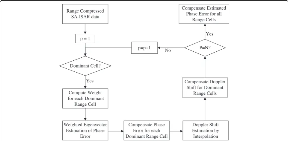
Nonetheless, due to the presence of phase error, the Doppler shift removal is not optimal as expected. There-fore, the phase error correction and Doppler shift esti-mation are done in a mutually iterative manner, in which one estimated variable is used to update the esti-mation of the other. Through this scheme, the Doppler shift and phase error are estimated and reduced grad-ually. Finally, with the increase of iteration number, pre-cise estimations are resulted in. For clarity, the flowchart of the weighted eigenvector autofocus method is shown in Figure 2.

Firstly, in order to determine which range cells are chosen as the samples for coherence matrix computa-tion, we compute the normalized amplitude variance of each range cell.

Secondly, the estimation of phase errors is done in two steps:

Step 1: Weight is calculated for each dominant range cell according to SNR. Then, the weighted covariance matrix is obtained, and the eigenvector corresponding to the largest eigenvalue is used to correct the phase errors roughly. Subsequently, Doppler shift is estimated and compensated. Step 2: Re-determine phase errors by the weighted

eigenvector autofocus method. After compensating the estimated phase error to the dominant range cells, Doppler shift is re-estimated and compensated.

Range Compressed SA-ISAR data

p = 1

Dominant Cell?

Compute Weight for each Dominant

Range Cell

Weighted Eigenvector Estimation of Phase

Error

Compensate Phase Error for each Dominant Range Cell

Doppler Shift Estimation by Interpolation Compensate Doppler

Shift for Dominant Range Cells

P=N? Compensate Estimated

Phase Error for all Range Cells

p=p+1 No

Yes

Yes

Continue the above sub-steps until the ceasing condi-tion is satisfied. The halt condicondi-tion may be the count of iteration number. Experimental results show that two or three iterations are enough to ensure the accuracy.

At last, we compensate the whole range cells with the estimated phase error.

3.2. SA-ISAR imaging

For traditional ISAR after autofocusing, RD imaging is a simple but effective method to obtain a well-focused image of targets. However, for SA-ISAR data with the sparsely sampled Doppler history, RD images of targets usually smear seriously with high gratinglobes and sidelobes. To reduce the discontinuous sampling effects on SA imagery, many novel approaches have been pro-posed. In [3], a sparsity-driven algorithm to generate high-resolution ISAR images is given, in which a SA-ISAR imaging problem is converted into a sparsity-constrained optimization problem based on the

max-imum a posteriori estimation. The optimization is given

as follows:

^

Að Þ ¼X arg max A∈CNM

− 1

2σ2kXFAk 2 2−γk kA 1

¼arg min

A∈CNM

XFA

k k2

2þμk kA 1

;

ð15Þ

where μ= 2σ2γ is the sparsity coefficient andγ is the La-place distribution parameter. They are directly related to the unknown statistics of noise and target signal.Xstands for the SA-ISAR echo matrix, as defined before.Fis a par-tial Fourier matrix, which can be easily constructed corre-sponding to the pattern of SA. A= [anm] is an N×M

matrix and denotes the two-dimensional (2D) ISAR image, whose pixel values are corresponding to scattering center amplitudes.

Based on the assumption that the additive noise is sub-ject to a zero-mean Gaussian distribution with unknown varianceσ2 and the signal components corresponding to the dominant scattering centers follow a Laplace distribu-tion with coefficient γ independently, it utilizes the constant-false-alarm-ratio detector to discriminate signal from noise in the sub-aperture images approximately. Using the pure noise and target components, bothσ2and

γcan be obtained via ML. In this SA-ISAR imaging algo-rithm, a modified quasi-Newton algorithm is applied in an iterative manner for image formation [4], and in order to improve the efficiency of the solver, fast Fourier transform and conjugate gradient algorithm are applied in its imple-mentation [3]. Real data experiments manifest the effect-iveness of the method. Therefore, we use this SA-ISAR imaging algorithm jointed with phase adjustment pro-posed to achieve a high-quality SA-ISAR image.

4. Performance analysis

In this section, real ground-based measurements are conducted to analyze the performance of the weighted eigenvector phase correction method. By considering different SA patterns, such as complete aperture pattern, unevenly SA pattern, and block SA pattern, the univer-sality of our method is investigated. The following exper-iments are vital to validate the effectiveness of our method.

4.1. Dataset and evaluation criterion

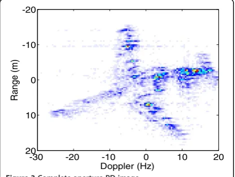
To make our experiments convincing, real measured ISAR data are used to perform different experiments. A dataset of Yak-42 airplane is used, which is recorded using a C-band (5.52GHz) ISAR experimental system. This system transmits a 100-MHz linear modulated chirp signal with 25.6-μs pulse width. The range reso-lution is 0.375m. The echo is de-chirped and I/Q sam-pled for range compression. After range compression, conventional range alignment and phase adjustment are applied to the complete aperture data. Then, RD im-aging method is implemented, producing a well-focused image, as illustrated in Figure 3. We use it as a standard image for evaluating the following experimental results.

After applying 2D inverse Fourier transforming to the well-focused image, random Gaussian phase error and white noise are added to generate defocused data sets with different SNRs. The added phases randomly vary within [−π, π]. Moreover, SA-ISAR data are created by extracting some pulses from the data sets in both ran-dom and block manners. Thus, the performance of phase correction methods under different conditions is analyzed.

In order to assess the performance quantitatively, cri-teria should be built. Since the entropy of an image is usually used as an index that quantitatively represents the information of the luminosity distribution of the

Doppler (Hz)

R

ange (m

)

-30 -20 -10 0 10 20

-20

-10

0

10

20

image, entropy criterion is used to analyze the perform-ance for the complete aperture case. However, owing to the use of parametric superresolution approaches, the image entropy criterion is not suitable to SA-ISAR im-ages [4]. Therefore, a criterion built in [13] is brought in to appraise the weighted eigenvector phase adjustment method for SA cases quantitatively:

pe¼

1 M

XM

m¼1

v mð Þ−^v mð Þ

j j2_{; ð}

16Þ

where pe is defined as the square error between esti-mated phase and added phase, andvand ^v are the ap-plied and estimated phase errors, respectively.

4.2. Experimental results and analysis

4.2.1. Performance under low SNR with complete aperture data

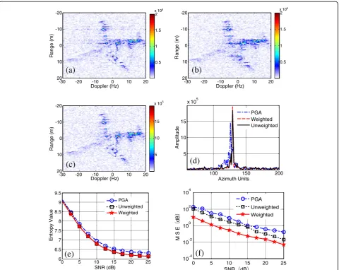
To testify the effectiveness of our method under low SNR, complex-valued Gaussian noise and phase error are added to generate degraded data set with 0-dB SNR. After range compression, three autofocus methods

(trad-itional eigenvector method, PGA algorithm, and

weighted eigenvector method) are performed to estimate the phase errors. Since we use complete aperture here, traditional RD imaging algorithm is adopted. The RD images with different phase adjustment methods (PGA, eigenvector, and weighted eigenvector methods) are shown in Figure 4a,b,c, respectively. Note that although the original eigenvector method can get highly focused results in certain range cells, blurring cases emerge in

0 5 10 15 20 25

6 6.5 7 7.5 8 8.5 9 9.5

SNR (dB)

Entropy Value

PGA Unweighted Weighted

Doppler (Hz)

R

ange (m

)

-30 -20 -10 0 10 20

-20

-10

0

10

20

0.5 1 1.5 2

x 106

Doppler (Hz)

R

ange (m

)

-30 -20 -10 0 10 20

-20

-10

0

10

20

0.5 1 1.5 2

x 106

Doppler (Hz)

R

ange (m

)

-30 -20 -10 0 10 20

-20

-10

0

10

20

5 10 15 x 105

(a)

(b)

(c)

100 150 200

5 10 15

x 105

Azimuth Units

A

m

p

lit

u

d

e

PGA Weighted Unweighted

0 5 10 15 20 25

10-4

10-2

100

102

104

SNR dB

M S E

dB

PGA

Unweighted Weighted

(d)

(e)

(f)

other range cells. This is improved by the weighted eigenvector method, which is better than the result of PGA as well.

For comparison, the 146th range cell with one domin-ant scatterer is chosen. The envelope of the 146th range cell is plotted in Figure 4d. It is obvious that the mainlobe of the proposed algorithm is the highest and the sidelobe is the lowest of the three methods. There-fore, the weighted method outperforms other methods under 0-dB SNR.

Furthermore, the performance of the three phase ad-justment methods under different SNRs is analyzed and compared by Monte Carlo simulation. At each generated SNR, a hundred independent experiments have been conducted. Entropy of the focused image is computed. Its definition is given in [18], which is

u¼∑

m∑n

A m;ð nÞ

j j2

S ln

S A m;ð nÞ

j j2

S¼∑

m∑njA m;ð nÞj

2_; ð17Þ

where u means the entropy value of an ISAR image, A (m,n) is the amplitude of pixel (m,n), andS is the total energy of the ISAR image.

The mean value of entropy with SNR is presented in Figure 4e. From the image, the proposed method is superior to others, especially under low SNRs. With the increased SNR, the entropy values decrease sharply and results of the three methods become similar. As to the comparison of the steadiness, Figure 4f shows the mean square error (MSE) of entropy varying with SNR, with which the results indicate that the proposed method is robust and stable under low SNR conditions. The defi-nition of MSE has been given as

Weighted eigenvector

Uneven SA Block SA

SA

unfocused PGA Eigenvector method

Azimuth Units

Range U

n

it

s

50 100 150 200 250 50

100

150

200

250

Azimuth Units

Range Units

50 100 150 200 250

50

100

150

200

250

Uneven

Bl

o

ck

Doppler(Hz)

R

an

g

e

(m)

-20 0 20 -20

-10

0

10

20

-20 0 20 -20

-10

0

10

20

-20 0 20

-20

-10

0

10

20

-20 0 20 -20

-10

0

10

20

-20 0 20

-20

-10

0

10

20

-20 0 20 -20

-10

0

10

20 -20 0 20 -20

-10

0

10

20

-20 0 20 -20

-10

0

10

20

0 1 2

x 105

(a)

(b)

(c)

(d)

(e)

(f)

(g)

(h)

(i)

(j)

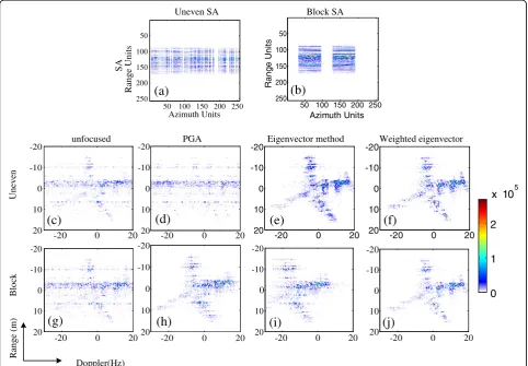
Figure 5SA-ISAR imaging results.(a) Uneven SA. (b) Block SA. (c) Imaging results without autofocusing method for uneven SA data. (d) Uneven SA-ISAR imaging with PGA. (e) Uneven SA-ISAR imaging with eigenvector method. (f) Uneven SA-ISAR imaging with weighted eigenvector method. (g) Imaging results without autofocusing method for block SA data. (h) Block SA-ISAR imaging with PGA. (i) Block SA-ISAR imaging with eigenvector method. (j) Block SA-ISAR imaging with weighted eigenvector method.

Table 1 Mean square error between true phase error and estimated error

PGA Eigenvector Weighted eigenvector

MSE¼ 1 K

XK

k¼1

u kð Þ−u

j j2_{; ð}

18Þ

where K is meant by the total number of Monte Carlo experiments under each generated SNR, u(k) represents the entropy value of the SA-ISAR imagery in thekth ex-periment, and u is the average entropy value of total in-dependent experiments under certain SNR.

4.2.2. Performance under SA cases

In this sub-section, random Gaussian phase error is ap-plied to defocus the dataset, and 128 pulses are extracted from the degraded dataset as SA samples. The SAs are il-lustrated in Figure 5a,b, respectively. The under-sampling processes are done in two ways, unevenly under-sampling and block under-sampling. Uneven SA is a general SA case, in which the missing data can occur at an arbitrary sampling index, and block SA is a familiar SA pattern in multiple-target observation with a single radar system. In this SA pattern, discontinuous blocks constitute the SA data, with each block having no missing samples.

Firstly, the sparsity-driven SA-ISAR imaging method is implemented to the range-compressed data without any autofocus methods. The results are presented in Figure 5c, g, respectively. The images are defocused in both SA cases. To autofocus the SA data, three methods (PGA, eigen-vector method, and weighted eigeneigen-vector method) are conducted. The imaging results manifest that the weighted eigenvector method achieves well-focused results under both SA patterns, as shown in Figure 5. However, the eigenvector method is only adaptable for the unevenly SA case, while the PGA is not suitable for both SA cases. Therefore, we conclude our method is suitable for auto-focusing data with different SA patterns, which is an extra-ordinary superiority to autofocusing methods available.

For quantitative comparison, the square error criterion given in [13] is adopted. Square error is computed according to (16) with the solutions listed in Table 1. Apparently, the weighted eigenvector has the smallest square errors in both SA patterns, which accords with the imaging results.

5. Conclusions

Based on the traditional eigenvector method, a weighted method is proposed. After comparing with traditional autofocus methods, such as PGA in conventional ISAR, it has been proven that the proposed method can achieve a well-focused SA-ISAR image, especially under low SNR conditions. With respect to the case that center shifting is not suitable for the SA-ISAR, zeropadding and iteration are implemented to eliminate discrete Doppler shift. Finally, the experimental results of real ac-quired data have testified that the proposed method is

capable to correcting phase error for SA-ISAR data with any pattern, whether block sparse-sampled or unevenly sparse-sampled data sets.

Competing interests

The authors declare that they have no competing interests.

Acknowledgments

The authors thank the anonymous reviewers for their valuable comments to improve the paper quality. This study was supported by the National Natural Science Foundation of China under grant nos. 61222108, JJ0200122201, and 61179010 and by the Fundamental Research Funds for the Central Universities under grants K5051302001 and K5051302038.

Received: 6 May 2012 Accepted: 1 April 2013 Published: 29 April 2013

References

1. L Zhang, M Xing, C Qiu, J Li, Z Bao, Achieving higher resolution ISAR imaging with limited pulses via compressed sampling. IEEE GRSL.6(3), 567–571 (2009) 2. H Joachim, G Ender, On compressive sensing applied to radar. IEEE Trans.

SP.90(5), 1402–1414 (2010)

3. L Zhang, Z Qiao, M Xing, J Sheng, R Guo, Z Bao, High resolution ISAR imaging by exploiting sparse apertures. IEEE Trans. Ant. Pro.60(2), 997–1008 (2012) 4. L Zhang, MD Xing, CW Qiu, J Li, J Sheng, Y Li, Z Bao, Resolution

enhancement for inversed synthetic aperture radar imaging under low SNR via improved compressive sensing. IEEE Trans. GRS.48(10), 3824–3838 (2010)

5. SD Babacan, R Molina, AK Katsaggelos, Bayesian compressive sensing using Laplace priors. IEEE Trans. IP.19(1), 53–63 (2010)

6. JA Tropp, AC Gilbert, Signal recovery from random measurements via orthogonal matching pursuit. IEEE Trans. IT.53(12), 4655–4666 (2007) 7. J Capon, High resolution frequency-wavenumber spectrum analysis. Proc.

IEEE.57, 1408–1418 (1969)

8. J Li, P Stocia, An adaptive filtering approach to spectral estimation and SAR imaging. IEEE Trans. Signal Process44(6), 1469–1484 (1996)

9. J Wang, D Kasilingam, Global range alignment for ISAR. IEEE Trans. Aerosp. Syst.39(1), 351–357 (2003)

10. T Sauer, A Schroth, Robust range alignment algorithm via Hough transform in an ISAR imaging system. IEEE Trans. Aerosp. Electron. Syst.31(3), 1173–1177 (1995)

11. D Zhu, L Wang, Y Yu, Q Tao, Z Zhu, Robust ISAR range alignment via minimizing the entropy of the average range profile. IEEE. Geosci. Remote Sens. Lett.6(2), 204–208 (2009)

12. DE Wahl, PH Eichel, DC Ghiglia, CV Jakowatz, Phase gradient autofocus—a robust tool for high resolution SAR phase correction. IEEE Trans. Aerosp. Electron. Syst.30(3), 827–834 (1994)

13. W Ye, TS Yeo, Z Bao, Weighted least-square estimation of phase errors for SAR/ ISAR autofocus. IEEE Trans. Geosci. Remote Sens.37(5), 2488–2494 (1999) 14. CV Jakowatz Jr., DE Wahl, Eigenvector method for maximum-likelihood

estimation of phase errors in synthetic-aperture-radar imagery. J. Optical Soc. Am.10(12), 2539–2546 (1993)

15. D Zhu, X Yu, Z Zhu, Algorithms for compressed ISAR autofocusing, in Proceedings of the 2011 IEEE CIE International Conference on Radar. Chengdu 24–27, 533–536 (Oct 2011)

16. MA Win, JH Winters, Analysis of hybrid selection/maximal-ratio combining in Rayleigh fading. IEEE Trans. Communications47(12), 1773–1776 (1999) 17. N Kong, LB Milstein, Average SNR of a generalized diversity selection

combining scheme. IEEE. Communication Letters3(3), 57–60 (1999) 18. J Wang, X Liu, Z Zhou, Minimum-entropy phase adjustment for ISAR. IEE.

Proc. Radar Sonar Navig.15(4), 203–209 (2004)

doi:10.1186/1687-6180-2013-92