A distributed approach to precoder selection using factor graphs for wireless communication networks

(1)

R E S E A R C H

Open Access

A distributed approach to precoder selection

using factor graphs for wireless

communication networks

Igor M Guerreiro

1*

, Dennis Hui

2

and Charles C Cavalcante

1

Abstract

This paper addresses distributed parameter coordination methods for wireless communication systems. This proposes a method based on a message-passing algorithm, namely min-sum algorithm, on factor graphs for the application of precoder selection. Two particular examples of precoder selection are considered: transmit antenna selection and beam selection. Evaluations on the potential of such an approach in a wireless communication network are provided, and its performance and convergence properties are compared with those of a baseline selﬁsh/greedy approach. Simulation results for the precoder selection examples are presented and discussed, which show that the

graph-based technique generally obtains gain in sum rate over the greedy approach at the cost of a larger message size. Besides, the proposed method usually reaches the global optima in an eﬃcient manner. Methods of improving the rate of convergence of the graph-based distributed coordination technique and reducing its associated message size are therefore important topics for wireless communication networks.

Keywords: Distributed optimization, Message-passing algorithm, Factor graphs, Precoder selection

Introduction

In a cellular network, there are many occasions in which each cell needs to set a parameter value, such as reference signal, transmit power, beam direction, or scheduled user, in such a way that the setting is preferably in a compatible way with the settings of the neighboring cells in order to achieve a certain notion of optimality, such as maximiz-ing the average system or user throughput, of the entire network [1,2]. The choice made by one cell on a local parameter often affects the interference level experienced by its immediate neighbors and hence their respective choices made on their local parameters, which in turn would influence the choices made by their neighbors’ neighbors. The simplest example is perhaps the classical frequency reuse problem [3] where the frequency band in which each cell transmits or receives is preferably differ-ent from those of its immediate neighboring cells to avoid mutual interference [4].

*Correspondence: [email protected]

1Wireless Telecommunication Research Group (GTEL), Universidade Federal do Cear´a (UFC), Fortaleza 60455-760, Brazil

Full list of author information is available at the end of the article

In some cases, such as the frequency reuse problem, the parameter is of relatively static nature and can be optimally planned and set before the network deploy-ment. However, in other cases, such as the transmit power control or antenna/beam selection problems, the param-eter is more dynamic and requires coordination to be continually performed. Therefore, a systematic method-ology for coordinating the choices of any parameters across the network is desired. Moreover, in order to facil-itate ﬂexible, dense deployment of small base stations in future cellular networks, there is also an increased interest in methods of performing the coordination of parameters among neighboring cells in an autonomous and distributed fashion without a central controller, as any unplanned addition (or removal) of base stations can sub-stantially alter the system topology and thus the preferred settings.

Factor graph and the associated sum-product algorithm have been widely used in probabilistic modeling of the relationship among interdependent (random) variables or parameters. There are numerous successful applica-tions [5] including, most notably, various fast-converging algorithms for decoding low-density parity check codes

(2)

and turbo codes, generalized Kalman filtering, fast Fourier transform, etc. One classic example motivated the most: the prisoner’s dilemma [6]. In a few words, the two pris-oners find an equilibrium point if both greedily betray. However, this is not a good solution because they can individually decrease their sentences if both of them stay silent, which is the best solution, and it is reached only if there is a sort of communication or centralization. In this context, the graph-based approach reaches the opti-mal solution by applying the message-passing algorithm. Similar (but different) applications of factor graphs have also been recently proposed for the problem of fast beam coordination among base stations in [7-10]. The basic idea in those works is to model the relationship between the local parameters to be coordinated among different communication nodes of a network and their respective performance metrics or costs using a factor graph [5]. In [7,8], the belief propagation algorithm is adopted to solve the downlink transmit beamforming problem in a multicell multiple-input-multiple-output (MIMO) system considering a one-dimensional cellular model. Moreover, in [9,10] some message-passing algorithms (including the sum-product algorithm) are deployed to coordinate parameters of downlink beamforming in a distributed manner in a multicell single-input-single-output system.

In this work, we propose a method founded on the min-sum algorithm on factor graphs for the application of precoder selection (i.e., transmit antenna selection [11] and beam selection) in a distributed manner. Based on factor graphs, a variant of the sum-product algorithm [5], namely the min-sum algorithm [12], can then be applied in order for all nodes, through iterative message passing with their respective neighbor nodes, to decide upon the best set of local parameters that can collectively maxi-mize a global performance metric across the network. The algorithm allows each communication node to be indeci-sive of its own decision until suﬃcient information about how its decision would aﬀect the overall network perfor-mance is accumulated. The perforperfor-mance of such a graph-based method along with other distributed methods, e.g., game-theoretic approach [13], for coordination of dis-crete parameters in a wireless communication network is evaluated.

Problem description

Consider a communication network withN

communica-tion nodes. A communicacommunica-tion node described here may represent any communication device in general in a wire-less communication network, for example, a base-station (BS), an access node, or a user equipment (UE) in a cellular communication system. Letpi, fori=1, 2,. . .,N, denote a discrete parameter (or a vector of two or more discrete parameters) of theith communication node, whose value is drawn from a ﬁnite setPi of |Pi| possible parameter

values for that node, where|Pi|denotes the cardinality of Pi, and let

p≡p1 p2 · · · pNT

be a vector collecting all the parameters in the network, where

pi∈Pi, i=1, 2,. . .,N.

Figure 1 shows a hexagon layout with N = 7

com-munication nodes where the set Pi = {1, 2, 3}, for

i = 1, 2,. . ., 7. Examples of discrete parameters are a precoding matrix index (PMI), which is largely used in 3GPP long-term evolution (LTE) systems and beyond to select precoding matrices [13,14] to maximize the net-work throughput, and an index to a frequency band in a frequency reuse planning to minimize the number of collisions in frequency bands, just to name a few.

Each nodeiis associated with a listNiof proper neigh-bor nodes (i.e., excluding nodei) whose choices of param-eter values can aﬀect the local performance of nodei. For convenience, also let

Ai≡Ni∪ {i}

denote the ‘inclusive’ neighbor list or just the neighbor list of nodei. Letp_Aidenote the vector of those parameters of

nodes inAi, with its ordering of parameters determined by the sorted indices in Ai. Associated with each node

i is a performance metric or cost, denoted byMi

pAi

, which is a function of those parameters in the neighbor listAiof nodei. Each nodeiis assumed to be capable of communicating with all nodes inAi.

(3)

Our goal is for each node i to ﬁnd, in a distributed fashion, its own optimal parameterp∗_i, which is the cor-responding component of the optimal global parameter vector p∗ that minimizes the total (global) performance metric given by

The problem of coordinating parameters can be solved adopting basically two types of solutions: (1) centralized approach, which yields the optimal global parameter vec-tor, and (2) distributed approaches, which on one hand often provide suboptimal solutions through greedy tech-niques such as non-cooperative games, but on the other hand can provide near-optimal solutions by using a factor graph.

Centralized solution

Conceptually, the simplest approach to the optimization problem described above is to solve it jointly at a central location by direct computing

pC≡

which is an optimal solution to the problem by deﬁnition. A major issue of this approach is its huge computational complexity for large network size N, as the complexity grows exponentially as the number of communication nodes increases, along with the inherent high signaling load (backhaul traﬃc) between the communication nodes and a central processing unit.

The computational complexity of the centralized solu-tion is indeed very high. The minimum (or maximum) value of a cost (utility) function is usually found through-out all the combinations of the discrete parameters. The total number of combinations of parameterscis given by

c= must be done to ﬁnd the optimal value, which might be computationally prohibitive. Alternatively, the centralized technique may be replaced with the standard alternating-coordinate optimization technique for dense networks. Such an approach starts with an arbitrary choice of p

and iteratively optimizes each element (or a particular set of elements) ofpone at a time while holding others ﬁxed. Its convergence to the globally optimum result can be guaranteed under under some conditions, e.g., convex utility/cost function.

Selﬁsh/greedy solution

Another approach to the optimization problem above is for each communication node to selﬁshly set its own parameter to optimize its own local performance based on the most recent choices made and given by its neighbors. In this approach, the complexity of each node grows only linearly with the cardinality of the set of parametersPi since only the parameters of the node itself are considered in the optimization at the node. More precisely, in this approach, the local parameterpi at each communication node is iteratively chosen as

p(_Sn+_,_i 1)≡arg min of pi made at iteration n + 1 using this selﬁsh/greedy approach, andp(_Sn_,_N)

idenotes the vector of those parameter

choices made by nodes inNiat thenth iteration. In turn, the parameterp(_Sn_,_i)at each node is exchanged to its neigh-boring nodes so that every node obtains its parameter vectorp(_Sn_,_N)

ito compute its next parameterp (n+1)

S,i . From a game-theoretic perspective, the greedy solu-tion may be seen as a non-cooperative game [6]. In this sense, the (greedy) game solution can be defined as a pure-strategy Nash equilibrium (NE). In a few words, a NE is established if each player (i.e., each communication node) has chosen an action (i.e., a local parameterpS,i) and no one can benefit from changing its action unilaterally while the others keep theirs unmodified. Therefore, an action tuplep

The superscriptdenotes that the underlying parameter leads to a NE. The inequality above is a convenient form for representing a NE.

Graph-based solution

In the following, we describe another approach to the problem of minimizing the global metric in (1) by mod-eling the communication nodes and the associated local performance metrics using a factor graph. A factor graph is a bipartite graph consisting of a set of variable nodes and a set of factor nodes. Each variable node represents a vari-able and can only be connected to a factor node (but not another variable node) through an edge, while each factor node represents a factor which is a function of some of the variables. A factor node is connected to a variable node if and only if the corresponding function represented by the factor node depends on that variable.

(4)

Figure 2Factor graph model for a communication network with local parameters and local performance measures.

multivariate function into several local functions. In our problem at hand, the global performance metric M(p) is factorized into a sum of N local performance met-rics Mi

p_Ai

, which is described in (1). Speciﬁcally, for the problem formulated above, we associate each vari-able node with the parameterpiof a communication node and each factor node with its local performance metric

Mi

p_Ai

. Accordingly, we label a variable node corre-sponding topi asv(pi)and a factor node corresponding toMi

p_Ai

asv(Mi). An edge connecting a factor node

v(Mi)with a variable nodev(pk)exists if and only ifk ∈ Ai. For example, Figure 2 shows a hexagon layout of seven communication nodes, each associated with a factor node representing the local performance metricMi

pAi

and a variable node representing the local parameterpi. The factor node associated with the local performance metric

Mi

pAi

of communication nodeiis connected through edges to the respective variable nodes associated with its

own local parameterpi and those parameters{pi}i∈Ni of

its neighbors upon which the metric Mi

pAi

depends. For clarity, we use a diﬀerent color to represent diﬀer-ent communication nodes and the corresponding edges connecting their respective factor nodes with the relevant variable nodes.

The graph in Figure 2 can be also re-organized as in Figure 3, which clearly shows the bipartite property of the graph with factor nodes connected only to variable nodes through the respective edges. A message-passing algorithm, such as the sum-product algorithm, can then be executed on such a graph. Speciﬁc messages are com-puted and passed along each edge of the graph. Those messages that are passed on edges connecting factor and variable nodes of diﬀerent colors correspond to informa-tion exchange between two neighboring communicainforma-tion nodes, while those messages that are passed on edges that connect nodes of the same color represent inter-nal communications within each communication node. Each message depends only on the variable whose associ-ated variable node is a vertex of the edge over which the message is passed along. More precisely, each message is simply a table of values with each entry corresponding to one of the possible values of the variable, as described in detail in the following.

The graph-based distributed parameter coordination algorithm

In this section, we describe the algorithm associated with the proposed distributed solution for the problem of parameter coordination. The sum-product algorithm [5] can be applied whenever the variables and functions asso-ciated with the factor graph are deﬁned on a commutative semi-ring whose elements satisfy the distributive law. For our problem at hand, we apply the variant of sum-product algorithm that is based on the min-sum commutative semi-ring [12]. Recall that a semi-ring is a mathemat-ical structure (e.g., a set) equivalent to a ring without an additive inverse. In a general way, the binary oper-ations addition and multiplication can be replaced with others as long as the distributed law still holds. In this sense, a min-sum semi-ring simply replaces the addition operation with the minimum operation and the multipli-cation operation with the addition operation. In this case,

(5)

the sum-product algorithm is also called the min-sum algorithm.

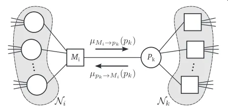
More speciﬁcally, letμMi→pk(pk) denote the message

to be passed from a factor node v(Mi) to a variable nodev(pk), and letμpk→Mi(pk)denote the message to be

passed from the variable nodev(pk) to the factor node

v(Mi). Figure 4 shows the two kinds of messages pass-ing on in a fragment of a factor graph. The min-sum algorithm, when applied to our problem at hand, sim-ply iterates between the following two kinds of message computations and exchanges:

1. Factor node to variable node:

μMi→pk(pk)=_pmin

where the notation\{k}means that the underlying operator is performed over all associated variables except to variablek. To prevent messages from increasing endlessly, the messages are normalized to have zero mean.

2. Variable node to factor node:

μpk→Mi(pk)=

j∈Ak\{i}

μMj→pk(pk), (6)

which aggregates all the incoming messages at variable nodev(pk)except to the one from factor nodev(Mi).

Here, an ideal error-free message pass is considered. The algorithm may begin with each factor node v(Mi) computing outgoing message μ_M_i_→p_k(pk) to v(pk) for

each k ∈ Ai using (5) with all incoming messages

μpk→Mi(pk)from connected variable nodes initialized to

unit messages, that is, messages with entries equal to zero for the problem at hand. It is worth mentioning that the initialization with unit messages may lead nodes to compute and propagate messages with equal entries. In

Figure 4A factor-graph fragment, showing the message pass between factor nodeMiand variable nodepk.

such situation, nodes are not capable of iteratively ﬁnd-ing the best parameters as all the entries return the same cost. To circumvent this, the initial incoming messages μpk→Mi(pk)can be initialized to random values close to messages increasing endlessly. The parameter for commu-nication nodeiis determined at its variable nodev(pi)by

p∗_i =arg min

The algorithm then iterates until a stopping criterion is reached, either a predetermined maximum number of iterationλor when the set of parameters computed in (7) converges to a ﬁxed state, that is, the updated messages are equal to the previous computed messages, or equivalently,

p(_in+1)=p_i(n), ∀i=1, 2,. . .,N, (8)

wherenis an iteration index such thatn≤λ.

Note that both messages computed in (5) and (6) depend only on the value ofpk. Sincepk ∈ Pk andPk is assumed to be discrete and ﬁnite, each of the messages can be represented by a table of|Pk|entries.

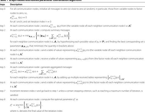
In particular, the computation in (6) is just adding up the corresponding entries of multiple tables of the same size together. We summarize the proposed graph-based distributed coordination method from each communica-tion node’s perspective in Table 1. Note that to reduce computational complexity, the minimization operation in (5) in step 2 can be computed through the standard alternating-coordinate optimization technique, although its convergence may not be guaranteed in this case.

When the factor graph contains no cycle (i.e., a closed path in the graph), it can be shown [5] that the message-passing algorithm described above will yield the exact optimal solution that optimizes (1) in a single iteration. However, when it contains cycles, the algorithm has no natural termination and the messages pass multiple times on the edges of the factor graph in an iterative manner. In this case, the algorithm typically yields good approxima-tions to the true optimal solution [5].

(6)

Table 1 Graph-based distributed parameter coordination algorithm

Steps Description

Step 0 For all communication nodes, initialize all messages to zero (or close to zero at random), in particular, those from variable nodes to factor

nodes to zero, i.e.,

μ(_p0_k)_→_M_i (pk)=0

for alliandk, and set iteration indexn=0

Step 1 At each communication nodei, receiveμ(_pn)

k→Mi (pk)from (the variable node of) each neighbor communication nodek∈Ni

Step 2 At each communication nodei, compute summary messages

μ(_Mn_i+_→1)_p_k(pk)=minpAi\{k}

MipAi

+

j∈Ai\{k}

μ(_pn_j_→) _M_ipj

,

for each neighbor communication nodek∈Ai, by hypothesizing each possible value ofpkinPkand ﬁnding the best corresponding set of

parametersp_A_i_\{k}that minimizes the quantity in brackets above Step 3 At each communication nodei, send a table of values representingμ(_Mn+1)

i→pk(pk)to (the variable node of) each neighbor communication

nodek∈Ni

Step 4 At each communication nodei, receive a table of values representingμM_k→pi(pi)from (the factor node of) each neighbor communication

nodek_∈_Ni

Step 5 At each communication nodei, generate aggregated messages

μ(_pn_i_→+1_M)_k(pi)=μ(_Mn_i+_→1_p)_i(pi)+ j∈Ni\{k}

μ(_Mn_j+_→1)_p_i(pi)

for each neighbor communication nodek∈Aiby adding up multiple received tables representing

μ(_Mn+1) j→pi(pi)

j∈Ni

Step 6 At each communication nodei, send a table of values representingμ(_pn_i_→+1_M)

k(pi)to (the factor node of) each neighbor communication node k∈Ni

Step 7 Increment iteration indexnand go back to step 1 unless a certain stopping criterion, such as reaching a maximum number of iteration, is

satisﬁed

Step 8 At each communication nodei, compute the optimal parameterp∗_i as

p∗_i =arg min

pi

j∈Ai μ(nf)

Mj→pi(pi)

,

wheren_fdenotes the ﬁnal value of the iteration index

random scheduling, which is discussed below, acts as a perturbation in the system.

Message-passing scheduling

Regarding cases with cyclic graphs, the iterative process described above must follow a message-passing sched-ule to compute approximations of the true marginal functions. That is, the message-passing schedule must describe the way nodes are activated and the way mes-sages are passed at each iteration. Note that the graph-based algorithm follows the message propagation rules previously described. In this work, two sorts of node scheduling based on the so-called ﬂooding schedule [15] were considered: (1) random scheduling (RS), where each node has a certain probability of being activated to partic-ipate in the message pass at each iteration, and (2) simul-taneous scheduling (SS), where all the nodes participate in the message pass at the same time at each iteration:

1. Random scheduling: In this scheduling mode, each node has two possibilities (which is similar to a ‘coin

ﬂipping’) at each iteration of the message-passing process: being either active or inactive. LetPactivebe the probability of being active, i.e., the chance of passing/receiving messages, during the iterative message-passing process. Thus, every node hasPactive % chance of being active at each iteration. If a node is inactive in a particular iteration, that node neither receives nor passes messages on its associated edges. That is, the messages associated with that node are not updated.

2. Simultaneous scheduling: In this scheduling mode, all the nodes pass/receive messages to/from their neighboring nodes, which is equivalent to set

Pactive=1in the mode RS, i.e., 100% of the nodes active during the whole message-passing process.

(7)

On the other hand, the mode SS can reach a potential convergence point in a faster manner since all the nodes exchange messages. Thus, the choice of the message-passing scheduling mode might depend on the network demand, such as latency and backhaul traﬃc. Moreover, the parameterPactivemay be optimized in order to either decrease the signaling load or speed up the convergence.

In the following, the application in which the proposed algorithm is evaluated as well as its associated parameters and performance metrics is presented.

Precoder selection problem

In this section, we discuss the parameter coordination problem, i.e., precoder selection, modeled by (1) in the context of wireless communications. Each parameter pi may represent a PMI for BSi in the downlink (or UEi

in the uplink) in a cellular network, indicating which pre-coder from a predetermined setPiof precoders or beam-forming weights that BS (or UE)ishould use at a certain radio resource block to transmit signals. In practical sys-tems, different UEs may be scheduled, and thus, different precoders may be used at different radio resource blocks. In this case, the coordination of precoders may be per-formed independently for each individual radio resource block.

Consider a multicell MIMO system in the downlink in which each BS has Nt available transmit antennas and each item of UE hasNrreceive antennas. For convenience, each item of UE is simply referred to as a UE. The BSi

transmits precoded and spatially multiplexed vectorxito its associated UEi. The vectorxiis deﬁned as

xi= spatially multiplexed symbol vector, andW(pi) ∈ W is theNt×Nsprecoding matrix speciﬁed by the parameter

pi. Examples of setW can be a LTE precoder codebook, a ﬁxed beamforming weight codebook, and a transmit antenna selection (TAS) codebook. In general,W is the set of all precoding matrices available for every communi-cation node in the network. In order to index the elements ofW, assume an index setI, which is equivalent toPi,

for all the communication nodes. Then, a bijective function

f:Pi↔W (10)

maps the elements ofPionto the elements ofWproperly.

This work focuses on two particular examples of pre-coding matrix W: (1) TAS precoders and (2) discrete Fourier transform (DFT)-matrix-based precoders:

1. Transmit antenna selection: Let each element ofW be anNt×Nssubmatrix of an identity matrixINt.

That is, the unique non-null entry of each column of this submatrix selects a transmit antenna. For example, forNt=3andNs=2,

where each matrix inWis a particularWindexed by

pi∈Pi, according to (9) and (10). In other words, each matrixWselects two antennas out of three, where the ﬁrst matrix selects antennas 1 and 2, the second matrix selects antennas 1 and 3, and ﬁnally the last matrix selects antennas 2 and 3.

2. Fixed-beam selection: Let each element ofWbe an

Nt×Nssubmatrix of theNt×NtDFT matrixF

logarithm andj is the imaginary unit. Basically, each matrixWchanges the relative phase and direction of the vectorsto be transmitted. For instance, for

Nt=3andNs=2,

where each matrix inW, similar to the TAS case, is a particularWindexed bypi∈Pi, according to (9) and (10). In this example, there are three diﬀerent beams to be selected, each one with a diﬀerent combination of phase and direction.

The sampled incoming signal vector at the receiveriis given as being

yi =√giiHiixi+

j∈Ni

gjiHjixj+vi, (13)

whereHji denotes the MIMO channel response from BS

(8)

1

2

3 1

2 0

0.5 1 1.5 2 2.5 3 3.5

Tx eigenmodes Coupling Matrix

Rx eigenmodes

Figure 5Estimated power coupling matrix of2×3MIMO channel matrices.

a gain that corresponds to the path loss of each signal, here modeled in a simpliﬁed way as being

gji=

1

dji

α

, (14)

where the constant α refers to the path loss exponent anddjiis the distance between the transmitterjand the receiveri. The second term on the right-hand side refers to the interference caused by the neighboring communi-cation nodes. For each transmitter, the average transmit power is constant and given by

E!xi2

" = 1

Ns

trWWH=PT, (15)

where PT is the average transmitted power in units of energy per signaling period. Also, the symbols are assumed to be uncorrelated, which means thatE!sisHi

" =

INs.

In both cases, the local performance metric Mi

p_Ai

may represent the negative of the data throughput [16,17] of the cell corresponding to BSimeasured by

Mi

pAi

= −log det

#

I+ |gii|R−_i1HiiW(pi)W(pi)HHHii

$

,

(16)

whereRi, deﬁned herein as

RiRvi+

j∈Ni

|gji|HjiW(pj)W(pj)HHHji, (17)

denotes the covariance matrix of the noise plus interfer-ence experiinterfer-enced by the UE served by BSiin the down-link given thatRvi is the covariance matrix of the noise

vectorvi.

The global performance metric is simply the total data throughput in the network. Hence, the goal here is to

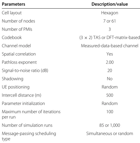
Table 2 Parameters of simulation

Parameters Description/value

Cell layout Hexagon

Number of nodes 7 or 61

Number of PMIs 3

Codebook (3_×2) TAS or DFT-matrix-based

Channel model Measured-data-based channel

Spatial correlation Yes

Pathloss exponent 2.00

Signal-to-noise ratio (dB) 20

Shadowing No

UE positioning Random

Intercell distance (m) 500

Parameter initialization Random

Maximum number of iterations per run

100

Number of simulation runs 85 or 1,000

Message-passing scheduling type

(9)

15 20 25 30 35 40 45 50 0

0.1 0.2 0.3 0.4 0.5 0.6 0.7 0.8 0.9 1

Sum Rate [bits/channel use]

Cumulative Distribution

Centralized Graph, SS Graph, RS90% Graph, RS70% Graph, RS30% Greedy, SS Greedy, RS90% Greedy, RS70% Greedy, RS30% Random

Figure 6Performance analysis of graph-based technique for TAS problem in terms of sum rate in seven-node network.

employ a distributed algorithm for the BS to negotiate their choices of downlink precoding matrices with their respective neighbors so that the total data throughput in the network is maximized.

The channel response includes both a fast fading com-ponent and a path loss comcom-ponent, the latter determined by the distance between the corresponding BS and UE, according to (14). A basic system model is therefore needed to compute the relative distances between BS and UEs for each random drop of UEs in the cell grid considering ﬁxed BSs’ positioning. For convenience, the log-normal shadowing has not been modeled in this work. To obtain more realistic results, each MIMO chan-nel response was drawn from a data setD of measured channel matrices acquired by Ericsson Research during measurement campaigns made in Kista neighborhood in Stockholm, Sweden. The measurement campaigns were performed using a single BS placed on the roof of a build-ing and a UE mounted inside a van at a convenient drivbuild-ing speed (see more details in [18,19]). A total of 324,000 samples of 2×3 channel matrices measured along a par-ticular route of Kista compound the setD. For the sake of

removing any ‘original’ large-scale fading eﬀect, each entry of the channel matrices was previously transformed into a zero-mean and unity-variance variable, such that

Hji_k_,_l=

Dji_k_,_l−μD

σD , Dji∈D, k=1

. . .2, l=1. . .3,

(18)

whereDji, randomly picked up from setD, is associated with receiverjand transmitteri,μ_Dandσ_D2are the mean and the variance of the entries of the matrices in D, respectively, andHji is the transformed MIMO channel matrix also associated with receiver j and transmitter

i. The indices k and l index the element (k,l) of both matrices Dji and Hji. Then, the path loss modeled by the parameters gji is in turn inserted to the matrix Hji according to (13). It is worth noting that each element ofD is randomly chosen only once so that each pair of receiver and transmitter has a diﬀerent channel matrix. Particularly, the resulting channel matrices are charac-terized by the presence of a number of eigenmodes less than 2. Such a feature is observed in the estimated power

Table 3 Percent gain in sum rate for the TAS problem in a seven-node network

% Gain in sum rate over greedy Message-passing scheduling

Simultaneous 90% Random 60% Random 30% Random

(10)

1 2 3 4 5 6 7 8 9 10 0

0.1 0.2 0.3 0.4 0.5 0.6 0.7 0.8 0.9 1

Number of Iterations until Convergence

Graph, SS Graph, RS90% Graph, RS70% Graph, RS30% Greedy, SS Greedy, RS90% Greedy, RS70% Greedy, RS30%

Figure 7Convergence speed of graph-based technique against greedy technique for TAS problem in seven-node network.

coupling matrix[20] of resulting MIMO channel matri-ces, which is shown in Figure 5. The matrixshows the spatial arrangement of scattering objects between the transmitter and the receiver, where its columns refer to the transmit eigenmodes and the rows the receive eigen-modes. This matrix characterizes the entire data set D. Consequently, as all the pairs of receiver and transmitter draw their channel matrices from D, they observe the same spatial correlation. The motivation to use such a channel model is to provide a suitable scenario for the beam selection technique, which usually beneﬁts from the characteristics of spatially correlated channel matrices.

Next, simulation results of the application of the pro-posed method in the precoder selection problems are shown and discussed.

Simulation results

In this section, the global performance metric presented in (16) in the precoder selection problem is investigated in order to evaluate how it behaves statistically in terms

of cumulative distribution curves CDFs. Both examples of precoding selection, TAS and beam selection, are com-pared with the centralized solution, which is optimal by definition; the greedy solution, which is expected to pro-vide a suboptimal result; and a lower bound propro-vided by the random choice of the precoding matrix, kept con-stant during the simulation run, at each node. Moreover, the convergence speed, which is inversely proportional to the average number of iterations until convergence per simulation run, of both distributed approaches is qualita-tively assessed in terms of CDF curves for only the cases where the underlying algorithm converges, following (4) and (8). Additionally, the convergence rate, defined as the ratio of the number of runs where the underlying algo-rithm converges to the total number of simulation runs, is shown for both distributed techniques. Both distributed algorithms are evaluated considering the different types of message-passing scheduling.

In order to evaluate the scalability of the proposed algo-rithm, a hexagon layout withN=7 orN=61 cells and a

Table 4 Convergence rate for the TAS problem in a seven-node network

Technique Message-passing scheduling

SS RS,Pactive=0.9 RS,Pactive=0.7 RS,Pactive=0.3

Graph-based 0.980 0.985 0.993 1

(11)

150 160 170 180 190 200 210 220 230 240 0

0.1 0.2 0.3 0.4 0.5 0.6 0.7 0.8 0.9 1

Sum Rate [bits/channel use]

Alt. Coordinate Graph, SS Graph, RS90% Graph, RS70% Graph, RS30% Greedy, SS Greedy, RS90% Greedy, RS70% Greedy, RS30% Random

Figure 8Performance analysis of graph-based technique for TAS problem in terms of sum rate in 61-node network.

single communication node in each cell was adopted. It is worth noting that for the case ofN = 61, the centralized technique was replaced with the alternating-coordinate technique. In this case, the set of parameters of a cer-tain neighborhood are coordinated while holding others ﬁxed. The precoding matrix codebooks deﬁned in (11) and (12) were used as the parameter set for TAS and beam selection, respectively. As for the MIMO setup, each transmitter hasNt = 3 available transmit antennas and

Ns= 2 data streams to be transmitted, and each receiver hasNr = 2 receive antennas. To obtain more realistic results, each MIMO channel response was drawn from a set containing 324,000 2× 3 channel matrices, accord-ing to (18). The parameter initialization is at random, i.e., nodes pick one of the PMIs randomly at the beginning of each simulation run in the greedy technique. In the graph-based approach, the initial messages deﬁned in (6) are equal to zero. The maximum number of iterationsλ in each simulation run is 100. Finally, a total of 1,000 runs were conducted for statistical purposes for the seven-node network case. Due to the fact that the number of channel

data samples available is limited, a total of only 85 runs were conducted for the 61-node network case. It is worth mentioning that the channel responses were kept con-stant during theλiterations. These simulation parameters above were adopted for both simultaneous and random message-passing schedulers. As for random scheduling, the parameterPactivewas set to 90%, 70%, or 30%. Table 2 lists the simulation parameters.

Example 1: transmit antenna selection

For the TAS example, the number of radio frequency chains is 2. Consequently, the parameters to be coordi-nated are three PMIs for all the cells. Such parameters index the elements of the codebook in (11). Next, simula-tion results considering a network with seven cells, each one with a communication node, are presented.

TAS andN =7nodes

The graph-based technique appears not to be aﬀected by the diﬀerent types of message-passing scheduling in terms of sum rate. Figure 6 shows that the proposed method

Table 5 Percent gain in sum rate for the TAS problem in a 61-node network

(12)

2 4 6 8 10 12 14 16 18 20 22 24 0

0.1 0.2 0.3 0.4 0.5 0.6 0.7 0.8 0.9 1

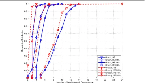
Figure 9Convergence speed of graph-based technique against greedy technique for TAS problem in 61-node network.

in all the scheduling modes provides approximately the same performance. The maximum achievable sum rate is about 49 bits per channel use, reached by the cen-tralized approach and also by the graph-based technique. From the curves in Figure 6, the graph-based technique approaches the optimal solution in all the simulation runs, reaching the global optimum in most of them. Clearly, the graph-based technique outperforms the greedy one.

The greedy technique is also not significantly affected by the different types of message-passing scheduling in terms of sum rate. According to Figure 6, the greedy technique with any of the scheduling modes reaches the sum rate value of 48 bits per channel use or less with 100% probabil-ity, while both the proposed and the centralized technique provide about 49 bits per channel use.

According to the results, the gain in sum rate obtained by the graph-based technique over the greedy one is largely independent of the type of scheduling. For instance, from the 50th CDF percentile, such a gain is about 2.4% for all the message-passing scheduling modes.

Table 3 shows the statistics above. Despite the small gain observed over the greedy, the proposed method provides a solution near (or equal to) the optima.

It is clear that the TAS with both greedy and graph-based solutions outperforms the random choice approach. However, the maximum gain obtained over the random choice is around 9%, which may be considered too small for a precoder selection technique.

With respect to convergence speed, the proposed method with random scheduling converges faster than that with simultaneous scheduling. Figure 7 shows that the higher the probability of being active, the higher the speed of convergence. The same behavior occurs for the greedy technique. However, it converges faster than the graph-based. Both greedy and graph-based techniques converged in ten iterations or less with 100% probability.

In terms of convergence rate, the proposed method has a diﬀerent rate for each message-passing scheduling mode. For instance, the graph-based technique with simultane-ous scheduling converges with 98% probability. Further,

Table 6 Convergence rate for the TAS problem in a 61-node network

SS RS,Pactive=0.9 RS,Pactive=0.7 RS,Pactive=0.3

Graph-based 0.882 0.905 0.941 1

(13)

10 20 30 40 50 60 0

0.1 0.2 0.3 0.4 0.5 0.6 0.7 0.8 0.9 1

Sum Rate [bits/channel use

Centralized Graph, SS Graph, RS90% Graph, RS70% Graph, RS30% Greedy, SS Greedy, RS90% Greedy, RS70% Greedy, RS30% Random

Figure 10Performance analysis of graph-based technique for beam selection problem in terms of sum rate in seven-node network.

the proposed method with random scheduling converges with 98.5% when Pactive = 0.9, 99.3% probability when

Pactive = 0.7, and 100% probability whenPactive = 0.3. Finally, the greedy technique with random scheduling converges with 100% probability, while it converges with 99.6% probability in the simultaneous scheduling mode. Table 4 shows all the statistics regarding convergence rate. Interestingly, even when the proposed method does not converge, it provides a near-optimal solution, as expected. In the following, simulation results considering a larger network withN=61 are presented.

TAS andN =61nodes

Increasing the network size to 61 nodes, the graph-based technique is still not aﬀected by the diﬀerent modes of message-passing scheduling in terms of sum rate. Accord-ingly, Figure 8 shows that all the scheduling modes make the proposed method to have approximately the same per-formance. For this network size, the centralized approach is properly replaced with the alternating-coordinate tech-nique, which provides the ‘best’ solution in this case.

It reaches a maximum sum rate of about 231 bits per channel use, followed by the graph-based technique. In Figure 8, the proposed method approaches the best solu-tion in all the simulasolu-tion runs (often reaching the best) and outperforms the greedy technique. Moreover, the proposed method appears to be scalable since it main-tains its good performance in larger networks. The greedy technique is also not significantly affected by the differ-ent types of message-passing scheduling, but as shown in Figure 8, the maximum achievable sum rate for such an approach is around 227 bits per channel use.

In general, the gain in sum rate obtained by the graph-based technique over the greedy one is largely indepen-dent of the scheduling mode in terms of sum rate. For instance, from the 50th CDF percentile, the gain is about 1.459% for all the scheduling modes. Again, the gain obtained over the random choice is too small, around 8%. Table 5 shows the statistics above.

As for convergence speed, the graph-based technique with simultaneous scheduling converges faster than that with random scheduling, as in the previous case. Figure 9

Table 7 Percent gain in sum rate for the beam selection problem in a seven-node network

(14)

0 5 10 15 0

0.1 0.2 0.3 0.4 0.5 0.6 0.7 0.8 0.9 1

Figure 11Convergence speed of graph-based technique against greedy technique for beam selection problem in seven-node network.

also shows that the higher the probability of node acti-vation, the higher the speed of convergence. Again, the greedy technique has the same behavior, but it converges faster than the graph-based technique. In Figure 9, both techniques converge in up to 24 iterations.

With regard to convergence rate, the graph-based tech-nique observes diﬀerent rates, which depends on the message-passing scheduling mode. For instance, such an approach with simultaneous scheduling converges with 88.2% probability. However, considering random schedul-ing, it converges with 90.5% probability whenPactive=0.9, with 94.1% probability whenPactive= 0.7, and with 100% whenPactive =0.3. Diﬀerently, the greedy technique con-verges with 100% probability in all the scheduling modes except in the simultaneous scheduling mode, where it converges with 96% probability. Table 6 shows all the statistics above regarding convergence rate.

Example 2: ﬁxed-beam selection

For the beam selection problem, the parameters to be coordinated are also three PMIs for all the cells. Such

parameters index the elements of the codebook in (12). Next, simulation results considering a network with seven cells, each one with a communication node, are presented.

Beam selection andN=7nodes

Similar to the previous example, the graph-based tech-nique appears not to be aﬀected by the diﬀerent modes of message-passing scheduling in terms of sum rate. In Figure 10, the proposed method has approximately the same performance in all the scheduling modes. The maxi-mum achievable sum rate is about 51 bits per channel use, reached by both the centralized and graph-based tech-niques. From the curves in Figure 10, the graph-based technique approaches the optimal solution in all the simu-lation runs, reaching the global optimum in most of them. Once more, the proposed method provides a near-optimal solution. As expected, the graph-based technique outper-forms the greedy and also the random choice with a large gain in sum rate.

The greedy technique is not aﬀected by the diﬀerent types of message-passing scheduling in terms of sum rate.

Table 8 Convergence rate for the beam selection problem in a seven-node network

Graph-based 0.906 0.919 0.959 1

(15)

160 180 200 220 240 260 0

0.1 0.2 0.3 0.4 0.5 0.6 0.7 0.8 0.9 1

Sum Rate [bits/channel use

Alt. Coordinate Graph, SS Graph, RS90% Graph, RS70% Graph, RS30% Greedy, SS Greedy, RS90% Greedy, RS70% Greedy, RS30% Random

Figure 12Performance analysis of graph-based technique for beam selection problem in terms of sum rate in 61-node network.

Still in Figure 10, the greedy technique with any of the scheduling modes reaches the sum rate value of 45 bits per channel use or less with 100% probability, while both the proposed and the centralized technique provide about 51 bits per channel use as aforementioned. Figure 10 also shows that the greedy technique poorly outperforms the random choice.

Based on the curves in Figure 10, the gain in sum rate obtained by the graph-based technique over the greedy is largely independent of the mode of scheduling. For instance, from the 50th CDF percentile, such a gain is around 24.7% for all the message-passing scheduling modes. Table 7 shows the statistics above. Dissimilarly to the previous example, the gain observed over the greedy and the random choice is signiﬁcantly large.

As for convergence speed, the proposed method tech-nique with random scheduling converges faster than that with simultaneous scheduling. Figure 11 shows that the higher the probability of being active, the higher the speed of convergence. Again, the greedy technique behaves the same way, i.e., converges faster than the graph-based

technique. Both the greedy and graph-based techniques converge in 15 iterations or less with 100% probability.

In terms of convergence rate, the graph-based technique has a diﬀerent rate for each message-passing schedul-ing mode adopted. For instance, the graph-based tech-nique with simultaneous scheduling converges with 90.6% probability. Further, the proposed method with random scheduling converges with 91.9% when Pactive = 0.9, 95.9% probability whenPactive = 0.7, and 100% proba-bility whenPactive = 0.3. On the other hand, the greedy technique converges with 100% probability with any of the message-passing scheduling types. Table 8 shows all the statistics regarding convergence rate. Once again, even when the proposed method does not converge, it provides a near-optimal solution, as expected.

Beam selection andN =61nodes

Considering a network size of 61 nodes, the graph-based technique is still not aﬀected by the diﬀerent modes of message-passing scheduling in terms of sum rate. Such a behavior is shown in Figure 12, where all the scheduling

Table 9 Percent gain in sum rate for the beam selection problem in a 61-node network

(16)

5 10 15 20 25 30 35 40 0

0.1 0.2 0.3 0.4 0.5 0.6 0.7 0.8 0.9 1

Figure 13Convergence speed of graph-based technique against greedy technique for beam selection problem in 61-node network.

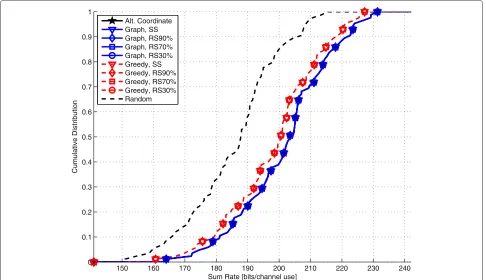
modes make the proposed method to have approximately the same performance. Properly, the centralized approach is replaced with the alternating-coordinate technique, which reaches a maximum sum rate of about 257 bits per channel use, followed by the graph-based technique. In Figure 12, the proposed method approaches the solution of the alternating-coordinate technique in all the simula-tion runs (often reaching that result) and outperforms the greedy technique. Thus, the proposed method maintains its good performance even in such a larger network. The greedy technique is not significantly affected by the differ-ent modes of message-passing scheduling, but Figure 12 shows that it achieves a lower maximum sum rate of 218 bits per channel use. Again, the random choice is greatly outperformed by the proposed technique.

As observed in all the examples above, the gain in sum rate obtained by the proposed method over the greedy technique is independent of scheduling mode in terms of sum rate. For example, from the 50th CDF percentile, the gain is around 21% for all the scheduling modes. Table 9 shows the statistics above.

In terms of convergence speed, the graph-based tech-nique with the simultaneous scheduling converges faster than that with random scheduling, as in all the previ-ous cases. For both the graph-based and greedy tech-niques, Figure 13 shows that the higher the probability of node activation, the higher the speed of convergence. In Figure 13, both techniques converge in up to 38 iterations. Nevertheless, the greedy technique converges faster than the graph-based.

As for convergence rate, the graph-based technique observes diﬀerent rates, which depends on the message-passing scheduling mode. However, in this example, the proposed method shows small convergence rates. For instance, the graph-based approach with simultaneous scheduling converges with 16.4% probability. Consider-ing random schedulConsider-ing, it converges with 22.3% proba-bility when Pactive = 0.9, with 22.3% probability when

Pactive = 0.7, and with 36.4% when Pactive = 0.3. On the contrary, the greedy technique converges with 100% probability in all the scheduling modes. Table 10 shows all the statistics above regarding convergence rate. The

Table 10 Convergence rate for the beam selection problem in a 61-node network

Graph-based 0.164 0.223 0.223 0.364

(17)

small number of simulation runs in this example may have led to those small rates, but despite those rates, the pro-posed method has a similar performance compared to the alternating-coordinate technique and also outperforms the greedy solution with large gain in sum rate.

Summary of the results

The small observed gain in the TAS problem is likely due to the choice of the particular precoder codebook of antenna selection. The selection of transmit antennas at a certain node seems not to signiﬁcantly aﬀect the selection made by the others and, consequently, poorly mitigates mutual interference observed by nodes. Therefore, even the simpler greedy solution may achieve a good result. Besides, the comparison of the TAS with the random choice shows that it does not have a great impact on the performance of the nodes since it provides gains in sum rate below 10%.

In the fixed-beam selection problem, the large observed gain is likely due to the use of directional beamforming precoding matrices. The selection of fixed beams at a cer-tain node seems to impact on the selection made by the others since it may directly avoid a node causing inter-ference to its neighbors. Thus, the graph-based technique can obtain a better solution than the greedy one based on the fact that the messages exchanged among nodes regard the impact of nodes’ decisions on their neighboring nodes. In general, the proposed method reaches the global optima efficiently, which means lower computational complexity and less backhaul traffic, compared with the centralized solution, and always outperforms the greedy solution and, consequently, the random choice approach. Additionally, the use of different modes of message-passing scheduling does not impact on the solution in terms of sum rate but affects convergence speed and convergence rate. Simultaneous scheduling leads to faster-but-less-often convergence as all the nodes exchange messages. Random scheduling makes the algo-rithms to converge more frequently and demand more iterations to converge, but less nodes participate in the message-passing procedure. Therefore, the choice of the message-passing scheduling might depend on the network constraints, such as low latency and limited backhaul traffic.

Conclusions

The graph-based method for distributed parameter coor-dination considers the impact of nodes’ decisions on their neighboring nodes. The information (message) exchange is only among neighbors. Such a technique reaches the (near) optimal solution more frequently than the greedy approach at cost of larger message size and slower con-vergence. The use of random scheduling in the problems of precoder selection tends to enhance the convergence

rate but decreases the convergence speed. It is worthwhile to note that the graph-based approach is totally adaptable to any discrete problem of parameter coordination and any network size. As for the numerical results, the graph-based technique provides good gains in the global cost over the greedy solution, specially in the beam selection problem. As future studies, one may think of working on message-passing scheduling with faster convergence and message exchange with reduced message size.

Competing interests

The authors declare that they have no competing interests.

Acknowledgments

This work was partially supported by the Innovation Center, Ericsson Telecomunicaç ões S.A., Brazil, and National Council for Scientific and Technological Development (CNPq). The authors would like to thank Jiann-Ching Guey for valuable discussions and Ericsson Research for providing the measurement data.

Author details

1_{Wireless Telecommunication Research Group (GTEL), Universidade Federal}

do Cear´a (UFC), Fortaleza 60455-760, Brazil.2_{Ericsson Research, San Jos´e, CA}

95134, USA.

Received: 15 June 2012 Accepted: 28 March 2013 Published: 19 April 2013

References

1. Z Han, K Liu,Resource Allocation for Wireless Networks: Basics, Techniques, and Applications. (Cambridge University Press, New York, 2008) 2. A Paulraj, R Nabar, D Gore,Introduction to Space-Time Wireless

Communications. (Cambridge University Press, Cambridge, 2003) 3. T Rappaport,Wireless Communications: Principles and Practice, 2nd edn.

(Prentice Hall, Upper Saddle River, 2001)

4. J Andrews, W Choi, R Heath, Overcoming interference in spatial multiplexing MIMO cellular networks. IEEE Wireless Commun. 14(6), 95–104 (2007)

5. F Kschischang, B Frey, HA Loeliger, Factor graphs and the sum-product algorithm. IEEE Trans. Inf. Theory.47(2), 498–519 (2001)

6. T Bas¸ar, GJ Olsder,Dynamic, Noncooperative Game Theory. (Harcourt Brace & Company, London, 1995)

7. I Sohn, SH Lee, J Andrews. A graphical model approach to downlink cooperative MIMO systems. In2010 IEEE Global Telecommunications Conference (GLOBECOM 2010). Miami, 6–10 Dec 2010, pp. 1–5 8. I Sohn, SH Lee, J Andrews, Belief propagation for distributed downlink

beamforming in cooperative MIMO cellular networks. IEEE Trans. Wireless Commun.10(12), 4140–4149 (2011)

9. BL Ng, J Evans, S Hanly, D Aktas. Transmit beamforming with cooperative base stations. In2005 IEEE International Symposium on Information Theory (ISIT 2005). Adelaide, 4–9 Sept 2005,pp. 1431–1435

10. BL Ng, J Evans, S Hanly, D Aktas, Distributed downlink beamforming with cooperative base stations. IEEE Trans. Inf. Theory.54(12), 5491–5499 (2008) 11. JRW Heath, D Love, Multimode antenna selection for spatial multiplexing

systems with linear receivers. IEEE Trans. Signal Process. 53(8), 3042–3056 (2005)

12. S Aji, R McEliece, The generalized distributive law. IEEE Trans. Inf. Theory. 46(2), 325–343 (2000)

13. I Guerreiro, C Cavalcante. A distributed approach for antenna subset selection in MIMO systems. In2010 7th International Symposium on Wireless Communication Systems (ISWCS 2010). York, 19–22 Sept 2010, pp. 199–203 14. J Lee, JK Han, J Zhang, MIMO technologies in 3GPP LTE and

LTE-advanced. EURASIP J. Wireless Commun. Netw.2009, 3:1–3:10 (2009) 15. F Kschischang, B Frey, Iterative decoding of compound codes by

probability propagation in graphical models. IEEE J. Selected Areas Commun.16(2), 219–230 (1998)

(18)

17. G Scutari, DP Palomar, S Barbarossa, Optimal linear precoding strategies for wideband noncooperative systems based on game theory - part I: Nash equilibria. IEEE Trans. Signal Process.56(3), 1230–1249 (2008) 18. Y Selen, H Asplund. 3G LTE simulations using measured MIMO channels.

InIEEE Global Telecommunications Conference, 2008 (IEEE GLOBECOM 2008),

New Orleans, 30 Nov–4 Dec 2008, pp. 1–5

19. M Binelo, ALF De Almeida, J Medbo, H Asplund, FRP Cavalcanti. MIMO channel characterization and capacity evaluation in an outdoor environment. In2010 IEEE 72nd Vehicular Technology Conference Fall (VTC 2010-Fall). Ottawa, 6–9 Sept 2010, pp. 1–5

20. M Ozcelik, N Czink, E Bonek. What makes a good MIMO channel model?

In2005 IEEE 61st Vehicular Technology Conference, 2005 (VTC 2005-Spring),

vol. 1, Stockholm, 30 May–1 June 2005, pp. 156–160

doi:10.1186/1687-6180-2013-83

Cite this article as: Guerreiro et al.: A distributed approach to pre-coder selection using factor graphs for wireless communication networks. EURASIP Journal on Advances in Signal Processing20132013:83.