Climate Change Mitigation, Economic Growth and the Distribution of Income

(1)

Centre of Policy Studies Working Paper

No. G-247 September 2014

Climate Change Mitigation, Economic Growth

And The Distribution of Income

G.A. Meagher,

Centre of Policy Studies, Victoria University

P.D. Adams,

Centre of Policy Studies, Victoria University

Felicity Pang

Bank of China, Macau

ISSN 1 031 9034 ISBN 978-1-921654-55-8

(2)

(3)

Climate change mitigation, economic growth

and the distribution of income

G.A.Meagher

Centre of Policy Studies, Victoria University P.D.Adams

Centre of Policy Studies, Victoria University Felicity Pang

(4)

(5)

Abstract

In October 2008, the Australian Government released a major report on Australia's Low Pollution Future: The Economics of Climate Change Mitigation. In that report, various scenarios are used to explore the

potential economic effects of climate mitigation policy in Australia. One of the scenarios, designated CPRS−5, a Carbon Pollution Reduction Scheme (CPRS) aims to reduce emissions to 5 per cent below 2000 levels by 2020. It is consistent with stabilisation at around 550 parts per million of carbon dioxide equivalent (ppm CO2-e) in the atmosphere by 2100.

In assessing the likely effects these policies on the future growth of output and employment by industry, the Government’s report relies mainly on economic modelling using the MMRF applied general equilibrium model of the Australian economy. Results are reported for 58 industries. This paper begins by using the same model to closely reproduce the analysis of the CPRS-5 scenario conducted for the report. However, this time the MMRF model is enhanced by a labour market extension MLME which allows the employment results to be extended to 81 occupations and 64 skill groups. The enhanced model is then used in a top-down configuration with an income distribution extension MIDE and a microsimulation extension MMSE to generate changes in income.

In MIDE, income redistributions between households (taken collectively), corporate trading enterprises, financial trading enterprises, the government and foreigners (the “institutions”) are modelled by the inclusion of the associated current and capital accounts from the Australian System of National Accounts. Within the household sector, changes in disposable income from unincorporated enterprises (differentiated by 17 industries), compensation of employees (differentiated by 81 occupations), property income, and net transfers from other institutions are separately modelled. On the income side, one hundred types of recipient are identified corresponding to personal income percentiles. On the expenditure side, six hundred types of household are identified, this time differentiated by household income and the ages of its members. This arrangement allows changes in real income to be computed using household specific CPIs.

The microsimulation extension MMSE uses MIDE results to update the incomes of more than 13,500 persons. The effects of the climate change mitigation policies on the incomes of various socio-economic groups are then be obtained by aggregation.

JEL codes: C68, D31, D58, J23, O56, Q52

(6)

(7)

1. Introduction………..………1

2. The MMRF Simulations…………..………..……2

3. The Labour Market Simulations………..5

4. The Income Simulations………..…..16

5. Concluding Remarks………..22

(8)

(9)

1

1. Introduction

In October 2008, the Australian Government released a report on Australia's Low Pollution Future: The Economics of Climate Change Mitigation (Australian Treasury, 2008). In preparing that report, it engaged the Centre of Policy Studies, Monash University to assist in the modelling of a number of scenarios using the MONASH Multi-Regional Forecasting (MMRF) model of the Australian economy. Two of those scenarios are considered here. The first is a Basecase scenario, or ‘business as usual’ projection, in which a sequence of annual forecasts is constructed using external forecasts for macro variables, extrapolations of recent trends in industry technologies and household tastes, and estimates of the effects of existing energy policies. In effect, the Basecase scenario shows what might be expected to happen if there were no change to existing greenhouse policies. The second, referred to as the CPRS-5 scenario, includes the effect of a carbon pollution reduction scheme designed to reduce emissions to 5 per cent below 2000 levels by 2020. It is consistent with stabilisation at around 550 parts per million of carbon dioxide equivalent (ppm C0

2-e) in the atmosphere by 2100.

The specification of the scenarios, the methodology for their implementation in MMRF, and an explanation of the model’s results have all been provided in detail elsewhere1. The purpose of the present paper is to extend the range of the MMRF results to include the distribution of employment and income. To this end, the projections of employment by industry at the national level2 are fed into a model describing the operation of occupational labour markets. Results from both models are then used to drive a microsimulation model which generates income results.

The remainder of the paper is organised as follows. Sections 2, 3 and 4 respectively discuss the MMRF model, the labour market model and the microsimultion model, together with selected results derived from the related simulations. Section 5 provides concluding remarks.

1_{A general description of the MMRF model, including enhancements made to facilitate greenhouse gas analyses, is}

contained in Adams et al. (2003). Its particular application to the Treasury climate change simulations is described in a report by Centre of Policy Studies (2008). Details of the simulation design, results and explanations are provided in the main report by the Treasury (2008).

2

(10)

2 2. The MMRF Simulations

MMRF is a detailed, dynamic, multi-sectoral, multi-regional, computable general equilibrium (CGE) model of the Australian economy. The version used here distinguishes 58 industries, 63 commodities, 8 states/territories and 56 sub-state regions. Of the 58 industries, three (Coal, Oil

and Gas) produce primary fuels, one (Petroleum Products) produces refined fuel, six generate electricity and one supplies electricity to final customers. The six generation industries are defined according to primary source of fuel: Electricity-coal includes all coal-fired generation technologies;

Electricity–gas includes all plants using gas turbines, Cogen and combined cycle technologies driven by burning gas; Electricity-oil covers all liquid-fuel generators; Electricity-hydro covers hydro generation; Electricity-other covers the remaining forms of renewable generation from biomass, biogas, wind etc. Electricity–nuclear is included for the sake of completeness. It can be triggered, if desired, at a specified CO2 price.

Apart from Grains and Petroleum Products, each industry produces a single commodity. The

Grains industry produces grains for animal and human consumption and a small amount of biofuel. The Petroleum Products industry produces 5 commodities – Gasoline, Diesel, LPG,

Aviation Fuel, and Other Refinery Products. Thus, 63 commodities in total are produced by the 58 industries.

There are five types of agents in the model: producers, investors, households, governments, and foreigners. For each industry in each region there is an associated investor who assembles units of capital that are specific to the industry. Each region in contains a single household and a regional government. There is also a federal government. Finally, there are foreigners whose behaviour is summarised by export demand curves for the commodities of each region and by supply curves for international imports to each region.

(11)

3

The specifications of the supply of, and the demand for, commodities are co-ordinated through market clearing equations which comprise the general equilibrium core of the model. There are four blocks of equations in addition to the core. The first two describe regional and federal government finances, and the operation of regional labour markets. The third block contains dynamic equations that describe physical capital accumulation and lagged adjustment processes in the national labour market. The final block contains enhancements for the study of greenhouse gas issues.

The national employment projections from MMRF for the two scenarios are set out in Table 13. In most cases, the difference between terminal-period (2024-25) employment in the Basecase and CPRS-5 scenarios for a particular industry is small compared to the growth in employment between the base period (2004-05) and the terminal period. This result is evident in the similarity of the growth rate rankings shown in the table. The industry 7 Forestry and the forestry-intensive industry 17 Wood Products improve their rankings the most when CPRS-5 is introduced. The industries 8 Coal and 32 Electricity Supply, together with the electricity-intensive industry 27 Aluminium, suffer the largest falls in their rankings.

MMRF tracks emissions of greenhouse gases at a detailed level. It breaks down emissions according to emitting agent (58 industries and a residential category), emitting state or territory (8) and emitting activity (8). Most of the emitting activities are the burning of fuels (Coal, Natural Gas and the five types of petroleum products). A residual category, named Activity, covers emissions such as fugitives and agricultural emissions not arising from fuel burning.

The resulting 58 × 8 × 8 matrix of emissions is designed to include all emissions except those arising from land clearing. Emissions are measured in terms of carbon dioxide equivalents. MMRF accounts for domestic emissions only, so a change in world emissions as a result of an increase of Australian exports of, say, coal is not accounted for.

3

(12)

4

Table 1. Employment by Industry, Thousands of Hours Per Week

(1) (2) (3) (4) (5)

Code Industry 2004-05 Basecase 2024-25 CPRS-5 2024-25

Growth (%) Rank Growth (%) Rank

1 Sheep and Cattle 4401 54.99 4 51.72 4

2 Dairy 933 28.78 10 34.56 10

3 Other Animal Farming 530 -25.05 46 -20.38 40

4 Grains 3735 67.05 3 73.63 3

5 Other Agriculture 4243 44.99 7 48.93 6

6 Agricultural Services and Fishing 1585 18.58 15 21.77 14

7 Forestry 495 1.32 21 25.74 12

8 Coal 754 -6.87 32 -20.10 39

9 Oil 200 -23.52 44 -23.02 44

10 Gas 48 5.41 19 1.70 21

11 Iron Ores 521 23.58 13 29.02 11

12 Non-ferrous Metal Ores 1315 -19.40 40 -19.67 37

13 Other Mining 1047 -22.09 42 -20.81 41

14 Meat Products 1829 10.21 18 6.77 18

15 Other Food Products 4493 1.05 22 4.24 20

16 Textile, Clothing and Footwear 2100 -23.48 43 -21.84 43

17 Wood Products 2416 -3.67 30 0.11 22

18 Paper Products 704 -8.85 33 -6.60 31

19 Printing 3826 -1.39 27 -0.60 27

20 Refinery Products 224 21.27 14 6.07 19

21 Chemicals 1950 -36.56 51 -35.37 51

22 Rubber and Plastic Products 1476 -15.64 37 -14.35 35

23 Non-metal Construction Products 658 -14.90 36 -13.34 34

24 Cement 1031 -1.98 28 -3.11 29

25 Iron and Steel 1048 -24.94 45 -23.62 45

26 Alumina 176 43.77 8 39.51 8

27 Aluminium 641 26.82 11 -21.10 42

28 Other Metals Manufacturing 480 -71.76 52 -67.20 52

29 Metal Products 3438 -17.96 38 -19.15 36

30 Motor Vehicles and Parts 3367 -27.98 48 -26.32 47

31 Other Manufacturing 8085 -21.06 41 -20.02 38

32 Electricity Supply 1845 -18.22 39 -23.89 46

33 Gas Supply 190 -30.93 49 -32.06 50

34 Water Supply 829 -27.93 47 -27.61 48

35 Construction 31073 15.33 17 11.97 16

36 Trade 59879 16.20 16 15.58 15

37 Accommodation and Hotels 14365 51.26 6 48.92 7

38 Road Transport, Passengers 2180 -4.72 31 -5.98 30

39 Road Transport, Freight 7430 -9.84 35 -10.01 33

40 Rail Transport, Passengers 852 5.31 20 11.08 17

41 Rail Transport, Freight 568 -2.26 29 -2.68 28

42 Water Transport 473 -9.50 34 -9.54 32

43 Air Transport 5172 80.02 2 79.00 2

44 Community Services 6421 -31.30 50 -31.50 49

45 Financial Services 12626 24.31 12 24.37 13

46 Business Services 39472 97.82 1 97.30 1

47 Ownership of Dwelling 0 0.00 26 0.00 26

48 Public Services 67890 39.17 9 39.29 9

49 Other Services 19634 52.77 5 51.03 5

50 Private Transport 0 0.00 25 0.00 25

51 Private Electricity 0 0.00 24 0.00 24

52 Private Heating 0 0.00 23 0.00 23

(13)

5

Table 2. Emission Intensities, Selected Industries, 2004-05.

(1) (2) (3) (4)

Code Industry Direct Intensities Adjusted Intensities

Intensity Rank Intensity Rank

1 Sheep and Cattle 4.400 2 1.477 7

2 Dairy 1.818 4 0.379 15

7 Forestry -8.263 52 -2.644 52

8 Coal 1.034 7 1.020 9

9 Oil 0.119 28 0.042 46

14 Meat Products 0.008 46 1.984 4

17 Wood Products 0.047 35 -0.525 51

18 Paper Products 0.211 25 -0.129 50

24 Cement 1.738 5 0.485 11

26 Alumina 1.573 6 1.685 5

27 Aluminium 0.826 12 3.194 1

29 Metal Products 0.005 48 0.283 22

30 Motor Vehicles and Parts 0.003 49 0.107 37

32 Electricity Supply 6.553 1 2.998 2

33 Gas Supply 0.780 13 0.024 47

35 Construction 0.011 43 0.106 38

45 Financial Services 0.000 51 0.004 49

46 Business Services 0.006 47 0.055 45

47 Ownership of Dwelling 0.000 50 0.012 48

51 Private Electricity 0.073 32 1.646 6

52 Private Heating 0.722 14 2.088 3

53 All Industries 0.248 0.248

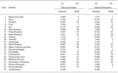
Notes. 1. Intensities are expressed as emissions per unit output. Emissions are measured in kilotonnes of CO2 equivalent. The

unit of output is the amount that can be bought for $1millon in 2004-05.

Adjusted intensities are obtained by attributing the emissions associated with the production of intermediate inputs to the using industry.

Table 2 shows the emissions intensities (i.e., the emissions per unit output) in 2004-05. Emissions are measured in kilotonnes of CO2 equivalent. The unit of output is the amount that can be

(14)

6

Footwear, some produced by 2 Dairy are attributed 15 Other Food Products, and some produced by 33 Gas Supply are attributed to 52 Private Heating. On the other side of the pollution ledger, some of the reduction in emissions resulting from production in the industry 7 Forestry are now attributed to the industries which use forestry products as inputs, particularly 17 Wood Products

and 18 Paper Products. The change to the accounting system reduces the range of the emission intensities by more than half.

The emissions intensities change over time in response to the mitigation policy. The average intensity drops from 0.248 in 2004-05 to 0.208 in 2024-25 in the Basecase scenario, and to 0.148 in the CRPS-5 scenario.

3. The Labour Market Simulations

The labour market effects of the climate change mitigation policy are analysed using the MONASH Labour Market Extension (MLME). This model is designed to be incorporated in the MONASH CGE model (Dixon and Rimmer, 2002), the national model from which the multi-region MMRF model is derived. It describes markets for 81 occupations, the minor groups of the Australian Standard Classification of Occupations. Its purpose is to allow supply constraints on labour by skill to be imposed on demands for labour by industry via the occupational markets. In principle, 67 skill groups are identified, consisting of six education levels cross classified with eleven educational fields plus the residual category No Post-School Qualification. However, three of these categories contained no entries in the base period data and, for operational purposes, the number of groups was reduced to 64. All skill categories are derived from the Australian Standard Classification of Education.

On the supply side, labour by skill can be converted into labour by occupation according to

Constant Elasticity Transformation (CET) functions. Figure 1 presents the idea diagrammatically.

(15)

7

Figure 1 : Skill Transformations between Occupations

Figure 2: Substitution between Occupations in Industries Employment

Occupation 1

Slope = -w2/w1

E2

E1

L21 L22

Employment Occupation 2 L11

L12

Employment Occupation 1

Slope = -w2/w1

E2

E1

L21 L22

Employment Occupation 2 L11

(16)

8

skills can be transformed into any of the 81 occupations. However, if none of a particular skill is used in a particular occupation in the base period, none of it will be used in that occupation in any of the simulations.

Labour of different occupations can be converted, in turn, into effective units of industry specific labour according to Constant Elasticity Substitution (CES) functions. In Figure 2, the position of the isoquant is determined by the demand for labour in the industry. If the wage rate of occupation 2 decreases relative to that of occupation 1, the isocost line becomes flatter, and the producers in the industry can reduce their costs by substituting some of occupation 2 for occupation 1. Hence they change the occupational mix from E1 to E2. In principle, each of the 52 industries can employ any of 81 occupations but, as before, none of a particular occupation will be used by an industry in a simulation if none of it was used by that industry in the base period.

As the isoquant is convex to the origin, the number of hours of occupation 2 required to replace an hour of occupation 1 and remain on the isoquant (i.e., and deliver the same amount of industry-specific labour) increases as the amount of occupation 2 already being used increases. More generally, the efficiency of an additional hour of an occupation in an industry decreases as the number of hours of the occupation already being used in that industry increases. In the MONASH and MMRF model, employment by industry is measured in efficiency units. In the MLME model, separate accounting systems are maintained for labour measured in efficiency units and labour measured in hours. However, results are only reported in terms of the latter.

In MMRF, the average real-wage is initially assumed to be sticky so employment can deviate from its Basecase value in response to the CPRS. Over time, though, it is assumed that real wage adjustment steadily eliminates most, if not all, of the short-run consequences for aggregate employment. This means that, in the long run, the costs of reducing emissions are realised almost entirely as a fall in the average real wage rate, rather than as a fall in aggregate employment. This labour market assumption reflect the idea that in the long-run aggregate employment is determined by demographic factors, which are largely unaffected by the adoption of an emissions reduction policy. Relative wage rates across industries are assumed to remain constant at the levels that prevailed in the base period, 2004-05.

(17)

9

employment by industry and the average wage rate determined by MMRF. That being the case, there is no room for imposing labour supply constraints in MLME and the supply of labour by skill plays no role in the determination of the distributional results. Each industry simply retains the same mix of occupations that it employed in the base period.

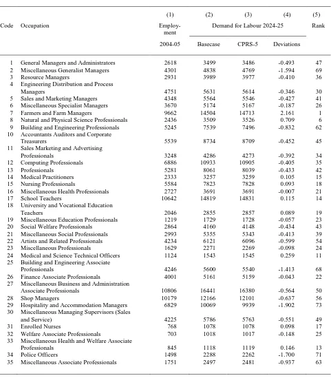
Table 3 presents MLME results for the two simulations. According to the table, employment of the occupation 1 General Managers and Administrators was 2618 thousand hours per week (thpw) in 2004-05. For the Basecase, employment of the occupation is projected to increase to 3499 thpw in the terminal period (i.e., 2024-25). For the CPRS-5 simulation, the increase is only 3486 thpw. Hence, relative to base period employment, the implementation of the mitigation policy results in a reduction in employment of 0.493 per cent. If the 81 ASCO minor groups are reordered according to the increase in employment projected for the terminal period, 1 General Managers and Administrators is ranked 47th.

The occupation with the largest increase is 7 Farmers and Farm Managers, its employment increasing by 2.161 per cent. The source of the increase can be understood in terms of the contributions of the industries which provide employment to the occupation. Table 4 shows the most important contributors, both positive and negative. Not surprisingly, all are agricultural industries. Australia is a large exporter of agricultural and mining commodities, and of processed food. From Table 2, several of these industries (including 1 Sheep and Cattle, 8 Coal and 14 Meat Products) also have high emission intensities. When the CPRS is introduced, their costs increase and their exports fall, inducing a depreciation of the Australian dollar. All export-oriented and import-competing industries benefit from the change in the exchange rate. For industries 4 Grain,

5 Other Agriculture, 2 Dairy and 3 Other Animal Farming, the exchange-rate effect is sufficient to deliver an increase in employment in the terminal period, and hence to deliver an increase in employment of Farmers and Farm Managers. For industry 1 Sheep and Cattle, the emissions-intensity effect outweighs the exchange-rate effect and its employment decreases. However, the resulting negative contribution to Farmers and Farm Managers is more than offset by the contributions of the expanding agricultural industries.

(18)

10

Table 3. Deviations in Demand for Labour, Relative Wage Rates Constant

(1) (2) (3) (4) (5)

Code Occupation Employ- Demand for Labour 2024-25 Rank

ment

2004-05 Basecase CPRS-5 Deviations

1 General Managers and Administrators 2618 3499 3486 -0.493 47

2 Miscellaneous Generalist Managers 4301 4838 4769 -1.594 69

3 Resource Managers 2931 3989 3977 -0.410 36

4 Engineering Distribution and Process

Managers 4751 5631 5614 -0.346 30

5 Sales and Marketing Managers 4348 5564 5546 -0.427 41

6 Miscellaneous Specialist Managers 3670 5174 5167 -0.187 26

7 Farmers and Farm Managers 9662 14504 14713 2.161 1

8 Natural and Physical Science Professionals 2436 3509 3526 0.709 6

9 Building and Engineering Professionals 5245 7539 7496 -0.832 62

10 Accountants Auditors and Corporate

Treasurers 5539 8734 8709 -0.452 45

11 Sales Marketing and Advertising

Professionals 3248 4286 4273 -0.392 34

12 Computing Professionals 6886 10933 10905 -0.405 35

13 Professionals 5281 8061 8039 -0.433 42

14 Medical Practitioners 2333 3257 3259 0.105 15

15 Nursing Professionals 5584 7823 7828 0.093 18

16 Miscellaneous Health Professionals 2727 3691 3691 -0.007 21

17 School Teachers 10642 14819 14831 0.115 14

18 University and Vocational Education

Teachers 2046 2855 2857 0.089 19

19 Miscellaneous Education Professionals 1219 1729 1728 -0.057 23

20 Social Welfare Professionals 2864 4160 4148 -0.434 43

21 Miscellaneous Social Professionals 2993 5355 5343 -0.413 39

22 Artists and Related Professionals 4234 6121 6096 -0.599 54

23 Miscellaneous Professionals 1629 2271 2269 -0.098 24

24 Medical and Science Technical Officers 1124 1543 1545 0.259 11

25 Building and Engineering Associate

Professionals 4246 5600 5540 -1.413 68

26 Finance Associate Professionals 4001 5161 5159 -0.043 22

27 Miscellaneous Business and Administration

Associate Professionals 10806 16441 16380 -0.564 50

28 Shop Managers 10179 12166 12101 -0.637 56

29 Hospitality and Accommodation Managers 6829 10069 9939 -1.902 73

30 Miscellaneous Managing Supervisors (Sales

and Service) 4225 5786 5763 -0.551 49

31 Enrolled Nurses 768 1078 1078 0.098 17

32 Welfare Associate Professionals 703 1018 1017 -0.148 25

33 Miscellaneous Health and Welfare Associate

Professionals 845 1118 1119 0.146 13

34 Police Officers 1498 2288 2262 -1.700 71

35 Miscellaneous Associate Professionals 1751 2497 2481 -0.937 63

(19)

11

Table 3. (continued)

(1) (2) (3) (4) (5)

ment

36 Mechanical Engineering Tradespersons 5157 5530 5500 -0.596 51

37 Fabrication Engineering Tradespersons 3306 3112 3058 -1.639 70

38 Automotive Tradespersons 5736 6617 6587 -0.522 48

39 Electrical and Electronics Tradespersons 7527 8440 8288 -2.021 74

40 Structural Construction Tradespersons 7695 8781 8573 -2.713 77

41 Final Finishes Construction Tradespersons 2387 2866 2801 -2.740 78

42 Plumbers 2547 2949 2874 -2.960 80

43 Food Tradespersons 3007 3769 3748 -0.682 59

44 Skilled Agricultural Workers 709 1032 1035 0.418 10

45 Horticultural Tradespersons 2366 3258 3230 -1.184 66

46 Printing Tradespersons 1078 1116 1123 0.672 7

47 Wood Tradespersons 1485 1337 1362 1.690 3

48 Hairdressers 1476 2245 2220 -1.707 72

49 Textile Clothing and Related Tradespersons 588 528 533 0.775 5

50 Miscellaneous Tradespersons and Related

Workers 2838 3373 3338 -1.240 67

51 Secretaries and Personal Assistants 5218 7533 7500 -0.639 57

52 Advanced Numerical Clerks 3430 4618 4598 -0.599 53

53 Service Workers 1781 2650 2644 -0.325 28

54 General Clerks 4517 6119 6100 -0.413 38

55 Keyboard Operators 2577 3601 3592 -0.342 29

56 Receptionists 4291 6178 6160 -0.425 40

57 Intermediate Numerical Clerks 7537 9778 9752 -0.350 31

58 Material Recording and Despatching Clerks 4134 4978 4961 -0.412 37

59 Miscellaneous Intermediate Clerical Workers 4952 6575 6561 -0.276 27

60 Intermediate Sales and Related Workers 5348 6311 6286 -0.457 46

61 Carers and Aides 7355 10327 10330 0.034 20

62 Hospitality Workers 3737 5602 5522 -2.152 75

63 Miscellaneous Intermediate Service Workers 3970 6057 6026 -0.788 61

64 Mobile Plant Operators 4831 5805 5784 -0.440 44

65 Intermediate Stationary Plant Operators 2498 2520 2448 -2.877 79

66 Intermediate Textile Clothing and Related

Machine Operators 964 855 863 0.860 4

67 Miscellaneous Intermediate Machine

Operators 1703 1656 1665 0.491 8

68 Road and Rail Transport Drivers 12062 12364 12319 -0.369 33

69 Intermediate Mining and Construction

Workers 1899 2006 1948 -3.051 81

70 Miscellaneous Intermediate Production and

Transport Workers 5686 6586 6592 0.098 16

71 Elementary Clerks 1866 2115 2109 -0.352 32

72 Sales Assistants 13189 15676 15586 -0.680 58

73 Miscellaneous Elementary Sales Workers 4273 5428 5402 -0.618 55

74 Elementary Service Workers 3212 5256 5234 -0.688 60

(20)

12

Table 3. (continued)

(1) (2) (3) (4) (5)

ment

75 Cleaners 4965 8147 8118 -0.599 52

76 Process Workers 4849 4669 4680 0.238 12

77 Product Packagers 2236 2463 2473 0.427 9

78 Mining Construction and Related Labourers 4422 5208 5105 -2.342 76

79 Agricultural and Horticultural Labourers 4112 5764 5838 1.808 2

80 Elementary Food Preparation and Related

Workers 2462 3310 3286 -0.973 64

81 Miscellaneous Labourers and Related

Workers 2493 3248 3220 -1.125 65

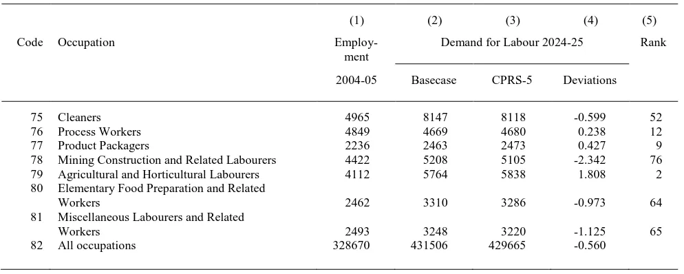
82 All occupations 328670 431506 429665 -0.560

Notes. Columns 1 to 3 are measured in thousands of hours per week.

Column 4 measures the deviations between the demand for labour in the CPRS-5 (column 3) and the Basecase (column 2) simulations expressed as a percentage of base period employment (column 1).

The ranks in column 5 are based on the deviations in column 4.

influenced by the exchange rate depreciation, the former via the export-oriented agricultural industries previously discussed and the latter via the import-competing industry 16 Textiles Clothing and Footwear. The occupation 47 Wood Tradespersons, on the other hand, owes its employment increase to the industry 7 Forestry; it alone has a negative direct emission intensity and a large negative intensity at that. Hence the introduction of the CPRS actually reduces the costs of production in Forestry and its down-stream processing industries 17 Wood Products and

18 Paper Products. The resulting employment increase in Wood Products is largely responsible for the favourable result for Wood Tradespersons.

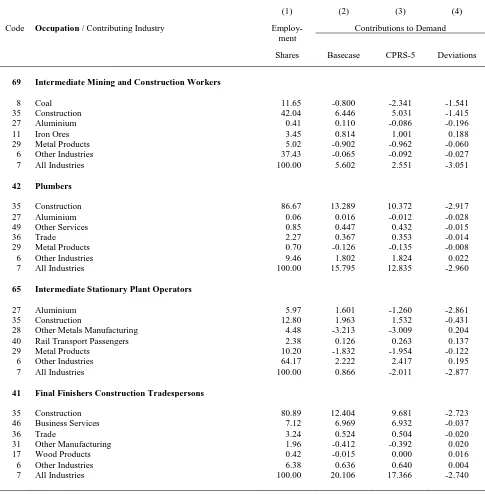
Table 5 is similar to Table 4, but this time it identifies the industry contributors to the occupations which experience the largest reductions in employment in the terminal period. Prominent among them are the high emission-intensity industries 8 Coal and 27 Aluminium. However, the industry

(21)

13

Table 4. Contributions to Deviations in Employment, Expanding Occupations

(1) (2) (3) (4)

Code Occupation / Contributing Industry Employ- Contributions to Employment ment

Shares Basecase CPRS-5 Deviations

7 Farmers and Farm Managers

4 Grains 29.49 19.771 21.711 1.940

1 Sheep and Cattle 34.74 19.104 17.968 -1.136

5 Other Agriculture 18.71 8.420 9.156 0.736

2 Dairy 7.48 2.152 2.585 0.433

3 Other Animal Farming 2.69 -0.674 -0.548 0.126

Other Industries 6.89 1.336 1.398 0.062

All Industries 100.00 50.109 52.270 2.161

79 Agricultural and Horticultural Labourers

5 Other Agriculture 31.89 14.346 15.600 1.254

4 Grains 9.08 6.087 6.684 0.597

1 Sheep and Cattle 10.70 5.881 5.532 -0.350

49 Other Services 13.82 7.295 7.054 -0.241

7 Forestry 0.76 0.010 0.196 0.186

All Industries 100.00 40.168 41.976 1.808

47 Wood Tradespersons

17 Wood Products 35.26 -1.293 0.038 1.331

31 Other Manufacturing 50.50 -10.634 -10.112 0.522

35 Construction 4.49 0.689 0.537 -0.151

36 Trade 5.18 0.839 0.807 -0.032

30 Motor Vehicles and Parts 1.22 -0.340 -0.320 0.020

All Industries 100.00 -9.960 -8.271 1.690

66 Intermediate Textile Clothing and Related Machine Operators

16 Textile Clothing and Footwear 58.67 -13.773 -12.815 0.958

27 Aluminium 0.40 0.108 -0.085 -0.193

15 Other Food Products 2.70 0.028 0.114 0.086

35 Construction 2.04 0.312 0.244 -0.069

Other Industries 26.98 4.027 4.009 -0.018

All Industries 100.00 -11.238 -10.378 0.860

Notes. Column 1 contains employment shares, measured in per cent, for the base period 2004-05.

Columns 2 and 3 contain the industry contributions, measured in percentage points, to the growth in employment of the nominated occupation between 2004-05 and 2024-25.

(22)

14

Table 5. Contributions to Deviations in Employment, Contracting Occupations

(1) (2) (3) (4)

Code Occupation / Contributing Industry Employ- Contributions to Demand

ment

Shares Basecase CPRS-5 Deviations

69 Intermediate Mining and Construction Workers

8 Coal 11.65 -0.800 -2.341 -1.541

35 Construction 42.04 6.446 5.031 -1.415

27 Aluminium 0.41 0.110 -0.086 -0.196

11 Iron Ores 3.45 0.814 1.001 0.188

29 Metal Products 5.02 -0.902 -0.962 -0.060

6 Other Industries 37.43 -0.065 -0.092 -0.027

7 All Industries 100.00 5.602 2.551 -3.051

42 Plumbers

35 Construction 86.67 13.289 10.372 -2.917

27 Aluminium 0.06 0.016 -0.012 -0.028

49 Other Services 0.85 0.447 0.432 -0.015

36 Trade 2.27 0.367 0.353 -0.014

29 Metal Products 0.70 -0.126 -0.135 -0.008

6 Other Industries 9.46 1.802 1.824 0.022

7 All Industries 100.00 15.795 12.835 -2.960

65 Intermediate Stationary Plant Operators

27 Aluminium 5.97 1.601 -1.260 -2.861

35 Construction 12.80 1.963 1.532 -0.431

28 Other Metals Manufacturing 4.48 -3.213 -3.009 0.204

40 Rail Transport Passengers 2.38 0.126 0.263 0.137

29 Metal Products 10.20 -1.832 -1.954 -0.122

7 All Industries 100.00 0.866 -2.011 -2.877

41 Final Finishers Construction Tradespersons

35 Construction 80.89 12.404 9.681 -2.723

46 Business Services 7.12 6.969 6.932 -0.037

36 Trade 3.24 0.524 0.504 -0.020

17 Wood Products 0.42 -0.015 0.000 0.016

7 All Industries 100.00 20.106 17.366 -2.740

Notes. Column 1 contains employment shares, measured in per cent, for the base period 2004-05.

Columns 2 and 3 contain the industry contributions, measured in percentage points, to the growth in employment of the nominated occupation between 2004-05 and 2024-25.

(23)

15

follows that industries which mainly service investment loose out to industries which mainly service the other major components of final demand. Construction is the prime example.

Policy proposals for climate change mitigation are often based on identifying jobs that can be considered to be “green” in some a priori sense. Once identified, the jobs are then recommended for government support of one kind or another as a way of reducing emissions. However, the definitions adopted are often very loose. It may reasonably be thought that a classification based on emission intensities would provide a more rigorous a priori definition, and hence provide a more reliable guide as to the contributions that various jobs might make to the mitigation process. Table 6 provides some evidence on this conjecture where “jobs” are identified with occupations.

(24)

16

Table 6. Emission Intensities and Employment Deviations, Selected Occupations

(1) (2) (3) (4)

Code Occupation Emission Intensities Employment Deviations

Intensity Rank Deviation Rank

7 Farmers and Farm Managers 0.1362 79 2.161 1

8 Natural and Physical Science Professionals 0.0022 8 0.709 6

9 Building and Engineering Professionals 0.0849 76 -0.832 62

14 Medical Practitioners 0.0011 4 0.105 15

15 Nursing Professionals 0.0010 3 0.093 18

17 School Teachers 0.0008 2 0.115 14

18 University and Vocational Education

Teachers 0.0016 5 0.089 19

31 Enrolled Nurses 0.0007 1 0.098 16

39 Electrical and Electronics Tradespersons 0.1436 80 -2.021 74

40 Structural Construction Tradespersons 0.0048 20 -2.713 77

41 Final Finishes Construction Tradespersons 0.0033 15 -2.740 78

42 Plumbers 0.0063 24 -2.960 80

47 Wood Tradespersons 0.0030 13 1.690 3

49 Textile Clothing and Related Tradespersons 0.0044 18 0.775 5

50 Miscellaneous Tradespersons and Related

Workers 0.1104 78 -1.240 67

61 Carers and Aides 0.0016 6 0.034 20

65 Intermediate Stationary Plant Operators 0.0864 77 -2.877 79

66 Intermediate Textile Clothing and Related

Machine Operators 0.0150 42 0.860 4

69 Intermediate Mining and Construction

Workers 0.1538 81 -3.051 81

78 Mining Construction and Related Labourers 0.0202 50 -2.342 76

79 Agricultural and Horticultural Labourers 0.0496 70 1.808 2

82 All occupations 0.0267 82 -0.560 82

Notes. 1. Intensities are expressed as emissions per unit of labour input in 2004-05. Emissions are measured in kilotonnes of CO2 equivalent. Labour is measured in thousands of hours.

2. The deviations in column 3 are the differences between employment in 2024-25 for the Basecase and CPRS-5 scenarios (see Table 4). They are expressed as a percentage of employment in 2004-05.

4. The Income Simulations

The effects of the mitigation policy on the distribution of income are assessed using two related models: the MONASH Income Distribution Extension (MIDE) and the MONASH Microsimulation Extension (MMSE)4. Like MLME, MIDE is designed to be incorporated in the MONASH national CGE model and serves two main functions. Firstly, it contains an aggregate social accounting

4

(25)

17

matrix made up of current and capital accounts for the household sector, corporate trading enterprises, financial trading enterprises and the government sector, and an account for external sector. These accounts identify the amounts of saving, borrowing and lending undertaken by the various institutions, and allow those variables to be constrained if required. Secondly, it describes income sources for 100 household types differentiated by size of income, and expenditure patterns for 600 household types differentiated by size of income (10 groups) and household composition. The two classifications are connected via a (100 x 600) disposable income matrix. This arrangement allows changes in the distribution of income by household to feed back into changes in expenditure by commodity. Again like MLME, MIDE is used in a top-down configuration with MMRF in the present simulations, and hence does not impose any constraints on the results of the latter. The MMSE model consists of a unit record data file containing 13605 person records derived from the Australian Income Distribution Survey (ABS, 1998) but modified to form a fully integrated system with the MLME database and MMRF database when aggregated to the national level. Consistency is imposed by adopting a hierarchy of sources in which the data at each level is a disaggregation of the data at the preceding level. The main components of the hierarchy are:

 the National Accounts organised into an aggregate social accounting matrix,

 the Input-Output Table,

 the Labour Force Survey,

 the Survey of Education and Work;

 the Income Distribution Survey, and

 The Household Expenditure Survey.

(26)

18

matrix is then updated using the RAS method. The updated matrix, in its turn, provides the where-with-all to revise the weights attached to the unit records.

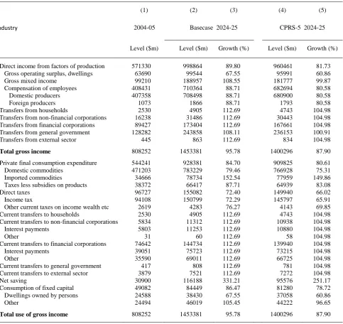
Table 7 shows results for one of the nine institutional accounts that make up the social accounting matrix in MIDE, namely, the Household current account. MIDE contains enough theory to determine the values of all the categories in the account except Net saving, which is the residual between the income and expenditure sides. Note that the theory is not always particularly sophisticated, with several categories assumed to move with GDP.

Table 8 shows the corresponding projections for disposable income. Disposable income (which was $631,510m in 2004-05) in Table 8 can be derived from Total gross income ($808,252m) in Table 7 by subtracting Consumption of fixed capital, Interest payments, Income taxes and Other taxes on income, wealth, etc. As with the output and employment results, the effect of the mitigation policy on incomes is small compared to the income growth that is projected to occur between 2004-05 and 2024-25 whether the policy is adopted or not.

It has already been indicated that a change in Compensation of employees is the cumulative effect of changes in the employment of 81 occupations on the wages of the 13605 persons recognised in the MMSE model. Similarly, a change in Income from own business is the cumulative effect of changes in the return to capital in 17 different industries. The income distribution survey generally contains some persons who sustained losses from self employment in the year of the survey. To accommodate this kind of negative income, an estimate is made of the size of the capital stock in the self–employed sector, and the stock then allocated between the relevant persons in the microsimulation model. In particular, persons who achieved large profits or

(27)

19

Table 7. Household Current Account

(1) (2) (3) (4) (5)

Industry 2004-05 Basecase 2024-25 CPRS-5 2024-25

Level ($m) Level ($m) Growth (%) Level ($m) Growth (%)

Direct income from factors of production 571330 998864 89.80 960461 81.73

Gross operating surplus, dwellings 63690 99544 67.55 95991 60.86

Gross mixed income 99210 188957 108.55 181777 99.87

Compensation of employees 408431 710364 88.71 682694 80.58

Domestic producers 407358 708498 88.71 680900 80.58

Foreign producers 1073 1866 88.71 1793 80.58

Transfers from households 2530 4905 112.69 4743 104.98

Transfers from non-financial corporations 16238 31486 112.69 30443 104.98

Transfers from financial corporations 89427 173404 112.69 167661 104.98

Transfers from general government 128282 243858 108.11 236153 100.91

Transfers from external sector 445 863 112.69 834 104.98

Total gross income 808252 1453381 95.78 1400296 87.90

Private final consumption expenditure 544241 928381 84.70 909825 80.61

Domestic commodities 471203 783229 79.46 766928 75.31

Imported commodities 34666 78734 152.54 77959 149.86

Taxes less subsidies on products 38372 66417 87.71 64939 83.08

Direct taxes 96727 155082 72.40 149940 66.02

Income tax 94108 150799 72.29 145797 65.91

Other current taxes on income wealth etc 2619 4283 76.27 4143 69.85

Current transfers to households 2530 4905 112.69 4743 104.98

Current transfers to non-financial corporations 5834 11312 112.69 10938 104.98

Interest payments 5803 11253 112.69 10880 104.98

Other 31 60 112.69 58 104.98

Current transfers to financial corporations 74642 144734 112.69 139940 104.98

Interest payments 39051 75723 112.69 73215 104.98

Other 35590 69011 112.69 66725 104.98

Current transfers to general government 417 808 112.69 781 104.98

Current transfers to external sector 3879 7521 112.69 7272 104.98

Net saving 30900 116188 331.21 95576 251.17

Consumption of fixed capital 49082 84449 86.47 81280 78.72

Dwellings owned by persons 24588 38430 67.55 37058 60.86

Other 24494 46019 105.45 44222 96.65

(28)

20

Table 8. Household Disposable Income

(1) (2) (3) (4) (5)

Level ($m) Level ($m) Growth (%) Level ($m) Growth (%)

Income from dwellings, landlords

Gross operating surplus 17002 26573 56.29 25624 50.72

less consumption of fixed capital 6563 10258 56.29 9892 50.72

less interest payments 6111 9551 56.29 9210 50.72

Income from own business

Gross mixed income 99210 188957 90.46 181777 83.22

Compensation of employees 408431 710364 73.93 682694 67.15

Actual interest 24786 48062 93.91 46470 87.48

Dividends 12391 24028 93.91 23232 87.48

Unemployment benefits 7621 9891 29.78 9936 30.37

Other taxable benefits 73258 142051 93.91 137346 87.48

Other current transfers, taxable 16779 32535 93.91 31457 87.48

Income from dwellings, owner occupiers

Gross operating surplus 46688 72971 56.29 70367 50.72

Imputed interest 33703 65352 93.91 63187 87.48

Social assistance benefits, non-taxable 20144 39060 93.91 37766 87.48

Other current transfers, non-taxable 48239 93539 93.91 90440 87.48

less Income taxes 94106 150797 60.24 145795 54.93

less Other taxes on income wealth etc 2619 4283 63.56 4143 58.21

Disposable income 631510 1162790 84.13 1119860 77.33

(29)

21

Table 9. Distribution of Household Disposable Income

(1) (2) (3) (4) (5) (6)

Level ($m) Share (%) Level ($m) Share (%) Level ($m) Share (%)

Nominal incomes

Income deciles

1st -429 -0.068 1515 0.130 1384 0.124

2nd 10296 1.630 19058 1.639 18421 1.645

3rd 24052 3.809 44727 3.847 43238 3.861

4th 33975 5.380 63505 5.461 61426 5.485

5th 40127 6.354 74168 6.378 71723 6.405

6th 49311 7.808 90394 7.774 87134 7.781

7th 61876 9.798 112882 9.708 108610 9.699

8th 80639 12.769 146596 12.607 140945 12.586

9th 109810 17.389 199893 17.191 192242 17.167

10th 221854 35.131 410052 35.264 394738 35.249

631510 100.000 1162791 100.000 1119860 100.000

Income percentiles

10th 434 0.069 799 0.069 772 0.069

90th 12783 2.024 23211 1.996 22332 1.994

90th/10th 29.472 29.058 28.938

Real incomes

Income deciles

1st -429 -0.068 1518 0.131 1385 0.124

2nd 10296 1.630 19049 1.647 18324 1.646

3rd 24052 3.809 44705 3.865 43144 3.875

4th 33975 5.380 63326 5.475 61079 5.486

5th 40127 6.354 73902 6.389 71331 6.406

6th 49311 7.808 90021 7.783 86644 7.782

7th 61876 9.798 112272 9.706 107895 9.690

8th 80639 12.769 145833 12.608 140082 12.581

9th 109810 17.389 198809 17.188 191211 17.173

10th 221854 35.131 407247 35.208 392350 35.238

631510 100.000 1156682 100.000 1113444 100.000

Income percentiles

10th 434 0.069 799 0.069 772 0.069

90th 12783 2.024 23087 1.994 22208 1.993

(30)

22 5. Concluding Remarks

The Australian Treasury’s analysis of the economics of climate change mitigation has been called “the most thorough, comprehensive and well documented modelling exercise ever conducted in Australia”5. This paper has sought to build on this modelling effort by extending an associated MMRF analysis to address distributional issues. The Treasury concluded that “large reductions in emissions do not require reductions in economic activity because the economy restructures in response to emission pricing.”6 The results presented here suggest that the same sentiment is apposite for distribution.

This relatively benign assessment is somewhat at odds with much of the policy debate concerning climate change and its mitigation. A suitable example of the kind of response such assessments evoke is provided by the UNEP in its influential 2008 report on green jobs:

“(Some) studies, based on macro-economic calculations, do not focus on green industries but seek to determine the likely overall effect on the economy arising from policies aiming to reduce greenhouse gas emissions or other environmental impacts. They focus on the ways in which production costs may change, how demand for products and technologies may be altered by new regulations and standards, etc. The results of such analyses are heavily influenced by the basic assumptions that go into them. … The nature of these and other assumptions inevitably color the general nature of the findings. Thus, skeptical assumptions about reducing greenhouse gas emissions or other environmental measures will likely produce studies that predict job losses, just as more positive assumptions will yield upbeat results. Most studies agree, however, that the likely impact is a small positive change in total employment.”7

Having drawn attention to the existence of such studies, and to the effect on aggregate activity they predict, the UNEP then proceeds to ignore them throughout the rest of its report. Its attempt to dismiss economy-wide analyses on the grounds that they are “heavily influenced by

5

See Parkinson (2009), p.9. Parkinson is the head of the Australian Department of Climate Change.

6

Australian Treasury (2008), p.137.

7

(31)

23

the assumptions that go into them” is, of course, completely spurious. All analyses are heavily influenced by the assumptions that go into them.

The same kind of idea sometimes surfaces in defence of simple models for analysing distributional issues. It is argued that because the values of behavioural parameters are often not well known, it is desirable to assume no behavioural response and rely entirely on income accounting. But “no behavioural response” is itself an estimate of the values of the relevant behavioural parameters, and is a choice that cannot usually be supported empirically. Similarly, analysts sometimes prefer to estimate the “morning after” effects of a policy change on the grounds that forward-looking analyses are too uncertain. Again, if such analyses were really thought to be of no relevance to the day after “the morning after”, they would be of little interest. Policy analysis cannot escape from adopting positions, either explicitly or implicitly, on all the matters that affect the outcome of the policy under consideration.

More specifically, the results presented here depend in part on the view that Australia is unlikely to experience large increases in unemployment over the forecast period. In that case, persons working in occupations adversely affected by the mitigation policy are deemed to be able to pick up jobs in other occupations. Hence there is little scope for employment changes to impact significantly on income inequality. Similarly, persons on low-incomes may spend a larger share of their budget on electricity, but the variation in budget shares across income groups is not generally large enough to drive substantial changes in inequality and, even then, its effect will be ameliorated by economic adjustment to the change in relative prices.

(32)

24 References

Australian Treasury (2008), Australia's Low Pollution Future: The Economics of Climate Change Mitigation, Canberra, October.

Adams, P.D., J.M Horridge and G, Wittwer (2003), “MMRF-GREEN: A Dynamic Multi-Regional Applied General Equilibrium Model of the Australian Economy”, Working Paper No. G-140, Centre of Policy Studies, Monash University, October.

Centre of Policy Studies (2008), Model Development and Scenario Design: MMRF Modelling to Support a Study of the Economic Impacts of Climate Change Mitigation. Available from

http://www.treasury.gov.au/lowpollutionfuture/consultants_report/downloads/Model_Devel opment_and_Scenario_Design.pdf.

Dixon, P.B. and M.T.Rimmer (2002), Dynamic General Equilibrium Modelling for Forecasting and Policy: A Practical Guide and Documentation of MONASH, North-Holland, Amsterdam. Pang, Felicity. (2014), A General Equilibrium Analysis of Fiscal Incidence in Australia, Ph.D thesis,

Monash University, forthcoming.

Parkinson, M. (2009), “Australia in the Low Carbon Economy”, paper presented to the Australian Financial Review Carbon Reduction Conference, Melbourne, July. Available from

http://www.climatechange.gov.au/en/media/speeches.aspx.