Evaluation of Resilience of randomized RNS
implementation
J´erˆome Courtois1, Lokman Abbas-Turki2, Jean-Claude Bajard1
1
Sorbonne Universit´es, UPMC, CNRS, LIP6, Paris, France
2 Laboratoire de Probabilit´es et Mod´eles Al´eatoires, UMR 7599, UPMC
Abstract. Randomized moduli in Residue Number System (RNS) gen-erate effectively large noise and make quite difficult to attack a secret key Kfrom only few observations of Hamming distancesH = (H0, ..., Hd−1)
that result from the changes on the state variable. Since Hamming dis-tances have gaussian distribution and most of the statistic tests, like NIST’s ones, evaluate discrete and uniform distribution, we choose to use side-channel attacks as a tool in order to evaluate randomisation of Hamming distances . This paper analyses the resilience against Corre-lation Power Analysis (CPA), Differential Power Analysis (DPA) when the cryptographic system is protected against Simple Power Analysis (SPA) by a Montgomery Powering Ladder (MPL). While both analy-sis use only information on the current state, DPA Square crosses the information of all the states. We emphasize that DPA Square performs better than DPA and CPA and we show that the number of observations S needed to perform an attack increases with respect to the number of modulin. For Elliptic Curves Cryptography (ECC) and using a Monte Carlo simulation, we conjecture thatS=O((2n)!/(n!)2).
Keywords: RNS, moduli randomization, Monte Carlo, ECC, side channel at-tack, DPA, CPA, DPA Square
1
Introduction
or CPA [8, 18] or other more recent attacks like second-order DPA [25], template attacks [9] and Mutual Information Analysis (MIA) [6]. For a survey on the different attacks and countermeasures, we refer the reader to [11].
The state transitions depend clearly on the data representation which should be also an assumption made by the attacker. The randomization with respect to an arithmetic system ensures that the computations involved in the execution use different representation for the variables from one execution to another, reducing significantly any prediction on the state transitions for an attacker. We focus in this paper on RNS representation based on the Chinese Remainder Theorem where each value is coded by its residues over a set of co-prime numbers which represents the base of the system.
Beyond the fact that RNS allows natural randomization, the arithmetic is completely independent from the chosen field. Therefore, the methods presented in the paper will be suitable for any cryptosystem such as RSA, ECC, Euclidean Lattice or others. RNS is also adapted to an increase in key sizes induced by the progress of the cryptanalysis and RNS computations can be efficiently par-allelized [2]. For further benefits of RNS, we refer to [13].
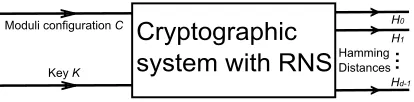
In [4], the authors introduce a Leak Resistant Arithmetic (LRA) using RNS with randomization of moduli. The RNS system is very easy to randomize, es-pecially since there is a great diversity of moduli. Moreover, with Montgomery multiplication algorithm [26], the Montgomery factor strengthen the random behaviour. The goal of randomization according to the involved moduli is to make as unpredictable as possible the secret from the Hamming distance (num-ber of different bits) between two consecutive states that can be detected in the consumption or in any other leak. As sketched on Figure 1, we distinguish two randomness sources given by both the configuration of moduliCand the keyK.
Cryptographic
system with RNS
A
Moduli configuration C
A
Key K
A
H0
H1
Hd-1 Hamming Distances
A
A
...
Fig. 1.Hamming distances with respect to randomness sources
H = (H0, ..., Hd−1) are the Hamming distances computed through the ex-ecution of the Montgomery Power Ladder (MPL) algorithm associated, in our examples of this paper, to ECC. When the implementation is public and is free of bugs, it is clear that the random vectorH = (H0, ..., Hd−1) is completely mea-surable with respect to the couple of random variables (K, C). Consequently, more the noise generated by C is important more the link between K and H
marginal distribution ofH andK. The perfect noise must fulfill
L(H, K) :=L(H|K)L(K) =L(H)L(K). (1)
or equivalently L(H|K) = L(H) meaning that K must not provide any infor-mation onH. Although 1 is impossible to obtain because eachHi as a function of K and C will always depend onK, it tells us that the independence of the coordinates of H= (H0, ..., Hd−1) is not necessary to have a perfect noise.
This paper studies the distinguishability between L(H|K) and L(H|K0) (K 6= K0) with respect to the number of moduli n randomized in the RNS representation, denoted also by RNSn. Nevertheless, because studying L(H|K) for the whole vectorH is computationally barely possible, we develop a strategy based on few Hamming distances∼10 that provide the most valuable informa-tion on the keyK. Unlike DPA and CPA that use only the marginal information associated to each step, our conditional strategy combined with DPA Square use a cross-information based on∼10 Hamming distances. This DPA Square notion extends naturally the DPA when we assume thatH = (H0, ..., Hd−1) has a mul-tivariate Normal distribution. DPA Square has the monotonicity benefit since the sizeSof the sample that makes an attack possible increases with respect to
n. Therefore, our main contribution can be summarized in the following points:
1) We show that the cryptographic system has to be resilient with respect to cross-information attack and not only attacks that use marginal information. 2) The randomization makes CPA inefficient and we explain why MIA applied
to the randomization fails.
3) The DPA results are inconsistent with the level of randomization and we show that second-order DPA does not overcome this inconsistency.
4) We present the DPA Square with an asymptotic error which can be used as a threshold for an attack.
5) Unlike DPA, the sizeSto perform an attack with DPA Square is monotonous.
The contributions 1) to 5) are general and can be applied for other crypto-graphic protections. We make the strong assumption that the attacker has access to the Hamming distances. The noise created by the random moduli would add to the hardware noise in real applications. Our work studies the impact of moduli randomization on Hamming distances independent from hardware aspects. We use 112 bits ECC curve essentially to illustrate the results and conjecture that
The rest of this paper is arranged as follows. In Section 2, we briefly describe the moduli randomization of the RNS representation in the Montgomery algo-rithm applied for ECC. Section 3 explains the main reasons why a resilience of a system should rather focus on∼10 successive Hamming distances. Section 4 details our attack based on DPA Square and studies the size S of observations needed to achieve it.
There is not material implementation in this study because it is not useful or even counterproductive because we want to know the added noise by the randomization of moduli.
2
MPL using RNS representation applied to ECC
In Section 2.1, we explain briefly the randomization technic based on RNS rep-resentaion for Montgomery multiplication. Then, Section 2.2 clarifies the way the Hamming distances are computed through the successive steps of the MPL.
2.1 Montgomery for RNS modular multiplication
In [26], P. Montgomery introduced an algorithm of modular multiplication to avoid trial division by large numbers. The RNS version of this algorithm is the starting point of the randomization used in [1]. We summarize this method with a presentation that is quite similar to the one in [3].
We denote|a|m =a mod m and J1, nK:= {1, ...n}. When aand m are
co-prime, we set|a|−1
m :=a−1 mod mto be the inverse ofamodulom. Introducing the RNS basisBn ={m1, ..., mn} of pairwise coprime moduli, the Chinese Re-mainder Theorem ensures the existence of a ring isomorphism betweenZM and Zm1× · · · ×Zmn withM =
Qn
i=1mi. Thus, for any positive integer X strictly smaller than M
X =
n
X
i=1
xi|Mi|− 1 miMi
!
modM (2)
withxi:=|X|mi =X modmi andMi =M/mi.
Let Ben = {me1, ...,men} be another RNS basis of pairwise coprime moduli that are also coprime withBn i.e.mi andmfj are coprime for eachi∈J1, nKand j∈J1, nK. For a numberX that is strictly smaller thanMf=
Qn
i=0mei, we use the
notation {xe1, ...,xen} for the decomposition of X on Ben. Using these notations
Algorithm 1RNSnmodular multiplication
Input A residue baseBn={m1, ..., mn}whereM =Qni=0mi
A residue baseBen={me1, ...,men}whereMf= Qn
i=0meiwithgcd(M,Mf) = 1
A modulusN expressed inBnandBenwithgcd(N, M) = 1,gcd(N,Mf) = 1,
0<(n+ 2)2N < M and 0<(n+ 2)2N < f
M An IntegerAexpressed inBnandBen
An IntegerBexpressed inBn andBenwithAB < N M
Output An integerRexpressed inBnandBensuch thatRmodN=ABM−1modN
Procedure
Q←((−(A×RN SB))RN S)/RN SN in baseBn
Extension 1 OfQfromBn toBen
R←(A×RN SB+RN SQ×RN SN)/RN SM in baseBen
Extension 2 ofR fromBen toBn
end Procedure
Since many modular multiplications are needed in ECC or RSA, one should consider the Montgomery form ofAandB as inputs to Algorithm 1. This trick allows to circumvent dealing withABM−1modN as an output. We recall that the Montgomery form ofAis given byAM modN. OnceMMfmodNis known,
this form can be obtained with Algorithm 1 applied to A and MMfmodN
provided that we exchangeBn andBen since
A× |MMf|N ×Mf−1=AMmodN.
To recover the appropriate expression, we need to perform a final pass in Algorithm 1 for 1 and (AM)(BM)M−1modN that yields to
|(AM)(BM)M−1|N × |1|N ×M−1=ABmod N.
We point out that precomputing|MMf|N instead of |M2|N, as proposed in [3], is justified by the randomization procedure explained latter in this section.
For extension 1 in Algorithm 1, we use a raw method to prevent heavy computations due to mixed radix systems [5] . Thus, to extend in base Ben =
{me1, ...,men}, we calculate
e
qj =
n X i=1 qi
Mi−1
m i m i Mi e mj
for eachj∈J1, nK (3)
we obtain Qe=
n X i=1 qi
Mi−1
m i m i
Mi=Q+α×M withα∈J1, nK (4)
To evaluate α, we use Shenoy-Kumaresan method [28, 3] for extension 2 in Al-gorithm 1. In contrast to Kawamura Extension [17], Shenoy-Kumaresan allows a larger choice of moduli it also involves an extra modulomxsince
α= Mf −1 m x ( n X j=1 e xj Mf −1 j e mj f Mj m x
− |X|m
Subsequently,xi=|X|mi can be computed using
xi=
n X j=1 e xj Mf −1 j e mj f Mj e mj
− |αM|
e mj m i . (6)
The Shenoy-Kumaresan extension requires thatN has to fulfill (n+ 2)2N <
M. The latter inequality with AB < N M makes R < (n+ 2)N. To obtain
R <2N at the very end of an ECC, we use mixed radix representation [5].
2.2 Measuring Hamming distances in our implementation
ECC is usually implemented as an asymmetric cryptographic algorithm in par-ticular for the Integrated Encryption and Decryption Scheme [22, 30]. Alice en-crypts a text with the public key of Bob. The cyphertext contains a pointGof the elliptic curve. With his private keyK, Bob calculates [K]Gto decrypt the cyphertext. ECC is more commonly implemented for the Diffie-Hellman protocol to exchange key via the network.
Before each ECC execution, we perform a random pick ofnmoduli{m1, ..., mn} among{µ1, .., µ2n}for baseBn and the remaining moduli set the baseBen. This
random choice is based on a standard drawing without replacement.
To compute [K]G on an elliptic curve and protect against Simple Power Analysis (SPA)[15], we use the binary version of MPL detailed in Algorithm 2. First, we compute both the Montgomery Form A0 of Gand A1 the double of
A0. Then, if the bit valuebi ofK is one, A0 is added to A1 memorized in A0 and A1 is doubled. Otherwise, A1 is added to A0 memorized in A1 and A0 is doubled.
The elliptic curve domain ofE(FN) is defined by: A finite fieldFN with N a prime number, two elements a andb ∈FN, an equation E :y2 ≡x3+ax+
bmodN, G(xG, yG) a point base of E(FN) andnG is a prime number that is the order ofGonE(FN).
In our implementation, we use the elliptic curves recommended by Certicom [30] employing Jacobian coordinates that avoid the division and reduce compu-tations [24, 10, 14]. Each point is defined by three Jacobian coordinates (X;Y;Z) with the affine representation (X/Z2;Y /Z3). Although there is no uniqueness of the Jacobian representation, computing the Hamming distances on (X;Y;Z) produce more information than computing them on (X/Z2;Y /Z3).
Associated to the equationE isY2=X3+aXZ4+bZ6, (X;−Y;Z) is the inverse of (X;Y;Z) and the infinite point is chosen to be equal to (1; 1; 0). The addition and doubling operations can be found in [24].
Algorithm 2Montgomery Powering Ladder for ECC in RNSn
Input A pointG= (X;Y; 1) in Jacobian coordinates written in RNS representation A keyKwith a binary representationK= 2d−1b0+ 2d−2b1+...+ 2bd−2+bd−1
Output
A0= [K]Gin Jacobian coordinates
(Hi)i∈{0,..,d−1}, the Hamming distances Procedure
Choose a random base permutation
A0= (|XM|N,|Y M|N,|M|N),Montgomery form of G
A1= [2]A0
H0=Hamming Weight of (A0, A1)
fori=1 to d-1do A00=A0 etA01=A1
Abi=Abi+Abi Abi= [2]Abi
Hi= Hamming distance between(A0, A1)and (A00, A
0
1)
end for
ResultA0= (|X0M|N,|Y0M|N,|Z0M|N))in Montgomery form
Return to the Non-Montgomery form with mixed radix [5] A0= (|X0|N,|Y0|N,|Z0|N)
end Procedure
3
A conditional attack strategy and limitations of CPA,
DPA, second-order DPA and MIA
Since Hamming distances have gaussian distribution (see figure 3 b) and most of the statistic tests, like NIST’s ones [31], evaluate discrete and uniform dis-tribution, we choose to use side-channel attacks as a tool in order to evaluate randomisation of Hamming distances.
The randomization of moduli generates effectively noisy data. Because of the lack of structure in Hamming distances, it is quite difficult for an attacker to develop a denoising procedure. Consequently, an attack should target the Hamming distances that provide the most exploitable information on the secret key K. When the latter fact is studied in Section 3.1, Section 3.2 shows that CPA is impossible to use and the sizeSof observations to achieve a DPA attack is not monotonous with respect to the number of moduli. Section 3.3 discusses the adaptation of more recent attacks to RNS randomization.
From now on, we denoteS the size of simulations.
3.1 Sufficient information and conditional attack
The following three properties of Hamming distances are presented:
β) For fixed choice of moduli, the correlation between Hamming distances de-creases significantly with respect to the lag that separates each couple.
γ) Under randomization of moduli, each Hamming distance Hi has a normal distribution. This remark shall not make completely absurd the assumption that the whole vectorH is Gaussian.
These are important properties as they allow to put in place an efficient attack based on the first few Hamming distances. Once the first few bits associated to the first Hamming distances are known, we attack only few following bits conditionally on the fact that we found the first and so on till we find the whole secret K.
As for propertyα), at each stepiof MPL detailed in Algorithm 2, we study the dependence between the random variablesK andHi that take respectively their values on integers in [0,2p[ and [min(Hi), max(Hi)] (Maximum/minimum taken on the realizations of these bounded random variables). In order to reduce the complexity of computations and increase the Monte Carlo accuracy, we use appropriate subdivisions (appropriate parametersp0, qandλ) of:
a) [0,2p[= 2p0−1
[
k=0
Ik = 2p0−1
[
k=0
[k2p−p0,(k+ 1)2p−p0[,(p0< p)
and
b) [min(Hi), max(Hi)] = q−1
[
j=0
Hi j with
Hi
0= [min(Hi), min(Hi) +λ[,H i
q−1= [max(Hi)−λ, max(Hi)],
Hij= [min(Hi) +λ+j, min(Hi) +λ+ (j+ 1)[ for
j= 1, . . . q−2 where= max(Hi)−min(Hi)−2λ
q−2
and the choice ofλis closely linked to the mean and the standard deviation ofHi which has a Gaussian distribution. The accuracy of Monte Carlo was quantified thanks to the 95% confidence interval; with 95% chance we have at most a 10% relative error.
As introduced informally in (1), the dependence is quantified through the dis-tance between the probability of the productP Hi∈ Hij, K ∈Ik
=P(K∈Ik)
P Hi∈ Hji|K∈Ik
and the the product of probabilitiesP Hi∈ Hij
P(K∈Ik). For the subdivisions a) and b), we compute this distance using the Total Varia-tion to Independence (TVI) [20] given by
TVIi=
1 2
2p0−1 X
k=0
q−1 X
j=0
P(K∈Ik)
P
Hi∈ Hij
−PHi∈ Hij|K∈Ik
The value ofP(K∈Ik) is known since we draw uniformly an integer value on [0,2p[. However, the valueP H
i∈ Hij|K∈Ik
, and subsequentlyP Hi∈ Hij
, is approximated using Monte Carlo simulation. For more mathematical details on Monte Carlo simulation we refer the reader to [16].
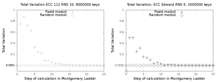
In Figure 2, we calculate TVIifor each step in MPL either for a fixed choice of moduli or when they are randomized. Consequently, when the moduli configura-tion is fixed we draw only independent keys{Kl}
1≤l≤S and when the moduli are randomized we draw independent couples {(Kl, Cl)}1≤l≤S of keys and moduli configurations. The Monte Carlo approximation is then given either by
P Hi∈ Hij, K∈Ik
≈ 1
S
S
X
l=1 1{H
i(Kl)∈Hij
TKl∈I
k}.
or by
P Hi∈ Hij, K ∈Ik≈ 1
S
S
X
l=1 1{H
i(Kl,Cl)∈Hij
TKl∈I
k}.
We simulate withS= 8×10⁶orS= 106in order to have a sufficiently accurate results to compute TVI. We use the random number generator proposed in [19] that is appropriate computationally and statistically for Monte Carlo simulation.
Fig. 2.Total variation as a function of the calculation step.
Regarding property β), we approximate the covariance of each couple of Hamming distances with a Monte Carlo simulation on keys for a fixed choice of moduli
Cov(Hi, Hj)≈
1 S
S
X
l=1
Hi(Kl)Hj(Kl)−
1 S
S
X
l=1
Hi(Kl)
1 S
S
X
k=1
Hj(Kk).
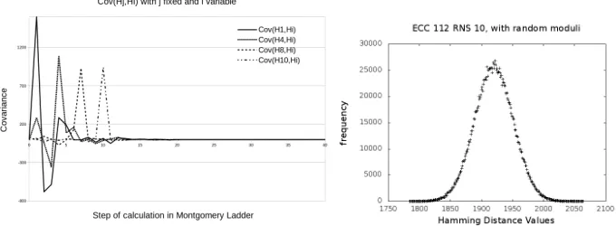
We get the results presented in Figure 3 (a) for the covariance H1, H4, H8 and H10 with the other Hamming distances. In Figure 3 (a), the fact that
|Cov(Hi, Hi±l)|l≥0 decreases with respect to the lag l is due to the gap in bits that separatesHi andHi±l.
It is propertyγ) that makes the covariance very important. Indeed, in a mul-tivariate Gaussian vector, each two coordinates are independent if and only if their covariance is equal to zero. When it is not obvious to show numerically the multivariate Normal distribution, a chi Square test does not disapprove the Gaussian distribution of each Hamming distance Hi when moduli are random-ized. We also present in Figure 3 (b) a histogram associated toH10that shows a bell-shaped distribution. For more mathematical details on multivariate Normal distribution, we refer the reader to [16].
Fig. 3. (a) RNS10,Cov(Hj, Hi)j=1,4,8,10. (b) Frequency ofH10, 2e6 computations.
3.2 Unreliable CPA and inconsistent DPA
The essential result of Section 3.1 is that an effective attack should be based on the first ∼10 computation steps. Once the bits associated to some of these steps are known, one should fix them to continue an attack with the following
dependence on the secret key K and we waste information if we use only the marginal distributions.
Unfortunately, CPA and DPA attacks are not conceived to take advantage of this cross-information. Although CPA and DPA are attacks on power con-sumption, we apply them directly on Hamming distances. We focus rather on the pure software information without hardware noise which can be justified by leakage models presented in [21] between the power consumption and the Hamming distances.
A CPA attack on Hamming distances is based on the correlation that exists at step i between observations Hi(K, Cl) on the real key K and simulations
Hi(K0, Cl+S) on the guessed oneK0 which yields
ξi=
1 S
S
X
l=1 h
Hi(K, Cl)−Hi(K, C)
i h
Hi(K
0
, Cl+S)−Hi(K
0 , C)i
v u u t
1 S
S
X
l1=1 h
Hi(K, Cl1)−Hi(K, C)
i2 1
S
S
X
l2=1 h
Hi(K0, Cl2+S)−Hi(K0, C)
i2
(8)
where
Hi(K, C) =
1 S
S
X
j=1
Hi(K, Cj) and Hi(K0, C) =
1 S
S
X
k=1
Hi(K0, Ck+S). (9)
The lag +S is not usual in the expression (8) of ξi, but it is natural since the moduli configurations{Cl}
1≤l≤S used by the system attacked is supposed to be independent from the moduli configuration{Cl}
S+1≤l≤2S used by the attacker. The independence of the sequence{Cl}
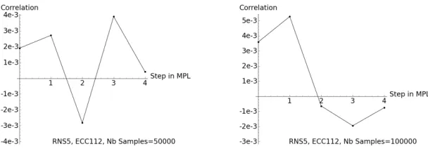
1≤l≤2S makes the use of CPA completely irrelevant as shown in Figure 4. We use 0xdeeefbf7 as the key under attack and 0xffffffff is used as a distinguisher.
Fig. 4.RNS5, Correlation between 0×f f f f f f f fand 0×deeef bf7, 50000 and 100000 samples. Nothing appears at bit 2 and the correlations are too small.
DPAi =Hi(K, C)−Hi(K0, C), (10)
where Hi(K, C) andHi(K0, C) are defined in (9). Unlike for CPA attack, the lag +S involved in the expression of DPAi is less disturbing because, by the law of large numbers, 1
S
PS
k=1Hi(K0, Ck+S) and S1P S
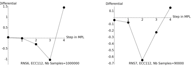
k=1Hi(K0, Ck) converge to the same value asS → ∞. As a consequence, although not perfect, the DPA can be used for an attack whenS is big enough. The fact that we do not know how big S must be (except doing very coarse domination) makes DPA difficult to use. Indeed, as shown in Figure 5, sometimes we even need a biggerS for an RNS with less randomized moduli!
Fig. 5. RNS6 and RNS7: DPA between 0×f f f f f f f f and 0×deeef bf7 with re-spectively 1000000 and 90000 samples. A jump appears for the bit 2 for RNS7 as we expected but the jump is not obvious for RNS6 and we needed more samples to have this little jump
3.3 Further attacks: Second order DPA, MIA and template attack
Like in Section 3.2, we focus only on the pure software information given by Hamming distances. Generally DPA, MIA and template attack are used when the leakage information is observed with a hardware noise. In our pure software study, the noise is due to the RNS randomization that reduces the dependence between the secretK and Hamming distances.
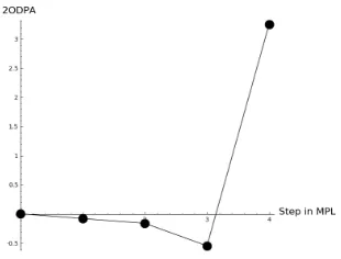
We make a simulation of second order DPA (2ODPA) as follow:
2ODP A0=DP A0 (11)
Fig. 6.RNS6: Second order DPA between 0×f f f f f f f fand 0×deeef bf7 with 1000000 samples.
According to Figure 6, we see that the second order DPA on Hamming dis-tances does not improve the results of DPA presented in Figure 5 (left part). This can be explained by the absence of a heterogeneity in the code between two steps of computations and thus between two successive Hamming distances. Moreover, the second order DPA defined in [25] (Proposition 2) involves marginal information since it averages on the realizations of one random variable defined as the difference between the power consumptions of two successive steps.
Applying template attack [9] on Hamming distances should provide better results than DPA. Indeed, template attack is based on a maximum likelihood approach with a learning phase. The performance of this method is however limited by equation (2) of [9] related, in our context, toPp
i=0|DPAi|with DPAi expressed in (10). As a future work, we would like to compare DPA Square with template attack on RNS randomized systems.
Regarding MIA [6] applied to Hamming distances, we saw clearly in Fig-ure 2 that the TVI is almost equal to zero when we perform randomization. Consequently, it is computationally very complex to develop an attack based on the mutual information for RNS randomized systems. MIA implementation involves the approximation of the logarithm of a probability which is much more computationally involving than the probability itself.
4
A conditional attack strategy with DPA Square,
Thanks to the marginal Gaussian behaviour of Hamming distances announced in property γ) of Section 3.1, it is not absurd to assume that the vector H
of Hamming distances has a multivariate Normal distribution. With the latter assumption, H is completely specified by its mean vector and its covariance matrix. Section 4.1 presents the mathematical tools for DPA Square and Section 4.2 provides. the numerical results.
Con-sequently, from now on, H0 and Hd−1 designate respectively the first and the last Hamming distance involved in each part of the attack.
4.1 Theoretical basis of DPA Square
When the DPA is an attack on the mean vector of H, the DPA Square is an attack on its covariance matrix. The DPA Square has then a big advantage on the DPA because it uses the cross-information given by the different Hamming distances. We have chosen the name DPA Square instead of second-order DPA since the latter was already used for another DPA concept in [25]. The second-order DPA uses differences of differences of Hamming distances whereas the DPA square uses the difference of elements of the covariance matrix.
Unlike the DPA, which is unpredictable (see figure 5), the number of samples to succeed the DPA square is increasing with respect to the number of moduli as we can see on figure 9. Among the original contributions of this paper is the asymptotic quantification of the number of observations needed for an attack. This contribution was possible thanks to DPA square in contrast to DPA which is much less conclusive.
AssumeH = (H0, ..., Hd−1) Gaussian, its mean value isE(H) and letσ2(Hi) be the variance of each coordinate. For a fixed key K, studying the covari-ance matrix of H(K) is equivalent to study the covariance matrix of Y(K) = (Y0(K), ..., Yd−1(K)) with Yi(K) = Hi(Kσ()H−E(Hi(K))
i(K)) which will be denoted by
ΓK =
E(tY(K)Y(K)) which provides
ΓK =
var(Y0(K)) cov(Y0(K), Y1(K)) . . . cov(Y0(K), Yd−1(K))
cov(Y1(K), Y0(K)) var(Y1(K)) . . . cov(Y1(K), Yd−1(K)) ..
. ... . .. ...
cov(Yd−1(K), Y0(K))cov(Yd−1(K), Y1(K)). . . var(Yd−1(K))
Using a sample of sizeS, ΓK is approximated byΓeK and we computeΓeK
0
associated to a guessed keyK0
e
ΓK = 1
S
S
X
j=1
tY(K, Cj)Y(K, Cj),
e
ΓK0 = 1
S
S
X
j=1
tY(K0, Cj+S)Y(K0, Cj+S)
then compute the distance using Frobenius normk · k.
Thanks to the Central Limit Theorem, we can assume thatΓeK =ΓK+δK
andΓeK
0
=ΓK0 +δK0 where√SδK and√SδK0 are asymptotically matrices of centred Gaussian variables with a variances smaller or equal to 1. We define then the DPA Square
DPA2 = 2kΓeK−ΓeK
0
Because
kΓeK−ΓeK
0
k2= X
0≤i,j≤d−1
(ki,j−ki,j0 +δi,j−δi,j0 ) 2
≤2 X 0≤i,j≤d−1
(ki,j−ki,j0 ) 2+ (δ
i,j−δ0i,j) 2
and√S(δi,j−δ0i,j) has asymptotically a normal distributionGi,jwith a variance smaller or equal to 2 thus
E
h
kΓeK−ΓeK
0
k2i≤2 X
0≤i,j≤d−1
(ki,j−k0i,j)2+ 2E
X
0≤i,j≤d−1 (
√
2
√
SGi,j)
2
≤2 X 0≤i,j≤d−1
(ki,j−k0i,j) 2
+ 4
S
X
0≤i,j≤d−1 EG2i,j
E
h
kΓeK−ΓeK
0
k2i≤2 X
0≤i,j≤d−1
(ki,j−ki,j0 ) 2+4d2
S = 2kΓ
K−ΓK0k2+4d2
S .
(14)
This latter expression tells that one has to useS big enough to do an attack and decrease the asymptotic error term 4d2
S when compared to 2kΓ
K−ΓK0k2.
4.2 Numerical results of DPA Square
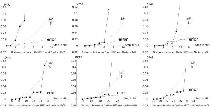
In order to have an efficient attack based on DPA Square, 2kΓK−ΓK0k2 has to be bigger than 4Sd2. Because we do not know the value of 2kΓK−ΓK0k2, we replace it in our attacks by DPA2 = 2kΓeK−ΓeK
0
k2.
Fig. 7.DPA2 in RNS5 on ECC112 withS= 4000: Each new jump over 4Sd2 gives the index of the bit that is equal to zero.
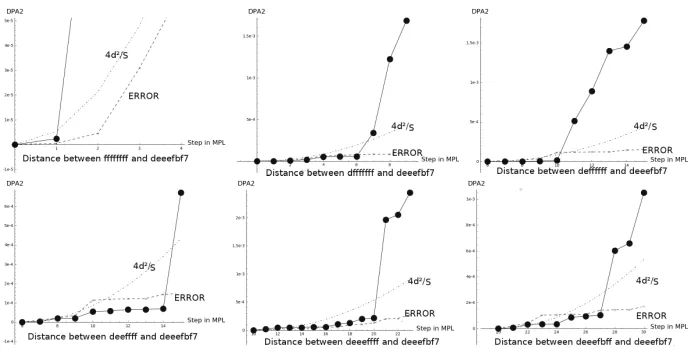
Regarding RNS10, we needed S ≥2500000 to do our attack illustrated for two bits in Figure 8.
Fig. 8.DPA2 in RNS10 on ECC112 withS = 2500000: Each new jump over4Sd2 gives the index of the bit that is equal to zero.
Fig. 9.Attack with DPA2: Size of observationsSto attack the first 10 bits of 0xdeeefbf7 with respects to the number of moduli
Finally we show some results of DPA Square implementation on Edward curve 25519 in Figure 10.
Fig. 10. DPA2 in RNS9 on ECC Edward 25519 of 255 bits withS = 750000: Each new jump over 4d2
5
Conclusion and future work
In this work, we presented the notion of DPA Square that takes advantage of the cross-information in the Hamming distances. This provides an efficient attack even for cryptographic systems protected by RNS randomization. We showed however that this efficiency decreases as the number of needed observations is of the order of (2n)!/(n!)2.
We have started testing further the RNS randomization, especially we would like to provide t-test [12, 29] results in a future work. We are also projecting to implement template attack [9] on RNS randomization and compare it with DPA Square.
References
1. J.A. Ambrose, H. Pettenghi and L. Sousa, “DARNS:A randomized multi-modulo RNS architecture for double-and-add in ECC to prevent power analysis side channel attacks”, Asia and South Pacific Design Automation Conference, pp. 620–625, 2013. 2. S. Antao, J.C. Bajard and L. Sousa, “RNS-Based Elliptic Curve Point Multiplication for Massive Parallel Architectures”, The Comput. J. Oxford J., vol. 55(5), pp. 629– 647, 2011.
3. J.C. Bajard, L.S. Didier and P. Kornerup, “Modular Multiplication and Base Ex-tensions in Residue Number Systems”, IEEE symposium on computer arithmetic, pp. 59–65, 2001.
4. J.C. Bajard, L. Imbert, P.Y. Liardet, Y. Teglia, “Leak Resistant Arithmetic”, Cryp-tographic Hardware and Embedded Systems, Springer LNCS vol. 3156, pp. 62–75, 2004.
5. J.C. Bajard and T. Plantard, RNS bases and conversions. LIRMM UMR 5506, University of Montpellier 2, France.
6. L. Batina, B. Gierlichs, E. Prouff, M. Rivain, F.X. Standaert and N. Veyrat-Charvillon, “Mutual Information Analysis: a Comprehensive Study”, J. Cryptol. 24, pp. 269–291, 2011.
7. D.J. Bernstein, T. Lange, ”Faster addition and doubling on elliptic curves” in: Asiacrypt 2007 vol. 19, pp. 29–50, 2007.
8. E. Brier, C. Clavier and F. Olivier, “Correlation Power Analysis with a Leakage Model”, Cryptographic Hardware and Embedded Systems, Springer LNCS vol. 3156, pp. 16–29, 2004.
9. S. Chari, J. R. Rao and P. Rohatgi, “Template Attacks”, Cryptographic Hardware and Embedded Systems, Springer LNCS vol. 2523, pp. 13–28, 2003.
10. H. Cohen and G. Frey,Handbook of Elliptic and Hyperelliptic Cryptography. Chap-man & Hall, 2006.
11. J. Fan, I. Verbauwhede, “An Updated Survey on Secure ECC Implementations: Attacks, Countermeasures and Cost”, in: Naccache, D. (ed.) Quisquater Festschrift, Springer LNCS vol. 6805, pp. 265–282, 2012.
12. G. Goodwill, B. Jun, J. Jaffe and P. Rohatgi, A testing methodology
for side channel resistance validation. In NIST non-invasive attack
test-ing workshop, 2011. http://csrc.nist.gov/news events/non-invasive-attack-testtest-ing- events/non-invasive-attack-testing-workshop/papers/08 Goodwill.pdf .
13. N. Guillermin,Impl´ementation mat´erielle de coprocesseurs haute performance pour
14. D. Hankerson, A. Menezes and S. Vanstone,Guide to Elliptic Curve Cryptography. Springer, 2004
15. T. Izu and T. Takagi, “A fast parallel elliptic curve multiplication resisitant against side channel attacls”, International Workshop on Public Key Cryptogra-phy, Springer LNCS vol. 2274, pp. 280–296, 2002.
16. J. Jacod and P. Protter, Probability Essentials, second edition, Springer-Verlag, 2003.
17. H. Kawamura, M. Koike, F. Sano, and A. Shimbo, “Cox-Rower Architecture for Fast Parallel Montgomery Multiplications”, EUROCRYPT, pp. 523–538, 2000. 18. P. Kocher, J. Jaffe, B. Jun and P. Rohatgi, “Introduction to differential power
analysis”, J. Cryptogr Eng, 1, pp. 5–27, 2011.
19. P. L’Ecuyer, R. Simard, E. J. Chen, and W. D. Kelton, “An Objected-Oriented Random-Number Package with Many Long Streams and Substreams”, Operations Research, vol. 50(6), pp. 1073–1075, 2002.
20. D.A.Levin, Y. Peres and E. L. Wilmer, “Markov Chains and Mixing Times”, Amer-ican Mathematical Soc. ISBN 9780821886274
21. S. Mangard, E. Oswald and T. Popp,Power Analysis Attacks, Springer, 2007. 22. G. Mart´ınez, H. Encinas, S. ´Avila: A Survey of the Elliptic Curve Integrated
En-cryption Scheme, JCSE, 2, 2 (2010), 7-13.
23. M. Medwed and C. Herbst, “Randomizing the Montgomery Multiplication to Repel Template Attacks on Multiplicative Masking”, in COSADE, 2010.
24. N. Meloni, “New Point Addition Formulae for ECC Applications”, International Workshop on the Arithmetic of Finite Fields, vol. 4547, pp. 189–201, 2007. 25. T.S. Messerges, “Using second-order power analysis to attack DPA resistant
soft-ware”, Cryptographic Hardware and Embedded Systems, Springer LNCS vol. 1965, pp. 238–251, 2000.
26. P. Montgomery, “Modular multiplication without trial division”, Mathematics of Computation , vol. 44(170), pp. 519–521, 1985.
27. G. Perin, L. Imbert, L. Torres and P. Maurine, “Attacking Randomized Exponen-tiations Using Unsupervised Learning”, COSADE, Springer LNCS vol. 4547, pp. 144–160, 2014.
28. A.P . Shenoy and R. Kumaresan, “Fast base extension using a redundant modulus in RNS”, IEEE Transactions on Computer, vol. 38(2), pp. 292–296, 1989.
29. T. Schneider and A. Moradi, “Leakage assessment methodology”, J. Cryptographic Engineering, vol. 6(2), pp. 85–99, 2016.
30. September 20, 2000 Version 1.0 and 2.0: STANDARDS FOR EFFICIENT CRYP-TOGRAPHY Recommended Elliptic Curve Domain Parameters, Certicom Re-search.