Stellar evolution and the Standard Solar Model
ScillaDegl’Innocenti1,2,∗
1Physics Department, Pisa University, Largo B. Pontecorvo n.3, I-56127 Pisa 2INFN, Sezione di Pisa, Largo B. Pontecorvo n.3, I-56127 Pisa
Abstract.This contribution is meant as a very brief introduction to the princi-pal concepts of stellar physics. First the main physical processes active in stellar structures will be shortly described, then the most important features during the stellar life-cycle up to the central H exhaustion will be summarized with partic-ular attention to the description of solar models.
1 Stellar observables
Information about astronomical objects mainly arise from the emitted electromagnetic waves at all possible wavelengths. The most important observable is the luminosity, that is the total energy emitted per unit time. For stars the other fundamental global observable is the color, which is the spectral distribution of the emitted energy that can be directly connected with the temperature of the stellar surface (more precisely one should speak about photosphere, the stellar region from which one can directly receive photons). This because, for almost the whole stellar structure (but the external parts of the atmosphere), photon-matter interac-tions are so efficient that the star can be assumed at thermodynamic equilibrium. Thus the gas particles follow a Maxwell-Boltzmann distribution, while the photons obey to a Planck distribution, with the same temperature for particles and photons. Under these conditions the energy spectral emission from the photosphere is the so-called “black body distribution” for which the Wien law holds (the higher is the temperature of the emitting region, the shorter is the wavelength corresponding to the emission peak). In reality, the emission of a star with a given surface temperature slightly differs from the one of a black body of the same tempera-ture, due to emission and absorption phenomena by the atoms/molecules/grains of the stellar atmosphere. Thus stellar surface temperatures are generally expressed as “effective temper-ature”, that is the temperature which would have a black body with the same luminosity per unit area of the star.
In absence of high rotation velocities and magnetic fields (which is supposed to be the situation for most of the stars), the stellar equilibrium configuration is a sphere; however, in general, the direct measure of the stellar radius is impossible. Due to the black body emission, the relation among luminosity (L), radius (R) and effective temperature (Te f f) is: L=4πR2σT4
e f f, whereσ=5.67×10⁻⁵dyn cm−2K−4is the Stefan-Boltzmann constant. Usually, stars are shown in a plane which resumes the main stellar observables: effective temperature on the abscissa and total luminosity on the ordinate, the so called Hertzsprung-Russell (HR) diagram. More precisely, the quantities usually displayed are the logarithm
of the effective temperature (in Kelvin degrees) and the logarithm of the stellar luminosity (expressed in solar units,L≈3.827×1033 erg s−1). For historical reasons, the quantity displayed on the horizontal axis (logTe f f) increases toward the left. Thus the loci of stars with the same radius in the HR plane are straight lines. Stars are not casually distributed across the HR diagram, but are clustered in certain areas; their positions can be explained following the predictions of the stellar evolution theory. However stellar luminosities/fluxes are observed in given photometric bands which depend on the adopted detectors; moreover in astrophysics stellar luminosity/fluxes are measured as absolute/relative magnitude, propor-tional to the logarithm of the quantity, see e.g. Ref. [1] for more information. Thus stellar observations are generally shown in the so called “Color-Magnitude Diagram (CMD)” with the magnitude in a given photometric band on the ordinate and the stellar color (difference between the magnitudines in two different bands) on the abscissa, see Fig. 1.
Figure 1. Color-Magnitude Diagram of the Gamma Velorum stellar cluster in the Gaia photometric bands, data from the Gaia Collaboration (see [2]).
2 Stellar equilibrium equations
Stars are spheres of photons and plasma, i.e. ionized gas in which electrons are extracted from the atoms; the plasma is thus constituted by electrons and ions, but is globally neutral. The aim of stellar models is to calculate the physical quantities (temperature, pressure, density, luminosity production, etc.) and the chemical composition at each point inside the star. To do this, one needs to solve the so-called “stellar equilibrium equations”, discussed in the following, which describe the characteristics of the stars and their working principles.
At thermodynamic equilibrium the average properties of the gas can be described in terms of local state variables and the relations among them. The thermodynamic properties of the plasma can thus be calculated as a function of the chemical composition and of two physical quantities (e.g. pressure and temperature) through the Equation of State (EoS).
For the following discussion it is useful to introduce the so-called “mean molecular weight” (μ), which can be seen as the “average” mass per particle of a gas mixture of differ-ent elemdiffer-ents, expressed in atomic mass unit (mu≈1.6605×10⁻²⁴g). The mean molecular weight is made available by equation of state calculations.
the star. Thus the total pressure of the gas is obtained as the sum of the partial pressures of each element (including free electrons)Pi=NikBT, wherekBis the Boltzmann constant,T the local temperature andNithe number density of the i-th element. Therefore, at each point inside the star, one can write:
P=
∑
iPi=
∑
iNikBT=ρ kBT
μmu ,
(1)
whereρis the density at the selected point.
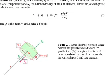
Figure 2.Graphic illustration of the balance between the pressure force (FP) and the
gravity force (Fg) on a given infinitesimal
element at distance r from the center of the star with tickness dr and base area dA.
This is a simple example of EoS; however in most cases it’s not far from the reality; for the Sun and solar like stars the law of perfect gas holds with a very good approximation, except for the very central regions in which few percents of the pressure are due to degenerate electrons.
The most of the stars are at mechanical (hydrostatic) equilibrium. This means that at each point inside a star, the pressure counteracts the gravity force which would cause the stellar contraction (see Fig. 2). The gravity is a central force, thus the equilibrium configuration is a sphere. This simplifies very much the calculations: for spherical symmetry all the quantities can be expressed as a function of one variable e.g. the radial coordinate. Thus one assumes a stellar structure composed of several spherical shells so thin that the physical quantities inside each shell can be considered as constant. Under this assumption the massdMinside each shell of radiusdris given by:
dM(r) =4πr2ρ(r)dr, (2)
whereρ(r)is the corresponding density inside the shell. This is called “continuity equation”. By equating for each shell inside the star the gravity force and the pressure force (gas + radiation pressure) one obtains the so called “hydrostatic equilibrium equation”:
dP(r)
dr =−
GM(r)ρ(r)
r2 , (3)
The two equations written until now, as a function of the radius, contains three unknowns: P(r),ρ(r) and M(r). P(r) andρ(r) are linked through the equation of state, but, except some particular EoS, also the temperature (unknown) appears in the EoS. Thus the system of equa-tions is still not resolvable. This is expected, because one still has to take into account the energy production and transport, which play an important role in stellar structures.
Stars lose energy from the surface (mainly) due to photon emission. The whole star is in thermal equilibrium that is the amount of energy per unit time (luminosity) which exits from a given shell direct outward is equal to the amount of energy which enters in the shell plus the energy possibly produced in the shell itself. The mechanisms of energy production active in stars are: nuclear reactions, thermodynamic transformations of the gas linked to contractions and expansions of stellar regions (the so called “gravitational energy”) and neutrino energy losses. Neutrinos have a mean free path larger than the stellar radius (except the case of very dense stellar nuclei of massive stars at the end of their life) and thus they escape from the stars without interacting with the stellar matter, that is without releasing their energy to the stellar structure.
Stellar interiors are so hot (temperatures higher than about 6·106K) that fusion nuclear reactions of nuclei to form heavier elements can happen. In stars the most of fusion reac-tions happen among thermalized charged nuclei of the stellar plasma screened by the plasma electrons (see e.g. Ref. [3] or other talks at this school for a description of nuclear fusion mechanisms in stars). It’s worth to remind that the higher is the charge of reacting nuclei the higher is the threshold temperature for the ignition of the fusion.
Usually we define ε the energy produced/lost per unit time and unit mass due to the mechanisms described above, that is: ε=εnuclear+εgravitational−εneutrinos. Each process of energy production depends on the physical quantities (density/pressure and temperature) and chemical composition which vary at each point of the star. The thermal equilibrium equation in each shell of the star can thus be expressed as:
dL(r) dr =4πr
2ρ(r)ε(r), (4)
where L(r) is the luminosity which enters in the shell of radius r.
Another equation is added to the system but another unknown, i.e. L(r), is also added. The energy produced in the internal regions must be transported across the whole star. The only energy transport mechanism which is always active in stars is the radiative trans-port, that is the totality of processes of photon-matter interaction (photon electron scattering, photoionization, inverse bremsstrahlung, photon absorption, and further isotropic emission, of photons by atoms, etc). Under specific conditions electronic conduction and convection (matter elements which move from hotter to colder regions releasing their heat) can also be active.
In general, the precise treatment of the interaction phenomena between radiation and matter and of the transport of energy by radiation is a very complex task. However the fact that photons follow a Planck distribution allows to adopt a simplified description, whose results agree with those of the more complete theory in the limit of a very short mean free path of the photons.
it’s possible to define the radiative opacity coefficient (krad) as:
krad= 1
ρλp,
(5)
whereλpis the photon mean free path andρ the mass density. krad has the dimension of a cross section (of the various photon-matter interaction processes) per unit mass, and it’s typically expressed in cm2/g. It’s useful to remind thatk
rad is stronger when matter is not completely ionized.
The diffusion approximation holds since photons perform a random motion, interacting with particles after having covered a mean free path. By assuming that the photon-matter interaction is the only active energy transport mechanism, it is easy to find (see e.g. Chapter 3 of Ref. [4]) a relation between the temperature gradient (radiative gradient) and the energy flux to be transported, the so-called “energy radiative transport equation”:
dT(r)
dr =−
3 4
krad(r)ρ(r) ac
1 T(r)3
L(r)
4πr2 , (6)
which holds at each radial coordinate,r, of the star.
If the temperature gradient required to a stellar structure to transport all the energy through photon-matter interactions would be too much high, energy transport through convection becomes efficient too, even if radiative transport is still present. If convection is efficient, hotter and relatively light elements of fluid rise, while cooler and relatively heavy elements sink. Then the elements are dissolved and the gas is mixed. As a result, the rising elements deposit their excess heat to the surroundings leading to a net transport of energy in the external direction (obviously the sinking elements similarly contribute to the energy transport). In this case the temperature gradient is no more the radiative one.
The motion of convective elements is extremely difficult to describe, due to the turbu-lence and viscosity of the gas. Thus the precise determination of the convective flux and the temperature gradient in stellar convective regions can be very difficult. Luckily, this is not a problem in the stellar interiors, when the density is enough high; in this case, the local temperature gradient can be approximated with a very high precision through the adiabatic one. The situation is different in the external envelopes, where the matter density is much lower; in this case precise hydrodynamic calculations should be needed which however, due to the computational complexity of the simulations, are available only for small fractions of selected stellar structures and never cover a complete stellar evolutionary sequence.
Given this situation semi-empirical approaches are generally adopted in the external con-vective envelopes; the most largely used is the Mixing Length Theory (MLT) [5] in which the convection efficiency is parameterized in terms of the mean path travelled by the up-ward/downward moving matter (the so-called mixing length, l). l cannot be obtained “a priori” in this scheme but it’s assumed to be a multiple of the pressure scale length (HP), i.e. the path along with the pressure is decreased by 1/e. We can thus write: l=αmlHP, where
αml is a free parameter (mixing length parameter) which must be tuned to obtain agreement with stellar observables. In fact, the temperature gradient in the stellar convective envelope determines the effective temperature and, thus, the stellar radius at fixed luminosity. In sum-mary, the present stellar physics theory is still not able to model in a precise way convection in stellar external parts; this leads to an uncertainty in the predicted stellar radius for stars with external convective envelopes. This uncertainty however is not expected to affect in a significant way the stellar luminosity.
the local energy production, opacity and EoS. Thus stellar models are the results of calcu-lations relying on the adopted input physics (e.g. EoS, radiative and conductive opacities, nuclear reaction rates, etc..) and the assumed original chemical composition for the star. Each of these ingredients is affected by not negligible errors and thus stellar models are still affected by significant uncertainties. For more details about stellar structures see e.g. the books by Refs. [4], [6] and [7].
3.6 3.62 3.64 3.66 3.68 3.7 3.72 3.74
LogTeff -0.75
-0.5 -0.25 0 0.25 0.5 0.75
logL/L
O
TO
PMS
PMS MS
M=0.75 MO
Figure 3.The evolution in the HR diagram of a 0.75Mstar from the PMS to the central H exhaustion (Turn off, TO).
3 Pre-Main Sequence and Main Sequence stars
Stars born inside a molecular cloud of gas and interstellar dust; the gas is mainly composed by H and He with traces of other elements. These molecular clouds, neglecting, as a first ap-proximation, possible effects due to rotation and magnetic fields, are in equilibrium between the gravitational force and the pressure force. However, due to stochastic motions, the colder and more dense regions of the cloud can start to contract. As soon as the collapse proceeds the region fragments more and more until each part in which the original region of the cloud has been divided will form a star.
It’s well known that the stars can exist only in a limited range of masses. Objects with masses lower than≈0.08M(the precise value depends on the chemical composition) do not succeed to ignite hydrogen (see following discussion), while the upper mass limit for stellar stability is still not defined with precision. For a long time, observations favored a present-day upper stellar mass limit around 150÷200 M; the original mass can be higher because in these massive stars strong mass losses through stellar winds are expected. However it’s not clear whether the apparent observed upper limit simply represents a statistical limit owing to a lack of sampled very massive stars in stellar clusters.
most of the choices about mass accreting parameters (accretion rate, accretion history, etc..) and accretion geometry for the proto-star, even if there is not complete agreement about these conclusions.
During the proto-stellar phase the star contracts and warms up until the achievement of the hydrostatic equilibrium: the gas force exactly counterbalances the gravity force. The stellar gas pressure is mainly due to its temperature. However the star is warm and radiates, losing energy from the surface; thus, after a while, the star cools down and its pressure decreases becoming insufficient to completely sustain the star against the gravity. The star slightly contracts increasing its temperature and reaching again the hydrostatic equilibrium until the radiation losses from the surface cools down again the star. The PMS phase is characterized by these consecutive stellar contractions when the star passes from one “equilibrium” state to another one, while its internal temperature increases. The timescale of these processes is the one at which the stars cools down (thermal timescale also called “Kelvin-Helmholtz” time) which varies with the stellar mass in the range of 106-107years. In the first PMS phases stars are expected to be fully convective; thus they are completely mixed and possible chemical inhomogeneities of the original cloud are canceled.
While the star contracts being fully convective its density increases too and the radius sig-nificantly decreases, then also the luminosity strongly decreases. During this fully convective phase stars evolve in the HR diagram along an almost vertical line i.e. at approximately constant effective temperature, the so called “Hayashi track”, see Fig. 3. As soon as the tem-perature in the central regions grows, the corresponding opacity decreases; thus a radiative core forms and grows, surrounded by an external convective envelope, whose mass decreases more and more with the correspondingly increase of the radiative core. All the stars which de-velop a radiative core leave their Hayashi track, when the radiative core extension increases, and move towards higher effective temperatures (to the left of the Hayashi track in the HR diagram). When a sizable radiative core is established, the star moves almost horizontally in the HR diagram with a constant increase of the central temperature due to contraction.
Eventually, most of the stars reach the temperature for H-burning into helium in the core, the warmest region of the star. The hydrogen fusion into helium is the first nuclear reaction able to produce an energy which can counterbalance the radiative losses from the surface. Hydrogen is the first abundant element to be burned, because the Coulomb barrier for the fusion of two protons is the lowest one, and hydrogen is the most abundant element in the Universe.
When hydrogen fusion is fully active, the star is in equilibrium, with the nuclear reactions which supply to the star the energy lost by photon emission from the photosphere.
phase, the stellar luminosity is mainly due to the stellar mass (with a weaker dependence on the chemical composition). It is exactly when center H burning is so efficient to counterbal-ance the energy losses from the surface, that the star leaves the PMS phase and starts its MS evolution1.
The name “Main Sequence” is due to the fact that stars in this phase occupy in the HR diagram a mono-parametric sequence (at fixed chemical composition), whose parameter is the stellar mass. The star is now in equilibrium, thanks to the nuclear energy, but the reaction efficiency decreases according to the reduction of the fuel (hydrogen) abundance. Thus, after a while, the nuclear energy is no more enough to counterbalance the radiative losses and the star contracts again, with the timescale of the fuel abundance reduction, that is of the nuclear burning rate. Therefore, the temperature of the central regions slightly increases until the energetic equilibrium is reached again, with a slightly different configuration of the stellar structure: the star evolves following a nuclear timescale.
Nuclear timescales strongly vary with the stellar mass; the higher is the mass, the higher is the luminosity and thus the higher is the rate of the nuclear reactions which counterbalance the energy losses due to radiation. Moreover, the higher is the fusion rate, the lower is the time in which the fuel is exhausted. To be more precise, for most of the stars (but the most massive ones) the luminosity increases with the mass,M, asMθ, withθ=2.5÷4.5, while the H-abundance linearly increases withM. As an example the Sun will take about 10 Gyr to consume the hydrogen in its central regions, while a 15 Mstar of the same chemical composition will take about 107years.
The reduction of fuel, during central H-burning, leads to slight variations of the stellar characteristics; a general feature during central H-burning is that stars increase their luminos-ity (see Fig. 3).
Hydrogen burning can be represented symbolically by the “fusion” reaction: 4p + 2e− → 4He+ 2νe. The total energy released is Q≈26.73 MeV, whose only a small part (about 0.6 MeV) is carried away by the two electron neutrinos, while the remaining is available to the stellar structure. From the solar radiative flux at the Earth (solar constant K=8.533(1±0.004)·1011MeV cm−2s−1[9]) one immediately derives the total flux,Φtot, of electron neutrinos arriving on the Earth, if they are not losten route(by neglecting the small fraction of energy carried by neutrinos):
Φtot≈2K/Q≈7·1010cm−2s−1 . (7)
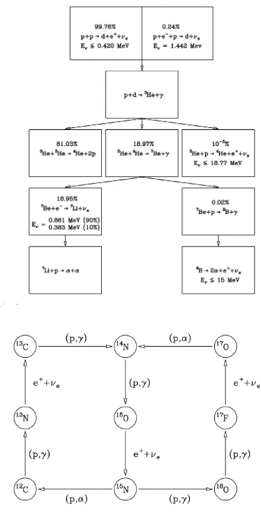
Two different sets of reactions could convert enough hydrogen into helium to provide the energy needed for the stellar luminosity, namely the proton-proton (pp) chain and the CNO bi-cycle, whose reactions are sketched in Fig. 4. Due to the different Coulomb barriers of the two groups of reactions, the mean temperature dependence of the reaction rate, r, (r∝Tβ) varies. β is≈ 4 for the pp chain while the CNO bi-cycle, which include reactions with heavier nuclei, has a stronger temperature dependence ofβ≈17. Remembering that the internal temperatures increase with the stellar mass one can thus understand why Main Sequence stars with masses lower than about 1.2 M(for solar chemical composition) burn H mainly through the pp chain while in higher masses the CNO bi-cycle dominates (see e.g. Ref. [3] for more details).
Eventually the star consumes the hydrogen in the central region in which H burning can be efficient; the central H exhaustion is easily identified in the HR diagram with the maximum in effective temperature (see Fig. 3). The history of a star after the central H-exhaustion can be roughly seen as a succession of central burnings of elements with charges higher and
1More precisely, the MS phase starts when central H nuclear fusion completely counterbalances the energy
Figure 4. Upper panel: the pp chain. The probability of the different branches is indicatively the one of the solar model. The neutrino energies, Eν, are also indicated. Lower panel: sketch of the reactions of the CNO bi-cycle.
4 Solar models
One of the most important test for stellar evolutionary theories is clearly our Sun, the closest and best studied star; the challenge is to theoretically reproduce the various observational information. Following the definition proposed by John Bahcall in 1995 a “Standard So-lar Model (SSM)” can be described as the one which reproduces, within uncertainties, the observed properties of the Sun, by adopting a set of physical and chemical inputs chosen within the range of their indeterminacy. On the contrary to what happens for the most of other stars, the Sun mass, radius, and luminosity are known with great accuracy. They are respectivelyM=1.98892(1±0.00013)×1033g ,R
=6.9599(1±0.0001)×1010cm and L=3.8275(1±0.0014)×1033erg/s [10]. The effective temperature is related toR
and Lthrough the black body relation, and one findsTe,=5772.0±0.8 K [10]. The Sun age, estimated through radioactive dating of meteorites, ist=4.57(1±0.0044)Gyr [9]. In as-trophysics the fractional abundance in mass of hydrogen, helium and elements heavier than helium (called “metallicity”) are indicated, respectively, withX,Y andZ; thusX+Y+Z=1. The solar metallicity is essentially dominated, in order of importance, by oxygen, carbon, neon, nitrogen and iron. The present ratio of heavy elements to hydrogen in the photosphere, following Ref. [11], is(Z/X)photo = 0.0180, even if this quantity is still under debate (see following discussion).
If a complete information about the (initial) photospheric composition is available and if the theory of stellar models is able to predict with precision stellar radii the theoretical models should account for the solar luminosity and radius at the solar age, without tuning any free parameter. However a direct evaluation of the solar surface helium abundance is not available and the determination of the present solar surface abundance of various elements is still un-certain. Moreover, the present observed photospheric composition is different from the initial one, due to the effect of microscopic diffusion (mainly gravitational settling) whose efficiency is estimated to be known with a precision not better than about 15% [12]. In addition, evo-lutionary models clearly show that the solar interior is largely radiative, while a convective envelope occupies about the outer 30% of the solar radius. The top of the convective cells, which reach the phosphere, can be observed as “solar granulation”. As discussed in Sec. 2, theoretical predictions of radii for stars with convective envelopes are affected by significant uncertainties and a semi-empirical parametrization for the external convection efficiency is generally used. Thus, one has the freedom of adjusting some parameters in the course of the calculation.
To produce a SSM, one evolves an initially chemically homogeneous solar mass up to the Sun age. To obtainL,R, and(Z/X)photoat the solar age, one can tune three parameters: the initial helium abundanceY, the original metal abundanceZ, and the convection efficiency, through the mixing length parameterαml. The effects of the above mentioned parameters on solar models can be simply understood. The luminosity of main sequence stars, and thus of the Sun too, depends also on the initial helium contentY; increasing it, the initial Sun is hotter and thus brighter and its evolutionary time is then shorter. Since the originalZ/Xratio is constrained by the requirement to fit the present photospheric abundance,Y andZcannot be chosen independently: ifY increases,Z must decrease. The effect of the original helium abundance on stellar radius is much less important.
It’s worth noticing that, just like any other stellar model, a SSM depends on a number of input parameters which have been refined with time but are still affected by not negligible uncertainties.
Thus, to reproduce only the observational values forR,Land(Z/X)photoat the esti-mated solar age the model depends on three (essentially) free parameters, i.e.αml ,Y, and the original(Z/X)value. This may not look as a so big accomplishment. At this level, the confidence in SSMs actually rests on the success of stellar evolution theory to describe many, and more complex, evolutionary phases in good agreement with observational data.
However, helioseismology added important data on the solar structure, which provide se-vere constraints on SSM calculations. Roughly speaking, the Sun (as the other stars) supports an enormous amount of oscillation modes around its position of stable equilibrium, whose oscillation frequencies can be observed with a very high precision. The observed oscilla-tion spectrum can be derived from the Doppler shifts of photospheric absorposcilla-tion lines. The quantities we are interested in are the so-called “eigenmodes”, i.e. standing waves. The res-onant cavity of these modes has its outer boundary in the solar atmosphere, but the location of the inner boundary depends on the characteristics of each individual mode, frequency and angular degree. As a result, different modes map the Sun to different depths and allow to determine the physical properties of the internal structure as a function of depth.
In particular, helioseismology can accurately determine the sound speed profile inside the Sun, the depth of the convective zone and the present photospheric helium abundance (see Ref. [13] for an extended review about helioseismology). If one takes into account helioseismic results, there are essentially no free parameters for SSM builders. The goal is to obtain the so-called “solar seismic model”, i.e. a model which also satisfies the helioseismic constraints (see Fig. 5 for the predicted sound speed).
0 0.1 0.2 0.3 0.4 0.5 0.6 0.7 0.8 0.9 1
R/Rtot
0.0e+00 5.0e+14 1.0e+15 1.5e+15 2.0e+15
P/
ρ
Standard Solar Model
c2= P/ρ
=5/3 for R/Rtot < 0.95
Figure 5.The P/ρbehaviour (proportional to the sound speed squared) predicted by the Standard Solar Model. The change in the slope, indicated by the arrow, marks the position of the bottom of the external convective envelope.
zones and fusion efficiency through the CN-NO bi-cycle. As a consequence, also the origi-nal helium abundance estimation changes together with the predicted dept of the convective envelope, which becomes shallower.
Several authors pointed out a disagreement between the observed and the predicted sound speed, mainly near the bottom of the convective envelope, for models with the revised chem-ical composition together with a too low surface helium abundance and a too shallow con-vective envelope. Thus, it can be reasonably assumed that SSMs match the Sun only to a few percent. Due to the quoted very high precision of the seismic results, these discrepancies, even if small, are statistically significant.
Moreover the present estimated original solar helium abundance appears quite low, Y ≈ 0.250 ÷ 0.265 with respect to the estimates with “older” solar mixtures and this could constitute a problem for chemical galactic evolution studies. During their evolution stars produce helium and metals through nuclear fusions; these elements are then casted into the interstellar medium by stellar winds and stellar explosions, increasing their mean Galac-tic abundance. Considering the present quoted value for the primordial helium abundance (YP≈0.247) [16]) the adoption of a low solar helium abundance would lead to a quite low estimate for theΔY/ΔZ enrichment with respect to present independent evaluations of this quantity in the Milky Way (ΔY/ΔZ≈1÷5 ) , see e.g. Ref. [17].
Many possible solutions have been put forward to explain the problem, which however is still open, constituting the so called “solar abundance problem”. Each of the solution proposed in the literature (increased opacity below the convective zone, increased neon abun-dance, etc..) mitigates the discrepancies without completely eliminating them. Moreover, the required change in the quoted quantities exceeds the likely uncertainties in existing input data. Recently direct measurements of intrinsic opacities were made under conditions re-sembling those at the base of the Sun’s convection zone showing that the intrinsic opacity of iron was higher than expected, leading to an increase of the total opacity of about 7%, while the chromium and nickel opacity calculations seem to agree with experimental data (see e.g. discussion in Ref. [18]).
Regarding solar neutrino production, at the temperature and density characteristic of the solar interior (T ≈107K,ρ ≈150 g/cm3), hydrogen burns with the largest probability (≈98%) through the pp chain, even if a minor production of CNO neutrinos is also present. After the solution of the “solar neutrino problem” thanks to the results of the SNO experiment (see e.g. discussion in Ref. [19]) solar neutrinos can be used to test the goodness of the solar model predictions. Solar neutrino fluxes can be inferred from global fits to solar neutrino experimental data in the neutrino flavour oscillation framework, with the constraint that the sum of the thermal energy generation rates associated with each of the solar neutrino fluxes coincides with the solar luminosity (see e.g. discussion in Ref. [20]). Present experimental results are in agreement with solar models predictions in the neutrino flavor oscillation framework and within theoretical and experimental uncertainties (independently if the “old” or the updated solar chemical composition is assumed). Thus, at present, solar neutrino data cannot help to solve the solar abundance problem, but further improvements in experimental determination of solar neutrino fluxes (in particular of the less abundant CNO neutrinos) could change the situation. For more information about these arguments see e.g. Ref. [21].
References
[1] L. Girardi, G. Bertelli, A. Bressan, C. Chiosi, M.A.T. Groenewegen, P. Marigo, B. Salasnich, A. Weiss, A&A391, 195 (2002)
[2] Gaia Collaboration, A&A616, A10 (2018)
[3] C.E. Rolfs, W.S. Rodney,Cauldrons in the cosmos: Nuclear astrophysics(University of Chicago Press, Chicago, 1988)
[4] M. Salaris, S. Cassisi,Evolution of Stars and Stellar Populations(Wiley-VCH, 2006) [5] E. Böhm-Vitense, Zeitschrift fur Astrophysik46, 108 (1958)
[6] J.P. Cox, R.T. Giuli,Principles of stellar structure (New York, Gordon and Breach, 1968)
[7] C.J. Hansen, S.D. Kawaler, V. Trimble,Stellar interiors : physical principles, structure, and evolution(Springer-Verlag, New York, 2004)
[8] S.W. Stahler, F. Palla,The Formation of Stars(Wiley-VCH, 2005)
[9] J.N. Bahcall, M.H. Pinsonneault, G.J. Wasserburg, Reviews of Modern Physics67, 781 (1995)
[10] A. Prša et al., Astronomical Journal152, 41 (2016) [11] M. Asplund et al., ARAA47, 481 (2009)
[12] A.A. Thoul, J.N. Bahcall, A. Loeb, ApJ421, 828 (1994)
[13] J. Christensen-Dalsgaard, Reviews of Modern Physics74, 1073 (2002) [14] A.M. Amarsi, M. Asplund, MNRAS464, 264 (2017)
[15] E. Caffau et al., Sol. Phys.268, 255 (2011) [16] C. Pitrou et al., Phys. Rep.754, 1 (2018)
[17] M. Gennaro, P.G. Prada Moroni, S. Degl’Innocenti, A&A518, A13 (2010) [18] S. Basu, Physics Online Journal12, 65 (2019)
[19] A. Bellerive et al., Nuclear Physics B908, 30 (2016)
![Figure 1. Color-Magnitude Diagram of the Gamma Velorum stellar cluster in the Gaia photometricbands, data from the Gaia Collaboration (see [2]).](https://thumb-us.123doks.com/thumbv2/123dok_us/7985741.1324980/2.482.88.390.224.372/figure-magnitude-diagram-velorum-stellar-cluster-photometricbands-collaboration.webp)