On the Leakage Resilience of Ring-LWE Based
Public Key Encryption
Dana Dachman-Soled, Huijing Gong, Mukul Kulkarni, and Aria Shahverdi
University of Maryland, College Park, USA
danadach@ece.umd.edu, gong@cs.umd.edu, {mukul@terpmail, ariash@terpmail}.umd.edu
Abstract. We consider the leakage resilience of the Ring-LWE analogue of the Dual-Regev encryption scheme (R-Dual-Regev for short), originally presented by Lyubashevsky et al. (Eurocrypt ’13). Specif-ically, we would like to determine whether the R-Dual-Regev encryption scheme remains IND-CPA secure, even in the case where an attacker leaks information about the secret key.
We consider the setting whereRis the ring of integers of them-th cyclotomic number field, formwhich is a power-of-two, and the Ring-LWE modulus is set toq≡1 modm. This is the common setting used in practice and is desirable in terms of the efficiency and simplicity of the scheme. Unfortunately, in this settingRq is very far from being a field so standard techniques for proving leakage resilience in the general lattice setting, which rely on the leftover hash lemma, do not apply. Therefore, new techniques must be developed.
In this work, we put forth a high-level approach for proving the leakage resilience of the R-Dual-Regev scheme, by generalizing the original proof of Lyubashevsky et al. (Eurocrypt ’13). We then give three instantiations of our approach, proving that the R-Dual-Regev remains IND-CPA secure in the presence of three natural, non-adaptive leakage classes.
1
Introduction
Side-channels allow attackers to bypass the security of a cryptosystem by exploiting implementation-specific properties. Attackers can recover cryptographic keys through physical measurement of various aspects such as execution time, power consumption, or even sound waves generated by the processor. Such attacks are known to be detrimental against standard cryptosystems, such as RSA, and can be launched with reasonable costs in myriad settings (cf. [4,16,24,25,22,41,38,18]). The emergence of these attacks has prompted cryp-tographers to incorporate side-channels in formal security models and to constructleakage resilient schemes that remain secure in these enhanced models. There is a large body of work on leakage-resilient cryptography (cf. [17,2,33,6,26,23], to name just a few). Moreover, several seminal works including [20,2,15,13] focus on constructing/analyzing leakage-resilientlattice-based cryptosystems.
Among cryptosystems built from lattices, so-called ring-based schemes are usually preferred in practice, since these highly structured rings lend themselves to more efficient and compact cryptosystems. Unfortu-nately, the current techniques for obtaining leakage resilience in the general lattice setting crucially rely on the fact that the public key matrix A is a random matrix 1 and therefore do not carry over to the ring setting. This leaves open the question of whether we can enjoy the efficiency of ring-based cryptosystems, while simultaneously achieving leakage resilience.
Leakage-Resilient Post-Quantum Cryptography. One of the foremost avenues for viable post-quantum public key cryptography is to construct schemes from ideal lattices. Currently 12 submissions out of 69 submission for first round of NIST submissions are ring-based. The goal of our work is to analyze the leakage resilience of a post-quantum, public key encryption scheme with practical parameter settings (i.e. focusing on the ring setting and requiring at most a small constant number of ring elements in the public key). Specifically, we analyze security of the Ring-LWE analogue of the Dual-Regev encryption scheme (R-Dual-Regev for short),
1
For example, techniques include decomposition of the matrixAinto two random matrices of varying dimensions [2] and/or using the fact thatATxis a strong randomness extractor whenA∈Zm×n
first presented by Lyubashevsky et al. [28] and then simplified by Alperin-Sheriff and Peikert and Crockett and Peikert [3,11].
Lattices and LWE. An n-dimensional lattice L is an additive discrete subgroup of Rn. There are several algorithmic problems relating to lattices that are believed to be hard, even for a quantum computer. The relevant one for this work will be the (approximate) shortest independent vector problem (SIVPγ), which asks to find a set ofn linearly independent vectors (wherenis the dimension of the lattice) such that the length of the longest vector in the set is within aγ factor of the minimum possible length.
The learning with errors (LWE) problem was introduced by Regev [37], who showed a worst-case to average-casequantumreduction fromSIVPγ.2To solve the (decision version of the)LWEproblem, an attacker must distinguish the two distributions (A, Ax+e) from (A,u), whereA is a matrix chosen uniformly from
Zqm×n, x is sampled from Zqn, e is sampled from an “error distribution” ψm over Zqm and u is chosen uniformly from Zm
q . Many lattice-based public-key encryption schemes are built from LWE (following the original construction of [37]) and the security is proven by first reducing lattice problems toLWE and then reducingLWEto these schemes. (cf. [19,8]).
Ideal lattices and Ring-LWE. When using the LWE assumption over general lattices to build encryption schemes, the public key consists of the LWE matrixA, a random matrix overZq of sizem×n, wherem≥n and n is security parameter. So storing the public key requires space at least Ω(n2logq), and encryption requires matrix-vector multiplication. To over come this inefficiency,ideal lattices—lattices with additional structure—were introduced. In the ideal lattice setting, we consider the number fieldK=Q[x]/Φm(x), where
Φm(x) is them-th cyclotomic polynomial of degreeϕ(m). Formwhich is a power of 2, them-th cyclotomic polynomial is simply Φm(x) = xn+ 1, where n =m/2 is also a power of 2. We then consider the ring of integers,R⊂Kof the number field, defined asR=Z[x]/Φm(x).Rcan now be viewed as a lattice via the so-called “canonical embedding” which transforms elements ofKfrom a polynomial representation to a vector representation in an inner product space endowed with a vector norm. “Ideal lattices”, therefore, correspond to fractional ideals of K, which can be viewed as lattices via the canonical embedding. We further define
Rq :=Zq[x]/Φm(x), which denotes the set of polynomials obtained by taking an element ofZ[x]/Φm(x) and reducing each coefficient moduloq.
Given the above, the Ring-LWE problem is to distinguish (a, b =a·s+e)∈ Rq×Rq from uniformly random pairs, wheres∈Rq is a random secret, thea∈Rq is uniformly random and the error terme∈R has small norm.
In the above formulation, the matrixAfrom the general lattice LWE setting is replaced with a polynomial
ain the ring setting. Therefore, the public key now has dimensionninstead ofm×nand can be represented as a vector inZn
q, requiring onlyO(nlogq) bits of storage.
In this paper, we consider rings with further structure. Specifically, we assume that mis a power of two, which means thatΦm(x) has degreen=m/2. We further set q to be a prime such thatq≡1 modm, in which case Φm(x) completely splits into n factors in Zq[x]. This allows for additional optimizations in the implementation, such as fast arithmetic over the ringRq.
The R-Dual-Regev encryption scheme. The key generation algorithm of the R-Dual-Regev encryption scheme proceeds as follows: The secret key corresponds to elementsx1, . . . , xlthat are chosen from a discrete Gaussian distribution overR. To generate the public key,a1 is set to−1∈Rq anda2, . . . , al are chosen uniformly at random fromRq. The public key is then set to (a2, . . . , al, al+1=−Pi∈[l]aixi). The key property necessary for proving the security of the Dual-Regev encryption scheme is that for public keys sampled as described above,al+1 should be distributed (close to) uniform random inRq, givena2, . . . , al.
WhenRq is a field, not only does the above property hold, but it can be shown that al+1 is distributed (close to) uniform random inRq, as long asx1, . . . , xlhas sufficiently high min-entropy (via the leftover hash lemma). Thus, whenRq is a field, it can be immediately argued that the R-Dual-Regev encryption scheme is inherently leakage-resilient, to (non-adaptive) leakage3 on the secret keyx
1, . . . , xl, as long asx1, . . . , xlhas sufficiently high min-entropy conditioned on the leakage. This would allow to argue, in particular, that the
2 Classical reductions fromGapSVPwere subsequently proved by Peikert [34] and Brakerski et al. [7]. 3
scheme is leakage resilient against any leakage function with bounded output length. In this work, however, recall that we consider the case where R is the ring of integers in the mth cyclotomic number field K of degreen, wherem is a power-of-two, and the modulusq is a prime such thatq≡1 modm. As discussed above, such setting of parameters is desirable since it allows for highly efficient implementation of various aspects of the cryptosystem (such as discrete Gaussian sampling, as well as representation and manipulation of elements ofRandRq). Unfortunately, whennandqare chosen as above, it implies thatqR(the ideal of
Rgenerated byhqi) splits completely intondistinct prime ideals,p1, . . . ,pn, each of normq, which in turn means thatRq is very far from being a field. In particular, this means that standard techniques for proving leakage resilience, which rely on the leftover hash lemma, cannot be used when computing over the ringRq. Indeed, a result analogous to the leftover hash lemma, proving thatal+1is indistinguishable from random, given a constant fraction of leakage on the secret key, is impossible in the setting discussed above. For example, if the adversary learns thei-th NTT coordinate of each ring element in the secret key x1, . . . , xl, then the
i-th NTT coordinate ofal+1=−Pi∈[l]aixi is known4, and soal+1is very far from uniform. Yet this is only a 1/nleakage rate!5
Nevertheless, Lyubashevsky et al. [28,29] proved a “regularity theorem” showing that (even when q is a prime such that q ≡ 1 modm) for matrix A = [Ik|A¯] ∈ (Rq)
k×l
, where Ik ∈ (Rq) k×k
is the identity matrix and ¯A ∈ (Rq)
k×(l−k)
is uniformly random, and x chosen from a discrete Gaussian distribution (centered at 0) overRl
q, the distribution overAxis (close to)uniform random. A similar result was proven by Micciancio [31], but requires super-constant dimension l, thus yielding non-compact cryptosystems. In contrast, the regularity theorem of [28] holds even for constant dimension l as small as 2, and thus yields compact cryptosystems. However, while sufficient for proving the security of the cryptosystem itself, unlike the more general leftover hash lemma, the statement of the regularity theorem of [28] implies nothing about the security of the cryptosystem in the leakage setting. To prove the security of the R-Dual-Regev encryption scheme under leakage, we extend the regularity theorem to settings in whichxis chosen from a distribution D, which is not necessarily a Gaussian distribution centered at 0. Specifically,Dcorresponds to a Gaussian distribution conditioned on the leakage obtained on the secret key x. I.e. D corresponds to the distribution of the secret key from the leaking adversary’s point of view. Thus, the fundamental technical question we consider in this work is:
For which distributionsDoverx∈Rlq, whereR,qare as above andlis constant, is the distribution overAx(close to)uniform random, forAas above?
We make progress on the fundamental question above and show that for three natural classes of leakage— which give rise to three different distributionsD—whenxis sampled according to D, the distribution over
Axremains (close to) uniform random. This implies that the R-Dual-Regev encryption scheme is resilient to these three types of leakage (with possibly small modifications to the scheme such as increasing the standard deviation of the Gaussian distribution under which the secret keyxis sampled during key generation).
1.1 The Leakage Scenarios
In the following, we describe the three leakage scenarios considered in this work.
Leakage Scenario I. Recall that the secret key of the R-Dual-Regev encryption scheme is x= (x1, . . . , xl), where each xi ∈Rq. Moreover, eachxi itself is represented as ann-dimensional vector. Thus, in total, the secret key can be viewed as anl·n-dimensional vector. This attack scenario captures an adversary who uses a fast, but inaccurate device to obtain noisy measurements of each sampled coordinate of the secret key (e.g. through a power or timing channel). Specifically, independent Gaussian noise with standard deviation at leastsis added to each leaked coordinate, wheresis the standard deviation of the Gaussian distribution from which the secret key,xis sampled.
4
Applying the NTT transform to ring elementsai, xi∈Rq—resulting inn-dimensional vectors,bai,bxi∈Z
n
q—allows forcomponent-wisemultiplication and addition, so thei-th NTT coordinate all values ofaixiwill be known, given the leakage and thus thei-th NTT coordinate ofal+1 is known.
5
Leakage Scenario II. As above, we consider a side-channel attack that is launched during the sampling of the secret key. Now, the attacker has a slower, but more accurate device which allows it to obtain more accurate measurements for aconstant fraction of the coordinates of the secret key, but no information for the remaining coordinates. In this scenario, the noise added to each leaked coordinate has only 2nstandard deviation.6 In comparison, in Leakage Scenario I the standard deviation of the noise is at least s, where
s is the standard deviation of the Gaussian distribution from which the secret key, x is sampled. When instantiating the R-Dual-Regev encryption scheme withq=Θ(n3) andl= 5,sis at least n1.6.
Leakage Scenario III. In this scenario, the adversary learns the magnitude of the secret key with channel error, where both secret key and error are sampled from Gaussian distributions. The motivation for this type of leakage is that (discrete) Gaussian sampling of the secret key is often implemented via rejection sampling in practice [12,7]. Briefly, in rejection sampling we have a distribution D0 that is sufficiently close to the target distributionD (i.e.D(x)≤M ·D0(x), where D(x), resp.D0(x), denotes the probability of xunder
distributionD, resp.D0). We samplexaccording toD0, outputxwith probabilityp= MD·D(x0()x)and reject with
probability 1−p. In case of rejection the procedure is repeated. In our setting,D0 can correspond to a multi-dimensional binomial distribution (with parameters set such that the one-multi-dimensional binomial distribution is 1−δ-close to the one-dimensional Gaussian distribution), for which sampling is straightforward. The probabilitypof accept depends on the probability ofxunder the Gaussian distribution,D(x), which in turn depends only on themagnitudeofx.7Our result suggests that it may be better (from a security perspective) to sample the entire xfrom a multi-dimensional distribution D0 and then apply rejection sampling to the entire vector at once, as opposed to performing the rejection sampling coordinate-by-coordinate, since in this case there is only one opportunity for leakage.8.
1.2 Our Results
We show that in each of Leakage Scenarios I, II and III, the R-Dual-Regev encryption scheme can be proven secure, as long as the parameter s—corresponding to the standard deviation of the Gaussian from which the secret key is sampled—is slightly increased. Specifically, in the original analysis of the R-Dual-Regev encryption scheme by Lyubashevsky et al. [28], it was shown that it is sufficient to sets≥2n·q1/l+2/(nl), wheren is the dimension,qis the modulus andl is a constant representing the number of ring elements in the secret key, public key and ciphertext. We next describe the setting ofsin each of the leakage scenarios:
– For Leakage Scenario I, we show that it is sufficient to set s≥√2·2n·qk/l+2/(nl), an increase of a multiplicative factor of√2. (see Theorem5.2, Corollary5.3and the discussion following the corollary).
– For Leakage Scenario II, we show that it is sufficient to sets ≥2n·qlkn(n−+2`), where ` is the number of leaked coordinates of the secret key. (see Theorem5.4, Corollary 5.8and the discussion following the corollary). Surprisingly, even if leaked coordinates of secret key x have standard deviation 2n, which is significantly smaller than smoothing parameter of the lattice Λ⊥(A)—which is 2n·qk/l+2/(nl) (see Theorem 3.13)—distribution ofal+1=−Pi∈[l]aixi can still be (close to) uniform random.
– ForLeakage Scenario III, we show that it is sufficient to sets≥p
14/5·(n0/n)·lnn0·2n·qk/l+2/(nl), where n0 =n·l+ 1, an increase of a multiplicative factor ofp14/5·(n0/n)·lnn0. (see Theorem5.10,
Corollary5.11and the discussion following the corollary).
6
Note that in this leakage scenario we assume that the secret key is stored as a vector in the canonical embedding (in the other leakage scenarios, the result holds when the secret key is stored in using the polynomial representation or is stored as a vector in the canonical embedding).
7 Indeed, a recent attack on the BLISS signature scheme [18] exploited the fact that—due to optimizations—the computation of the probability of a secret value under the target distribution during the rejection sampling proce-dure allowed for the magnitude (norm) of this secret value to be recovered via a power analysis attack, which then led to a full break of the scheme.
8
Note that this only works if (1−δ)nis non-negligible, where 1−δis the closeness of the one-dimensional binomial and Gaussian distributions. Since, (1−δ)1/δapproachese−1
Note that keeping n, q, l fixed while increasing s will make it necessary to decrease ξ, the standard deviation of the noise for the Ring-LWE samples, and this, in turn, will make it necessary to increaseγ, the approximation factor of theSIVPproblem, in the underlying lattice. Alternatively, one can fixn, q, γ(which together determine the security level of the cryptosystem) and then slightly increase the parameter l (the number of ring elements in the secret key, public key and ciphertext) accordingly.
We illustrate our parameter settings in the following two tables. Our goal in these charts is not to suggest concrete parameters for practical implementations, but rather to illustrate the required increase in parameters for Leakage Scenarios I, II and III, given a fixed setting of parameters for the original scheme. In Figure1, we fix concrete settings forn, q, l for the original R-Dual-Regev encryption scheme and each leakage scenario and then calculate the corresponding settings ofs, ξandγ.
Scenario s ξ γ
Original 1.89e+04 354.74 2.08e+09 I 2.67e+04 250.84 2.94e+09 II 2.12e+04 315.58 2.34e+09 III 3.04e+05 22.06 3.35e+10
Fig. 1: The table shows the amount of standard deviation of the Gaussian which the secret key (s) and error (ξ) is sampled from. For each scenario the obtained approximation factor (γ) is provided. The table is for the case wheren= 1024,q= 4290937559,l= 10 and`=n/20.
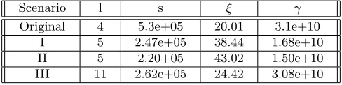
In Figure 2, we fix concrete settings for n, q and γ, thus fixing the desired level of hardness of the cryptosystem. We must then increase l in order to achieve the desired hardness. We record the resulting settings ofl,sandξfor the original R-Dual-Regev encryption scheme and each leakage scenario.
Scenario l s ξ γ
Original 4 5.3e+05 20.01 3.1e+10
I 5 2.47e+05 38.44 1.68e+10
II 5 2.20+05 43.02 1.50e+10
III 11 2.62e+05 24.42 3.08e+10
Fig. 2: The table shows how muchl should be increased to achieve at least the same level of security as the original (no leakage allowed). For each scheme then, the new value for standard deviation of the Gaussian which the secret key (s) and error (ξ) is sampled from is given. For each scenario the obtained approximation factor (γ) is provided. The table is for the case wheren= 1024,q= 4290937559 and`=n/20.
1.3 Our High-Level Approach
For a matrix A = [Ik|A¯] ∈ (Rq) k×l
, where Ik ∈ (Rq) k×k
is the identity matrix and ¯A ∈ (Rq) k×(l−k)
is uniformly random, we define Λ⊥(A) = {z ∈ Rl : Az =0modqR}. By the definition of Aand Λ⊥(A), if, whenx is sampled from some continuous distributionD, we have that [x mod Λ⊥(A)] is uniform random
(over cosets of Λ⊥(A)), then whenxis sampled fromD, the distribution ofAxis also uniform random over
cosets of (qR)k. Both the input distributionDand the output distribution can then be discretized over the ringRto achieve the desired results. Therefore, the goal is to show that whenxis sampled from continuous distributionD, we have that [x mod Λ⊥(A)] is uniform random. Consider the case where the distributionD is exactly a Gaussian distribution with mean 0 and standard deviations. In this case, ifsis greater than or equal to thesmoothing parameter of Λ⊥(A), this by definition ensures that the distribution [x mod Λ⊥(A)] is uniform random. Thus, [28] prove their Regularity Theorem by showing that with high probability over choice ofA, the smoothing parameter,ηε(Λ⊥(A)), is upperbounded bys.
mod Λ] (forn-dimensional lattice Λ) whenxis sampled from a (discrete) Gaussian distribution with mean 0 and sufficiently high standard deviation.
Let ρs :=e−π
hx,xi
s2 and let ψs (the normalization ofρs) correspond to the probability density function
(pdf) of the normalizedn-dimensional Gaussian distribution with mean 0 and standard deviations. To show that the distribution over [x mod Λ] is (close to) uniform whenxis sampled from a distribution with pdf
ψs, one needs to show that for every coset (Λ +c) of the lattice,ψs(Λ +c)≈ 1
det(Λ). Let us focus on showing this for the zero coset, where c = 0 (extending the argument is straightforward due to properties of the Fourier transform). In other words, we would like to show that
X
v∈Λ
ψs(v)≈ 1
det(Λ). (1)
In the following, for a functionf we concisely represent P
v∈Λf(v) byf(Λ).
In order to show (1), we use the Poisson summation formula, which says that for any lattice Λ and integrable functionρs, the following equation holds:
ψs(Λ) = 1
det(Λ)·ψcs(Λ
∨),
where for a functionf,fbdenotes then-dimensional Fourier transform off and Λ∨ is the dual lattice of Λ (see SectionA.2). The task that remains is to show thatψcs(Λ∨) is close to 1 (i.e. is upperbounded by 1 +ε). The general proof approach outlined above can be applied to (integrable) normalized pdfΨ that are not Gaussians centered at 0. Namely, to show that the distribution over [x mod Λ] is (close to) uniform when x is sampled from a distribution with pdf Ψ, one can follow the above template, which implies that it is sufficient to show thatΨb(Λ∨) is upperbounded by 1 +ε.
In this work, we consider pdf’s other than spherical Gaussian distributions centered at 0. In more detail, the pdf,Ψ, we consider corresponds to the probability density function of the secret key, from the point of view of the adversary, given the leakage that is obtained. The technical contribution of this work is then to show that, in each leakage scenario, (with overwhelming probability over choice of ¯A) Ψb(Λ⊥(A)∨) is close to 1. Specifically, for each scenario, our approach requires: (1) Determining the pdfΨ, (2) Computing (an upper bound for) the multi-dimensional Fourier transform ofΨ (denoted Ψb), (3) Proving thatΨb((Λ⊥(A))∨) is upperbounded by 1 +ε(or, equivalently thatΨb((Λ⊥(A))∨\ {0}) is upperbounded byε).
Leakage Scenario I, is fairly simple to handle (given sufficient noise) since if X and Y are multi-dimensional, independent Gaussian random variables, then the distribution of X conditioned on X +Y
is also a multidimensional Gaussian that is not centered at 0. Fortunately, the regularity theorem of [28] straightforwardly extends to Gaussians that are not centered at 0. We mainly view Leakage Scenario I as a warmup to the more difficult Leakage Scenarios II and III.
The analysis for Leakage Scenario II follows from the observation that the distribution ofX conditioned onX+Y is now a non-spherical Gaussian, where leaked coordinates correspond to independent Gaussians with very small standard deviation and unleaked coordinates correspond to independent Gaussians with high standard deviation. The key to analyzing this scenario is noting that the matrix ¯Ais chosen at random, independently of which coordinates are leaked. This allows us to analyze the expectation of Ψb((Λ⊥(A))∨) (correspondingly, the expectation of Ψb((Λ⊥(A))∨\ {0})), over choice of ¯A and show that if not too many coordinates are leaked then the expectation ofΨb((Λ⊥(A))∨\ {0}) remains low. In order for this analysis to go through, the proof of the Regularity Theorem of [28] must be carefully adapted to our setting.
1.4 Summary of Contributions
We next discuss the conceptual and technical contributions of our paper:
– To the best of our knowledge, ours is the first work to analyze the leakage resilience of a Ring LWE-based cryptosystem, with short public keys, that uses power of 2 cyclotomics,Φm, and modulusq≡1 modm. These are the preferred settings for achieving practical efficiency.
– We present a general approach that can be used for obtaining future results on leakage resilience of such schemes. Briefly, our approach involves determining and analyzing the explicit pdf that results from the conditional distribution of the secret key given the leakage (see Section 5). This approach deviates significantly from the approach taken in prior works on leakage resilience. We note, however, that this approach inherently limits the types of leakage functions that can be analyzed.
– As part of the analysis in Scenario II, we re-analyze the regularity theorem from [29] and show the theorem holds for cases where x is drawn from a non-spherical Gaussian with standard deviation significantly
smaller than the smoothing parameter in a constant fraction of the dimensions and standard deviation larger than the smoothing parameter in the remaining dimensions. (See Theorem5.4.) This is a general result that may find further use.
– As part of the analysis in Scenario III, we leverage techniques from the theory of Fourier transforms of radial functions to allow us to take the Fourier transform of a conditional pdf that has a simple representation in spherical coordinates but not in Cartesian coordinates. (See Theorem 5.10.) To the best of our knowledge, these techniques have not been used previously in the lattice-based cryptography literature. We believe that these techniques may have further applications for lattice-based cryptography.
1.5 Related Work
Lattice-based cryptography. Regev introduced the Learning with Errors or LWE, problem in his seminal work [37], and showed aquantum reduction from hardness of solvingLWEproblem to that of solvingGapSVP and SIVP and Peikert [34] showed a classical reduction to GapSVP(but not SIVP). While Regev’s reduc-tion worked for polynomial modulusq, Peikert’s reduction required exponentially large modulus q, and the subsequent work of Brakerski et al. [7] extended the classical reduction to the case of polynomial modu-lus q = poly(n). Regev [37] also presented a public-key encryption scheme based on the hardness of LWE problem. The work of Gentry et al. [19] presented “trapdoor” cryptographic tools from lattices, and also introduced the so-called “Dual-Regev” public key encryption scheme.
Ideal-lattice-based cryptography. Micciancio’s [31] modified Ajtai’s one-way function [1] to the setting of polynomial rings and reduced its security to the hard problem known as thering-SIS problem. Lyubashevsky et al. [27] introduced thering-LWEproblem and proved its hardness by proving aquantum reduction toSVP on arbitrary ideal lattices arising from the ringR. In an independent work, Stehl´e et al. [39] also considered a special case of ring-LWE and proved the hardness for only search problem for the specific ring. Ring-LWE problem can be used to construct public key encryption [27,28,29]. In particular, Lyubashevsky et al. [28,29] presented the analogue of the “Dual-Regev” public key encryption scheme for the ring-LWE setting.
Leakage-resilient cryptography. There is a significant body of work on leakage-resilient cryptographic primi-tives, beginning with the work of Dziembowski and Pietrzak [17] on leakage-resilient stream-ciphers. Other constructions include [35,2,33,6,26,23,23,5,30,14,26] With the exception of [2], most of these results construct new cryptosystems from the bottom up. In our work, we consider whether we can prove that an existing cryptosystem enjoys leakage resilience, without modification of the scheme.
onLWEwhich is secure against an adversary learning any computationally uninvertible function of the secret key.
2
Notation and Preliminaries
For a positive integern, we denote by [n] the set{1, . . . , n}. We denote vectors in boldface xand matrices
using capital letters A. For vector xover Rn or
Cn, define the `2 norm as kxk2 = ( P
i|xi| 2
)1/2. We write as kxk for simplicity. We present the background and standard definitions related to lattices and algebraic number theory in SectionAof Supporting Material. We next present the formal definition of the ring-LWE problem as given in [29].
Definition 2.1(Ring-LWE Distribution). For a “secret”s∈R∨
q (or justR∨) and a distributionψover
KR, a sample from the ring-LWE distribution As,ψ overRq×(KR/qR
∨) is generated by choosing a ←R
q
uniformly at random, choosinge←ψ, and outputting(a, b = a·s+emodqR∨).
Definition 2.2 (Ring-LWE, Average-Case Decision). The average-case decision version of the
ring-LWEproblem, denoted R-DLWEq,ψ, is to distinguish with non-negligible advantage between independent
sam-ples from As,ψ, where s←R∨q is uniformly random, and the same number of uniformly random and
inde-pendent samples fromRq×(KR/qR
∨).
In [3], it is shown that an equivalent “tweaked” form of the Ring-LWE problem can be used in cryp-tographic applications without loss in security or efficiency. This is convenient since the “tweaked” version does not involveR∨. The “tweaked” ring-LWE problem can be obtained by implicitly multiplying the noisy products bi by the “tweak” factor t = ˆm/g ∈ R as defined in definition A.2. Note that, t·R∨ =R. This yields new values
bi0 = t·bi = (t·s)·ai+ (t·ei) = s0·ai+ei0modqR,
where ai, s0 =t·s∈Rq, and the errors ei0 =t·ei come from the “tweaked” error distribution t·ψ. Note that whenψ corresponds to spherical Gaussian, its tweaked formt·ψ may behighly non-spherical.
Theorem 2.3. [29, Theorem 2.22] LetK be the mth cyclotomic number field having dimension n=ϕ(m)
and R = OK be its ring of integers. Let α = α(n) > 0, and q = q(n) ≥ 2, q = 1 modm be a poly(n)
-bounded prime such thatαq≥ω(√logn). Then there is a polynomial-time quantum reduction fromO˜(√n/α) -approximateSIVP(orSVP) on ideal lattices inKto the problem of solving R-DLWEq,ψ given only lsamples,
whereψ is the Gaussian distributionDξ forξ=α·q·(nl/log (nl)) 1/4
.
2.1 Security Definitions for Leakage Resilient Public Key Encryption
A public key encryption schemeE consists of three algorithms: (Gen,Enc,Dec).
– Gen(1n)→(pk,sk). TheGen takes in the security parameter and outputs a public keypk and a secret keysk.
– Enc(pk, m)→c. TheEnctakes in a public keypkand a messagem. It outputs a ciphertextc. – Dec(sk, c)→m. TheDec takes in a ciphertextcand a secret keysk. It outputs a messagem.
Correctness. The PKE scheme satisfies correctness if Dec(sk, c) = m with all but negligible probability wheneverpk,skis produced byGen andcis produced byEnc(pk, m).
Security. We define IND-CPA security under non-adaptive, one-time leakage for PKE schemes in terms of the following game between a challenger and an attacker (this extends the usual notion of IND-CPA security to our leakage setting). We letndenote the security parameter, and the classF denotes the class of allowed leakage functions.
Setup Phase. The game begins with a setup phase. The challenger calls Gen(1n) to create the initial secret keyskand public keypk.
Challenge Phase. The attacker receives (pk, f(sk)) from the challenger. The attacker chooses two messages
m0,m1which it gives to the challenger. The challenger chooses a random bitb∈ {0,1}, encryptsmb, and gives the resulting ciphertext to the attacker. The attacker then outputs a guess b0 for b. The attacker
wins the game ifb=b0. We define the advantage of the attacker in this game as 1 2 −Pr[b
0=b] .
Definition 2.4(IND-CPA security under Non-Adaptive, One-Time Leakage). We say a Public Key Encryp-tion schemeE= (Gen,Enc,Dec)is IND-CPA secure under non-adaptive, one-time key leakage from leakage classF if any probabilistic polynomial time attacker only has a negligible advantage (negligible inn) in the above game.
3
Regularity and Fourier Transforms
Letρs,c denote an n-dimensional Gaussian function with standard deviationsand meanc.
One and Multi-Dimensional Gaussians. Fors >0,c∈R,x∈R, define the Gaussian functionρ1s,c:R→(0,1] as
ρ1s,c(x) :=e−π(sx2−c)2.
Whenc= 0, we write for simplicity,
ρ1s(x) :=e−πs(2x)2.
By normalizing this function we obtain the continuous Gaussian probability distributionψ1
s,c (resp.ψ1s) of parameters, whose density is given bys−1·ρ1
s,c(x) (resp. s−1·ρ1s(x)). We denote byρ(s1,...,sn),(c1,...,cn) the distribution overR
n with the following pdf:
Letρ1s,cdenote a one-dimensional Gaussian function as above with standard deviationsand meanc.We denote byρ(s1,...,sn),(c1,...,cn)the distribution over R
n with the following pdf:
ρ(s1,...,sn),(c1,...,cn)(x1, . . . , xn) :=ρ
1
s1,c1(x1)· · ·ρ 1
sn,cn(xn).
When c = 0, we again write for simplicity, ρ(s1,...,sn). Moreover, when s1 = · · · = sn and the dimension
is clear from context we write for simplicity ρs,(c1,...,cn) (resp. ρs). Normalizing as above, we obtain the
correspondingcontinuous Gaussian probability distributionψ(s1,...,sn),(c1,...,cn)(resp.ψ(s1,...,sn),ψs,(c1,...,cn), ψs).
Definition 3.1(Fourier Transform). Given an integrable functionf :Rn→C, we denote by fb:Rn→C
the Fourier transform of f, defined as
b
f(y) := Z
Rn
f(x)e−2πihx,yidx.
Theorem 3.2 (Poisson Summation Formula). Let f : Rn → C be a nice enough function9 and Λ a
lattice of dimension n. Then
f(Λ) = 1 det(Λ)fb(Λ
∨),
whereΛ∨ is the dual lattice ofΛ and
b
f is a Fourier transform off.
Definition 3.3. For ann-dimensional lattice Λ, and positive realε >0, we define its smoothing parameter ηε(Λ)to be the smallest ssuch that ρ1/s(Λ∨\ {0})≤ε.
Lemma 3.4. [32,10] For anyn-dimensional latticeΛ, we have
√ ln(1/ε)
√
πλ1(Λ∨) ≤ηε(Λ)≤
√
n
λ1(Λ∨), forε∈[2
−n,1].
9
Assume thatR
Claim ( [29]).For anyn-dimensional lattice Λ and ε, s >0,
ρ1/s(Λ)≤max
1,
ηε(Λ∨)
s
n
(1 +ε).
Lemma 3.5. For anyn-dimensional latticeΛandε >0,s:= (s1, . . . , sn)∈Rn>0, andc:= (c1, . . . , cn)∈Rn,
if all ofs1, . . . , sn < ηε(Λ∨)then
ρ(1/s1,...,1/sn),(c1,...,cn)(Λ)≤
ηε(Λ∨)
s1
· · ·ηε(Λ
∨)
sn
(1 +ε).
The proof can be found in Section Bin supplementary material.
Lemma 3.6. [32, Lemma 3.6] For any latticeΛ, positive reals >0 and a vectorc,ρs,c(Λ)≤ρs(Λ).
Definition 3.7. Let Λ be an n-dimensional lattice and Ψ a probability distribution over Rn. Define the
discrete probability distribution ofΨ overΛto be:
DΛ,Ψ(x) =
Ψ(x)
Ψ(Λ),∀x∈Λ.
Definition 3.8. LetΛbe ann-dimensional lattice, define the discrete Gaussian probability distribution over
Λ with parameter(s1, . . . , sn)and center(c1, . . . , cn)as
DΛ,(s1,...,sn),(c1,...,cn)(x) =
ρ(s1,...,sn),(c1,...,cn)(x) ρ(s1,...,sn),(c1,...,cn)(Λ)
,∀x∈Λ.
Remark 1. WheneverΨis Gaussian with parameter (s1, . . . , sn) and center (c1, . . . , cn) we denote it’s discrete Gaussian probability by DΛ,(s1,···,sn),(c1,...,cn). If s = s1 = · · · = sn (resp. c = c1 = · · · = cn) we write DΛ,s,(c1,...,cn)(resp.DΛ,(s1,...,sn),c). Ifc1=· · ·=cn= 0 we writeDΛ,(s1,···,sn).
Lemma 3.9. [32, Lemma 4.4] For anyn0-dimensional latticeΛ, and reals0< ε <1, s≥η
ε(Λ), we have
Pr
x∼DΛ,ψs
kxk> s√n0≤ 1 +ε
1−ε ·2
−n0.
The following is a modified version of Lemma 3.8 from [37] and the proof can be found in Section Bin supplementary material.
Lemma 3.10. LetΛbe ann-dimensional lattice andΨ a probability distribution overRn. If|Ψb|(Λ∨\ {0})≤
ε, then for anyc∈Rn,Ψ(Λ +c)∈det(Λ∨)(1±ε), where|Ψb|(Λ∨\{0})denotes the summation of the absolute
value of the function at each point inΛ∨\ {0}.
The proof of the following lemma proceeds as the proof of Corollary 2.8 in [19].
Lemma 3.11. LetΛ0 be ann-dimensional lattice andΨ a probability distribution overRn. Assume that for
allc∈Rn it is the case that
Ψ(Λ0+c)∈ 1−ε
1 +ε,
1 +ε
1−ε
·Ψ(Λ0),
LetΛbe ann-dimensional lattice such thatΛ0 ⊆Λthen the distribution of(DΛ,Ψ mod Λ0)is within statistical
distance of at most4εof uniform over (Λ mod Λ0).
Definition 3.12. For a matrixA∈Rk×l
q we defineΛ⊥(A) = {z∈Rl :Az= 0 modqR},which we identify
Theorem 3.13. [29] LetR be the ring of integers in the mthcyclotomic number field K of degreen, and q≥2 an integer. For positive integersk≤l≤poly(n), letA = [Ik|A¯]∈(Rq)
k×l
, where Ik ∈(Rq) k×k
is the identity matrix and A¯∈(Rq)
k×(l−k)
is uniformly random. Then for alls≥2n,
EA¯ρ1/s Λ⊥(A)
∨
≤ 1 + 2(s/n)−nlqkn+2+ 2−Ω(n).
In particular, ifs >2n·qk/l+2/(nl) then EA¯
ρ1/s Λ⊥(A)∨
≤ 1 + 2−Ω(n), and so by Markov’s inequality, η2−Ω(n)(Λ⊥(A))≤sexcept with probability at most 2−Ω(n).
The following corollary was presented in [29].
Corollary 3.14. LetR, n, q, k andlbe as in Theorem3.13. Assume thatA = [Ik|A¯]∈(Rq)k×l is chosen as
in Theorem3.13. Then, with probability1−2−Ω(n) over the choice ofA, the distribution of¯ Ax∈Rk q, where
each coordinate of x∈Rl
q is chosen from a discrete Gaussian distribution of parameter s >2n·qk/l+2/(nl)
overR, satisfies that the probability of each of theqnk possible outcomes is in the interval (1±2−Ω(n))q−nk
(and in particular is within statistical distance 2−Ω(n) of the uniform distribution over Rk q).
We next state an additional corollary of the regularity theorem from [29].
Corollary 3.15. Let R, n, q, k andl be as in Theorem3.13. Assume that A = [Ik|A¯]∈(Rq) k×l
is chosen as in Theorem 3.13. Then, with probability1−2−Ω(n) over the choice ofA, the shortest non-zero vector in¯ Λ⊥(A)∨ has length at least
√ n/π 2n·qk/l+2/(nl).
The following lemma computes a lower bound of the normalization factor of the pdf in Theorem 3.17. The proof can be found in SectionBof supplementary material.
Lemma 3.16. Let n0 ∈Nbe odd, x∈Rn
0
,c∈R. Then
Z
Rn0e
−π(kxk−c)2
σ2 +e−
π(kxk+c)2
σ2 dx≥σn0.
The next theorem provides an upper bound on the Fourier transform of a pdf for the subsequent analysis of Leakage Scenario III in Section5.3. We refer to SectionB.1of Supporting Material for the detailed proof.
Theorem 3.17. Letn0:=l·2a+ 1, wherel, a are positive integers anda >2, andc≤σ·√2·√n0. LetΨ
σ,c
denote the normalized pdf corresponding to the non-normalized function f(x) :=e−π(kxk−σ2c)2 +e−
π(kxk+c)2
σ2 ,
wherexis a vector overn0 dimensions. and letΨdσ,c(y)denote then0-dimensional Fourier transform ofΨσ,c.
Then|Ψdσ,c(y)| ≤n0 n0
·e−πkyk2σ2 forkyk>1/σ.
4
Dual-Style Encryption Scheme
In this section we present a dual-style encryption scheme from [29], with “tweaking” introduced by [3,11]. The system is parameterized by l, which is the number of R-LWE samples which attacker gets to see;q is the modulus of the ringRq; s, ξ are the parameters for the continuous Gaussian distributions ψs, and ψξ over cyclotomic field KR respectively. Also, let DR,s be the discrete Gaussian distribution obtained from
ψs, where R denotes mth cyclotomic ring (of degree n =ϕ(m)). Also, let p, q be coprime integers.10 Let b·e be a valid discretization. Then the corresponding “tweaked” distribution over R or pR is defined as
ψpR = bt·p·ψ
ξepR. Similarly, ψµ+pR = bt·p·ψξeµ+pR. 11 The dual-style encryption scheme consists of three algorithm as follows:
Key-Generation Algorithm Gen: It outputs private/public key pair by following steps.
10
In this work we consider p = 2, while computing the parameters presented in tables 1 and 2. Note that, the encryption scheme and analysis holds for any generalpcoprime withq.
1. Choosea1=−1∈Rq, and generate uniformly random and independent elementa2, . . . , al∈Rq. 2. Generate independentx1, . . . , xl←DR,s.
3. Set the public keya= (a2, . . . , al, al+1=−Pi∈[l]aixi)∈Rlq, and the secret keyx= (x2, . . . , xl, xl+1= 1)∈Rlq. Note thatha,xi=x1∈Rq by construction.
Encryption Algorithm Enc: It takes as input a public key a ∈ Rl
q, and a message µ ∈ Rp, returns a ciphertextcby proceeding the following steps.
1. Generate independente1, . . . , el←ψpR andel+1←ψµ+pR. Sete= (e2, . . . el+1)∈Rl.
2. Computec=e1·a+e∈Rlq.
Decryption Algorithm Dec: It takes as input a private key x∈Rlq, and a ciphertext c∈ Rlq, returns a plaintextµby proceeding the following steps.
1. Computed=hc,xi ∈R. 2. Output µ=dmodpR.
Lemma 4.1. Let the view of the adversary be viewA= (a,leak), where leak is the leakage obtained by the
adversary as defined in section2.1. If the public key elemental+1 is close to uniform givenviewA, then the
above encryption scheme is IND-CPA secure assuming the hardness of R-DLWEq,ψξ givenl+ 1 samples.
Proof of lemma 4.1 and correctness can be shown as in [29]. We present the details in Section C of Supporting Material.
5
Security against Auxiliary Inputs
In this section and SectionDof Supporting Material, we analyze security against auxiliary inputs under three scenarios. For each leakage scenario, we argue that the encryption scheme defined in Section4still achieves semantic security. To prove this, it is sufficient to show, in each scenario, thatconditioned on the view of the leakage adversary, the distribution overAxremains (close to)uniform random. In other words, we show that the distribution over Ax remainsuniform random, even when x is drawn from a conditional distribution corresponding to the knowledge the adversary has aboutx, conditioned on the leakage that was obtained. This informal statement is made formal in Corollaries5.3,5.8and5.11for each of the leakage scenarios I, II and III. Details of leakage analysis on scenarios I can be found in SectionDof Supporting Material. In this section, we only focus on analyzing security against leakage scenarios II and III.
5.1 Leakage Scenario I
Recall that the secret key of the encryption scheme defined in Section4 is (x1, . . . , xl), where each xi ∈Rq is chosen from a discrete Gaussian distribution DR,s, where s > 2n·qk/l+2/(nl). In this scenario we can assume that eachxiis stored using the polynomial representation (powerful basis) and allow leakage oneach coefficient or assume that each xi is stored using the canonical embedding (CRT basis) and allow leakage oneach coordinate (this is because for power-of-two cyclotomics, spherical Gaussians in the powerful basis representation correspond to spherical Gaussians in the CRT basis representation). We assume, however, that the leakage is “noisy” in the sense that independent Gaussian noise (with sufficiently high standard deviation) is added to each leaked coordinate. More precisely, adversary learns a “noisy” version of secret key, where independent Gaussian noise with standard deviationv is added to each coordinate of the secret key.
It turns out that this scenario is actually quite simple to handle (given sufficient noise) since if X and
Y are independent Gaussian random variables, then the distribution ofX conditioned on X+Y is also a Gaussian that isnot centered at 0. Fortunately, the regularity theorem of [29] straightforwardly extends to Gaussians that are not centered at 0.
We discuss formal details next, however, we mainly view Leakage Scenario I as a warm-up to the more difficult Leakage Scenarios II and III discussed below.
X at valuex, sampled from n-dimensional Gaussian distribution with each component of variable pairwise independent, as
GX(x,u,s) = Y
i∈[n] 1
si exp
−π(x i−ui)2
s2 i
,
with mean u = (u1, . . . , un) and standard deviation s = (s1, . . . , sn). The probability density function of
Y at value y, sampled from n-dimensional Gaussian distribution with each component of variable pairwise independent, can be written as
GY(y,µ,v) = Y
i∈[n] 1
vi exp
−π(y i−µi)2
v2 i
,
with meanµ= (µ1, . . . , µn) and standard deviation v= (v1, . . . , vn).
We now consider the distribution of the secret key X, conditioned on the leakage X +Y. We proceed with the following straightforward lemma:
Lemma 5.1. Given two independent random variables X and Y. Suppose that the distribution of X is a n-dimensional Gaussian distribution with meanu and standard deviation s, each component ofX pairwise independent, and the distribution ofY is a n-dimensional Gaussian distribution with meanµand standard deviationv, each component ofY pairwise independent. Then the distribution ofX conditioned onX+Y =z is also a n-dimensional Gaussian distribution, where each component ofX is pairwise-independent with mean
c:= (c1, . . . , cn)whereci:=
ui s2i−
µi vi2+
zi v2i
1
s2i+
1
vi2
and standard deviationσ:= (σ1, . . . , σn), whereσi := r
1 1
s2i+
1
v2i .
The proof can be found in Appendix D.
Let v := (v, . . . , v) and s := (s, . . . , s) and let v = τ ·s. Suppose the distribution of secret key is
GX(x,0,s) and the distribution of noise is GY(y,0,v), on the condition that adversary learns some fixed leakagez(corresponding to the ”noisy” secret key), Lemma5.1shows that the distribution of secret key, in the view of adversary who has obtainedz, is
Y
i∈[n×l] 1
σexp
−πxi−τ2z+1i 2
σ2
Thus, from the viewpoint of the adversary, each coordinatexiof the secret key is sampled from a multivariate
Gaussian distribution ρσ,ci with mean ci := (ci1, . . . , cin), where cij :=
zj
τ2+1 and σ = s q
τ2
τ2+1. The entire secret key is then sampled fromρσ,c, wherec= [ci]i∈l.
We have the following theorem:
Theorem 5.2. LetRbe the ring of integers in themthcyclotomic number fieldK of degreen, andq≥2an
integer. For positive integers k≤l≤poly(n), let A = [Ik|A¯]∈(Rq)k×l, where Ik ∈(Rq)k×k is the identity
matrix andA¯∈(Rq)k×(l−k) is uniformly random. Then for all σ≥2n·qk/l+2/(nl) andc∈
Rn·l then
d
ρσ,c Λ⊥(A)∨ ≤ 1 + 2−Ω(n),
except with probability at most2−Ω(n) over choice ofA.¯
Proof. It follows from Lemma3.6and regularity theorem from [29].
The following corollary follows from Lemmas 3.10and3.11and Theorem5.2.
Corollary 5.3. Let R, n, q, k, l,c, σ be as in Theorem5.2. Assume that A = [Ik|A¯]∈(Rq) k×l
is chosen as in Theorem5.2. Then, with probability1−2−Ω(n) over the choice of A, the distribution of¯ Ax∈Rkq, where x∈Rl is chosen fromD
Λ,σ,c, the discrete Gaussian probability distribution overRl with parameterσ and
centerc, satisfies that the probability of each of theqnkpossible outcomes is in the interval (1±2−Ω(n))q−nk
(and in particular is within statistical distance 2−Ω(n) of the uniform distribution over Rk q).
The above corollary implies that the encryption scheme is secure under Leakage Scenario I assuming
σ ≥ 2n·qk/l+2/(nl). Since s = q1+τ2
τ2 ·σ, it means that in order for the encryption scheme to be secure under Leakage Scenario I, we must simply sample the secret key from D
Rl,q1+τ2
τ2 ·2n·q
k/l+2/(nl), as opposed toDRl,2n·qk/l+2/(nl). In particular, this means that the standard deviation should be increased by a factor of q
1+τ2
τ2 , beyond the parameters required by [29].
5.2 Leakage Scenario II
Recall that in this scenario we leak a constant fraction of the coordinates ((`·l)/(l·n)-fraction) with low noise added to each leaked coordinate (only 2nstandard deviation, as opposed to√2·2n·qk/l+2/(nl)standard deviation as in Leakage Scenario I, whenv=s). Recall that the secret key of the encryption scheme defined in Section4 is (x1, . . . , xl), where each xi ∈Rq. We assume that eachxi will be stored as a vector in the canonical embedding (CRT basis).
Thus, this scenario allows leakage of`out ofxi fori∈[l] with restriction that the coordinates leaked for eachxiis same across all differentxis. Since conditioned on the leakage, the distribution over the secret key is no longer a spherical Gaussian, we can no longer switch between the powerful and CRT basis as before.12 The analysis for this leakage scenario follows from a careful adaptation of the proof of the Regularity Theorem of [29] to our setting.
Suppose the distribution of secret key is GX(x,0,s) where s = {s, s, ..., s}. The adversary learns the leaked “noisy” secret keyz in`positions, where the noise is sampled from Gaussian distribution with mean = 0 and standard deviation≈2n. LetS ⊆[n], where|S|=`denote the set of positions (from eachxi) that are leaked. Lemma5.1shows that, conditioned on leakage, each componentxji,i∈[l], j∈ S, of secret key is
sampled from Gaussian distribution with meancji := nz
j i
n+1
s2
, and varianceσj2≥4n2. Conditioned on leakage,
each componentxji,i∈[l], j /∈ S, of the secret key is sampled from Gaussian distribution with meancji = 0, and varianceσ2
j =s2.
Theorem 5.4. Let R be the ring of integers in the mth cyclotomic number field K of degree n, where n
is a power of 2, q is a prime satisfying q = 1 modm. For positive integers k ≤ l ≤ poly(n), let A = [Ik|A¯]∈(Rq)
k×l
, where Ik ∈(Rq) k×k
is the identity matrix and A¯∈(Rq)k×(l−k) is uniformly random. Let
σ := (σ1, . . . , σn)∈Rn>0 andc:= (c1, . . . , cln)∈Rln be vectors, where σ is such that `positions are set to 2n, while the other positions are set to s. Letk, l, `be such thatl−k−l·`/n >0 andl−k−1≥1, and let
s≥2n·qlkn(n−+2`) then d
ρσl,c Λ⊥(A)∨ ≤ 1 + 2−Ω(n)except with probability at most 2−Ω(n) over choice of A.¯
For proving Theorem 5.4, we begin with exposition on the forms of the Ideals qR∨ ⊆ J ⊆ R∨ in power-of-two cyclotomics as well as some lemmas. These will then be useful in the proof of Theorem5.4.
To generate the setTof idealsJ such thatqR∨⊆ J ⊆R∨we can take each idealIsuch thatqR⊆ I ⊆R
and setJ :=qI∨.
Recall from Fact A.3 that hqi splits completely into n distinct ideals of norm q, i.e. qR = Πi∈[n]pi. Therefore, the set of all ideals I such that qR⊆ I ⊆R, is exactly the setS :={Πi∈Spi | S ⊆[n]}. Thus,
12
the number of ideals I such thatqR⊆ I ⊆R (and hence also the number of ideals J ∈T) is exactly 2n. Moreover, note that for each idealJ ∈T,
|J/qR∨|=|R/qJ∨|=N(qJ∨).
Thus, we see that for eachJ ∈T,1≤ |J/qR∨| ≤qn.
LetT1 denote the set of idealsJ ∈T such that|J/qR∨|<2n.
LetT2 denote the set of idealsJ such that|J/qR∨| ≥2n. Furthermore, letT21be the set ofJ ∈T2such thats≥η2−2n((1qJ)∨). LetT22:=T2\T21.
Letσ := (σ1, . . . , σn)∈Rn>0 be a vector with` positions are set to 2n, while the other positions are set to values.
Lemma 5.5. For idealsJ ∈T1,
η2−2n
(J
q)
∨≤2n.
Proof.
η2−2n
(J
q)
∨≤
√
n
λ1
(Jq)∨
(2)
≤
N
J
q
−1/n
(3)
≤(|J/qR∨| ·nn)1/n (4)
≤(2n·nn)1/n (5)
= 2n,
where (2) follows from Lemma 3.4, (3) follows from Lemma A.1, and (4) follows from the fact that
NJq
−1
=|J/qR| =|R∨/R| · |J/qR∨| =∆K|J/qR| (for example, see [9, page. 63]), and (5) follows from the definition ofT1.
Lemma 5.6. For idealsJ ∈T1 2
|J/qR∨|−(l−k) ρ
1/σ1,...,1/σn
1
qJ
l!
≤2−n(l−k)
Proof. Recall thatσ:= (σ1, . . . , σn)∈Rn>0 is defined as a vector such that `positions are set to 2n, while the other positions are set tos. Define z1, . . . , zn in the following way: For i ∈[n], ifσi =s thenzi =σi.
Otherwise,zi=η2−2n
(1qJ)∨. Applying Poisson summation twice we arrive at:
ρ1/σ1,...,1/σn
1
qJ
= 1/det(1
qJ)·(1/σ1· · ·1/σn)ρσ1,...,σn
(1
qJ)
∨
(6)
≤1/det(1
qJ)·(1/σ1· · ·1/σn)ρz1,...,zn
(1
qJ)
∨
(7)
= η2
−2n((1
qJ)
∨)
2n
!`
·ρ1/z1,...,1/zn
1
qJ
(8)
≤(1 + 2−2n)· η2
−2n((1qJ)∨)
2n
!`
, (9)
Lemma 5.7. For any lattice L∨,
ρs1,...,sn(L) =s1·s2·. . .·sn·
1
det(L)·ρ1/s1,...,1/sn(L
∨)
Proof. It can be easily verified by combining Poisson Summation formula and the fact that ˆρs1,...,sn = s1· · ·snρ1/s1,...,1/sn.
By replacing si with 1/zi for alliand replacingL with 1qJ, we have
1/det(1
qJ)·ρz1,...,zn
(1
qJ)
∨
=z1· · ·zn·ρ1/z1,...,1/zn
1
qJ
.
By plugging into (7), we have
z1
σ1 · · · zn
σn
·ρ1/z1,...,1/zn
1
qJ
By definition ofzi, zi
σi = 1 when σi=sand
zi
σi =
η2−2n((1qJ)
∨)
2n , whenσi= 2n. Since there are` positions in σ whenσi= 2n, we obtain (8). Finally (9) follows by definition of smoothing parameterη2−2n((1
qJ)
∨).
Now, using the fact thatη2−2n≤(∆K|J/qR∨|)1/n, the fact that ∆K =nn and the fact that|J/qR∨| ≥
2n, and the set of parameters, we have that
|J/qR∨|−(l−k) ρ
1/σ1,...,1/σn
1
qJ
l!
≤ |J/qR∨|−(l−k−l·`/n)(1 + 2−2n)l·2−`·l
≤2−n(l−k)
which completes the proof of the lemma.
We now conclude the proof of Theorem 5.4.
Proof of Theorem 5.4. Since by Lemma3.6 we have that for any (n·l)-dimensional vectors, c,x and any
n-dimensional vectorσ= (σ1, . . . , σn):
d
ρσl,c(x)≤
c
ρσl(x) =ρ(1/σ
1,...,1/σn)l(x),
then following the proof of [29] step-by-step, it is sufficient to show that
X
J ∈T
|J/qR∨|−(l−k)· ρ(1/σ1,...,1/σn)
1
qJ
l −1
!
≤2−Ω(n).
We will show that
X
J ∈T2 1
|J/qR∨|−(l−k) ρ
(1/σ1,...,1/σn)
1
qJ
l −1
!
≤2−Ω(n), (10)
and that
X
J ∈(T1∪T22)
|J/qR∨|−(l−k) ρ
1/σ1,...,1/σn
1
qJ
l −1
!
≤2−Ω(n) (11)
To show (11), note that by Lemma5.5, for idealsJ ∈T1 (we have thatη2−2n((Jq)∨)≤2n. This means
that for eachi∈[n], σi≥η2−2n, which implies thatρ1/σ1,...,1/σn
1 qJ
l
On the other hand, by definition of T22, for ideals J ∈ T22, we have that σi < η2−2n, for each
i∈[n]. Thus, by Lemma3.5 we have thatρ1/σ1,...,1/σn
1 qJ
≤
η2−2n((Jq)∨)
σ1 · · ·
η2−2n((Jq)∨)
σn
·(1 + 2−2n).
Since η2−2n((Jq)∨)n ≤ |J/qR∨|∆K, and plugging in the proper values for σ1, . . . , σn, we have that
ρ1/σ1,...,1/σn
1 qJ
l
≤ (|J/qR∨|∆Ks−n+`·(2n)−`)l·(1 + 2−2n)l. Combining the above, we get that for J ∈T1∪T22,
ρ1/σ1,...,1/σn
1
qJ
l
≤max(1,(|J/qR∨|∆Ks−n+`·(2n)−`)l)·(1 + 2−2n)l.
Thus, similarly to [29], using the lower bound ofsfrom the setting, we can bound
X
J ∈(T1∪T2 2)
|J/qR∨|−(l−k) ρ
1/σ1,...,1/σn
1
qJ
l −1
!
≤ X
J ∈(T1∪T22)
|J/qR∨|−(l−k)·max(1,(|J/qR∨|∆
Ks−n+`·(2n)−`)l)·(1 +ε)l
≤ X
J ∈T
|J/qR∨|−(l−k)·max(1,(|J/qR∨|∆Ks−n+`·(2n)−`)l)·(1 +ε)l
≤2−Ω(n)+ 2(s/n)−nlqkn+2 s
2n
l·`
∈2−Ω(n).
Moreover, by Lemma5.6and the fact that|T21| ≤ |T|= 2n, we can bound
X
J ∈T1 2
|J/qR∨|−(l−k) ρ
1/σ1,...,1/σn
1
qJ
l −1
!
≤2n·2−n(l−k)∈2−Ω(n),
where the last line follows from the setting of parameters. This completes the proof.
The following corollary follows from Lemmas 3.10and3.11and Theorem5.4.
Corollary 5.8. LetR, n, q, k, l, `,σandcbe as in Theorem5.4. Assume thatA = [Ik|A¯]∈(Rq) k×l
is chosen as in Theorem5.4. Then, with probability1−2−Ω(n)over the choice ofA, the distribution of¯ Ax∈Rk
q, where x∈Rlis chosen fromD
Rl,σl,c, the discrete Gaussian probability distribution overRl with parameterσland
centerc, satisfies that the probability of each of theqnkpossible outcomes is in the interval (1±2−Ω(n))q−nk
(and in particular is within statistical distance 2−Ω(n) of the uniform distribution over Rk q).
Specifically, the above corollary implies that the encryption scheme is secure under Leakage Scenario II
assumings≥2n·qlkn(n−+2`) Sinceσ:=s, whereσ is the standard deviation of the secret key, it means that in order for the encryption scheme to be secure under Leakage Scenario II, we must simply sample the secret key fromD
R,2n·q
kn+2
l(n−`), as opposed toDR,2n·q
k/l+2/(nl). In particular, this means that the standard deviation
should be increased from 2n·qk/l+2/(nl) (as in [29]) to 2n·qlkn(n−+2`).
5.3 Leakage Scenario III
We slightly change the encryption scheme from Section 4 so that the secret key is represented by a vector of dimension n0 := l·n+ 1, wheren is a power of two. Note that when n is a power of two, a spherical Gaussian in the coefficient representation is also a spherical Gaussian in the canonical embedding repre-sentation [27]. Thus, we can assume that the secret key is generated using the coefficient representation, where each coordinate is sampled independently from a discrete Gaussian, DZ,s0. During key sampling, an
In this scenario, the adversary learns the magnitude of the secret key with channel error, where both secret key and error are sampled from Gaussian distributions. Our key observation for the analysis of Leakage Scenario III is that the probability of a particular secret key vector x under the conditional distribution corresponding to the view of the adversary stilldepends only on the magnitude ofx. This allows us to show that the probability density function (PDF) corresponding to the conditional distribution overx, conditioned on the leakage has the form of a one-dimensional Gaussian, when viewing the pdf as aradial function over a single variable r = kxk. Using properties of radial Fourier transforms, we are then able to analyze this setting.
Recall that a generic PDF of one dimensional Gaussian distribution is defined as:
G(x, u, s) =1
sexp
−π(x−u)2
s2
,
where uis mean, and s is standard deviation of the distribution. We write probability density function of secret keyX at valuex= (x1, . . . , xn0), of which each coordinate is independently sampled from a Gaussian
distribution with center at 0 and standard deviations, as
GX(x, s) = Y i∈[n0]
1
sexp
−πx2
i
s2
= 1
sn0 exp
−πr2
s2
=GR(r, s),
whereris the magnitude ofx. It also can be viewed as probability density function of secret key magnitude
R, denoted as GR(r, s). The error is sampled from a 1-dimensional Gaussian distribution with center at 0. We write probability density function of errorE at valuey is
GE(y, v) =1
vexp
−πy2
v2
.
Let FZ|A(Z = b) generically represent the probability density function of random variable Z at value b,
conditioned on eventA. We can then derive the density function of secret key magnitudeR given the value
z of|R+E|. In other words, the weight placed on a valuex= (x1, . . . , xn0) by the conditional distribution
dependsonly on the magnitude of x(i.e.r=kxk) and can be computed as:
F
R|R+E|=z
(R=r) =FR,R+E(R=r,|R+E|=z)
FR+E(|R+E|=z)
=GR(r, s)GE(z−r, v) +GR(r, s)GE(−z−r, v)
FR+E(R+E=z) +FR+E(R+E=−z)
=R GR(r, s)GE(z−r, v) +GR(r, s)GE(−z−r, v)
Rn0GR(|x|, s)GE(z− |x|, v) dx+RRn0GR(|x|, s)GE(−z− |x|, v) dx
=e
−(π s2+vπ2)
r− zs2
v2 +s2 2
+e−(sπ2+vπ2)
r+ zs2 v2 +s2
2
nVnR
∞ −∞e
−(π s2+vπ2)
r− zs2
v2 +s2 2
rn−1dr
=e
−(π s2+vπ2)
r− zs2
v2 +s2 2
+e−(sπ2+vπ2)
r+ zs2 v2 +s2
2
N , (12)
whereN is the normalization factor.
It is easy to see that the probability density function F
R|R+E|=z
(R =r) is the sum of two Gaussian
probability density functions center at v2zs+2s2 and − zs2
v2+s2 respectively with the same standard deviationσ. Supposev=s, we haveσ= √s
2.
Lemma 5.9. Supposev=s, we can bound a centerv2zs+2s2 from Equation12byPr
zs2 v2+s2 ≥s
√
Proof of Lemma 5.9. Using union bound, we have
Pr zs2
v2+s2 ≥s √
n0
= Prz 2 ≥s
√
n0
≤PrR+E≥2s√n0+ Pr−R−E≥2s√n0
≤PrR≥s·√n0+ PrE≥v√n0+ PrE≥v√n0
By Lemma3.9and LemmaD.1, we deduce that Prv2zs+2s2 ≥s √
n0∈2−Ω(n).
Recall that conditioned on the leakage, the weight placed by the conditional distribution on a vector x∈Rn
0
is equivalent toF
R|R+E|=z
(R =r), where r=kxk. LetΨσ,c(x) :=FR |R+E|=z
(R =kxk) be the
normalization of the functionf(x) :=e−π(
kxk−c)2
σ2 +e−
π(kxk+c)2
σ2 . As shown in Lemma5.9above, we have that with all but negligible probability,c:=v2zs+2s2 ≤
√
2·σ√n0. We next present the following Theorem.
Theorem 5.10. LetR be the ring of integers in themth cyclotomic number fieldK of degree n, wherenis
a power of two. For positive integers k≤l ≤poly(n), letA = [Ik|A¯]∈(Rq) k×l
, whereIk∈(Rq) k×k
is the
identity matrix andA¯ ∈(Rq) k×(l−k)
is uniformly random. Letc ≤√2·√n0·σ and let σ≥q7 5·
n0
n lnn0· 2n·qk/l+2/(nl). Define Λ⊥(A)+
as a direct product ofΛ⊥(A)andZ, written asΛ⊥(A)+:= Λ⊥(A)×Z. Then
Ψσ,c Λ⊥(A)+ ≤ det(Λ⊥1(A)+)(1 + 2−Ω(n))except with probability at most 2−Ω(n).
Proof. Note that Λ⊥(A) is a lattice of even dimensionl·n(where nis a power of two), but Theorem3.17 holds only forn0equal tol·2a+ 1. Therefore, we definen0:=l·n+ 1, and we have then0-dimensional lattice Λ⊥(A)+:= Λ⊥(A)×Z. We have the following properties of Λ⊥(A)+, which can be verified by inspection:
(a) (Λ⊥(A)+)∨:= Λ⊥(A)∨×Z;
(b) the shortest non-zero vector in (Λ⊥(A)+)∨is at least min(λ1(Λ⊥(A)
∨
),1), whereλ1(Λ⊥(A)
∨
) denotes the shortest non-zero vector in Λ⊥(A)∨;
By Poisson summation formula, it is sufficient to show that with probability 1−2−Ω(n) over choice of
A,|Ψdσ,c|(Λ⊥(A) +
)∨)≤1 + 2−Ω(n), where Ψdσ,cdenotes the Fourier transform ofΨσ,covern0 dimensions and the notation|Ψdσ,c|means the summation of the absolute value of the function over the lattice Λ⊥(A)
+ )∨. We first note that, over n0 dimensions, Ψdσ,c(0) = 1. This follows due to the fact that by definition of Fourier transform, Ψdσ,c(0) :=
R
Rn0Ψσ,c(x) dx. Since Ψσ,c is a normalized pdf, it must be the case that R
Rn0Ψσ,c(x) dx= 1.
Thus, it remains to show that Ψdσ,c
(Λ⊥(A)+)∨\ {0} ≤ 2−Ω(n).
Towards showing this, we first let β= 2n·qk/l+2/(nl)for simplicity, and then use Theorem3.17to show
that, whenκ=|y| ≥ √
n/π β ,
|Ψdσ,c(y)| ≤n0 n0
·e−(σ2·π·κ2)≤n0n
0
·e−5(σ2·π·κ2)/7·e−2(σ2·π·κ2)/7≤e−2(σ2·π·κ2)/7,
where the last line follows since σ:= q
7n0
5n lnn0·2n·q
k/l+2/(nl)=q 7n0
5n
lnn0·β is chosen so that when
κ≥
√ n/π β , e
5(σ2·π·κ2)/7 ≥n0n0
=en0lnn0.
LetQ:=P
y∈(Λ⊥(A)+)∨\{0}e−2(σ
2·π·κ2)/7
. Combining the above inequalities which hold whenκ≥ √
n/π β , together with (b) and Corollary 3.15, which states that with probability 1−2−Ω(n) over choice of A, the shortest non-zero vector in Λ⊥(A)∨ has lengthκ≥
√ n/π
β , we conclude that an upper bound on Qyields an
upper bound on the desired quantity, Ψdσ,c