Decoding Linear Codes with High Error Rate and its Impact for LPN Security

Decoding Linear Codes with High Error Rate

and its Impact for LPN Security

Leif Both and Alexander May

Horst G¨ortz Institute for IT-Security Ruhr-University Bochum, Germany

Faculty of Mathematics

[email protected],[email protected]

Abstract. We propose a new algorithm for the decoding of random binary linear codes of dimension n that is superior to previous algo-rithms for high error rates. In the case of Full Distance decoding, the best known bound of 20.0953nis currently achieved via the BJMM-algorithm of Becker, Joux, May and Meurer. Our algorithm significantly improves this bound down to 20.0885n.

Technically, our improvement comes from the heavy use of Nearest Neigh-bor techniques in all steps of the construction, whereas the BJMM-algorithm can only take advantage of Nearest Neighbor search in the last step.

Since cryptographic instances of LPN usually work in the high error regime, our algorithm has implications for LPN security.

Keywords: Decoding binary linear codes, BJMM, Nearest Neighbors, LPN, Full Distance Decoding, Representations

1

Introduction

The NP-hard decoding problem for random linear codes plays a major role in coding and complexity theory. It is especially suitable for the construction of quantum-secure cryptographic systems like [McE78,Ale03,Reg05]. In view of the upcoming NIST selection of post-quantum public-key cryptosystems [NIS] it is of crucial importance for secure parameter selection to know the best decoding algorithms.

A linear codeC is ak-dimensional subspace ofFn2. In the decoding problem the attacker gets an erroneous version x = c+e of a codeword c for some error vectore with Hamming weight∆(e) =ω. His target is to find ein order to recover the original codeword c. Sometimes, the weight ω is bounded by the distance d of the code C (Full Distance Decoding) or by d

2 (Half Distance Decoding).

T(n, k) which is a function of n and k only. Furthermore one often compares worst case running times where we maximize the running time over all rates k_n resulting in a running timeT(n).

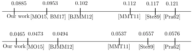
The best algorithmic paradigm that we know today for random binary linear codes is a class of algorithms called Information Set Decoding (ISD). Here, for simplicity we only compare ISD running times in the Full Distance Decoding setting, but see also Fig. 1. For all ISD algorithms the maximal run time is achieved at a rate k_n slightly below 1₂.

Fig. 1: Comparison for Full/Half Distance of our work and other algorithms.

The first ISD algorithm is due to Prange [Pra62] and achieves worst case running time 20.121n_{. This was improved by Stern and Dumer [Ste88,Dum91]} to 20.117n. Using the representation technique, May, Meurer, Thomae [MMT11] and later Becker, Joux, May, Meurer [BJMM12] further decreased the run time to 20.112n and 20.102n, respectively. The last is called BJMM algorithm and is currently asymptotically the best algorithm for decoding of random linear codes. In 2015, May and Ozerov [MO15] proposed some Nearest Neighbor (NN) search that further sped up BJMM to 20.0967n_{, which was later optimized in [BM17b]} to 20.0953n_.

Our results. As can be seen from Fig. 1, our new algorithm achieves in the Full Distance Decoding setting 20.0885n_{, which is a quite remarkable improvement} over the current state of the art. However, the improvement for the Half Distance Decoding is comparably small. As a rule of thumb, the larger the error rate, the more significant our algorithm’s improvement.

Our algorithm. ISD algorithms with representation technique such as MMT and BJMM currently use a 2-step matching process, where in the first step one does an exact matching of vectors (for eliminating representations) and in a second step one does an approximate matching via NN search. We eliminate this two-step process and perform only an approximate matching in all stages of the algorithm.

This allows us to eliminate representations less restrictive, and to use the full power of NN search in every step of our algorithm. Thus, our approximate matching is in spirit similar to the Ball Decoding approach of Bernstein, Lange and Peters [BLP11]. The heavy use of NN search might also explain the large improvement (only) in the high error-regime, where NN search can show its full strength.

This paper is organized as follows. In Section 2, we review some ISD algo-rithms. Section 3 introduces a basic version of our new algorithm, whereas the generalized version is given in Section 4. Our results are provided in Section 5.

2

Preliminaries

Syndrome Decoding. Let us start with some preliminaries on linear codes and decoding algorithms. We denote theHamming distanceof two vectorsx,y∈Fn2 by∆(x,y). The Hamming weight∆(x) ofxis defined as the Hamming distance ofxto the zero vector 0.

A linear codeCis a k-dimensional subspace of_Fn

2. Its distance is defined by

d:= minc6=c0_∈C{∆(c,c0)}. We can specifyC by a generator matrixG∈_Fk₂×n or

a parity check matrix P∈F(2n−k)×n via

C:={xG∈_Fn 2 |x∈F

k

2}or C:={c∈F n

2 |Pc=0}.

Randomlinear codes have a randomGor random P, where in both cases each matrix entry is chosen uniformly at random from _F2. For an arbitrary vector

y=c+e∈Fn2,c∈ C we define the syndrome ofyas

s:=Py=Pc+Pe=Pe. (1)

Definition 1 (Syndrome Decoding Problem).Let C be a linear code

spec-ified by some parity check matrixP ∈_F(₂n−k)×n. GivenP, an (erroneous) code-word y∈_Fn

2 and a weight ω ∈N, one has to find an error vector e∈Fn2 with

y+e∈ C and∆(e) =ω.

We call(P,s, ω)withs=Pyan instance of the Syndrome Decoding Problem. We say thate∈Fn2 solves (P,s, ω) iffs=Peand∆(e) =ω.

In Prange’s algorithm, one reduces the dimension of the search space from n

down tokvia Gaussian elimination.

In more detail, one chooses some invertibleG∈_F2(n−k)×(n−k)such thatGP = ( ¯P | In−k), where In−k is the (n−k)-dimensional identity matrix. Therefore Eq. (1) becomes

GPe= ( ¯P |In−k)e= ¯Pe0+e00=Gs=:¯s, withe= (e0,e00)∈Fk2×F n−k 2 . (2)

Thus, every instance (P,s, ω) with P ∈F2(n−k)×n of the Decoding Problem has some (non-unique) standard form ( ¯P ,¯s, ω) with ¯P ∈F2(n−k)×k such thate∈Fn2 solves (P,s, ω) iff ( ¯P |In−k)e=¯s.

Definition 2 (Standard form).For any instance(P,s, ω)∈F2(n−k)×n×F n−k 2 × Nof the decoding problem, we say that( ¯P ,¯s, ω)∈F2(n−k)×k×F

n−k

2 ×Nis a stan-dard formof (P,s, ω)if there exists some invertibleG∈F2(n−k)×(n−k) such that

GP = ( ¯P |In−k)andGs=¯s.

The underlying idea of all Information Set Decoding algorithm is to solve a dimension-reduced standard form ( ¯P ,¯s, ω) of a Decoding Problem instance in-stead of its original form (P,s, ω).

However, before transforming (P,s, ω) to its normal form one applies some column permutation π to P to enforce a special weight distribution on e = (e0,e00) ∈ _Fk

2×F n−k

2 . While Prange chooses ∆(e0) = 0, other ISD algorithms enforce ∆(e0) = pfor some parameter p≥0 (see Algorithm 1 and 2). Thus it is sufficient to find some e0 ∈ Fk2, ∆(e0) = p such that after applying π and converting to standard form the term ¯Pe0 is close to¯s, i.e.,

∆( ¯Pe0,¯s) =∆(e00) =ω−p.

Algorithm 1: _{ISD – Weight Distribution and Standard Form}

Input :P ∈F2(n−k)×n,s∈F

n−k

2 ,ω∈N

Output: e∈Fn2 withPe=sand∆(e) =ω

repeat repeat

π←random permutation onFn2

(· |Q)←π(P) (permute columns) . Q∈F(2n−k)×(n−k)

untilQis invertible

( ¯P |In−k)←Gπ(P) and¯s←Gs . G∈F(n−k)×(n−k) (e0,e00) =_ISDSolve( ¯P ,¯s, ω) .See Algorithm 2.

until(e0,e00)6=⊥

Algorithm 2: _ISDSolve

Input :P¯∈F2(n−k)×k,¯s∈F

n−k

2 , ω∈N

Output :(e0,e00)∈Fk2×Fn2−k

Parameters:choose optimal 0≤p≤ω for e0∈Fk2 with∆(e0) =pdo

e00←He0+¯s

if ∆(e00) =ω−pthen return(e0,e00)

end return⊥

Dumer’s ISD-algorithm [Dum91] introduces another parameter`and trans-formsP into a different standard form

G0P = _¯

P1 0

¯

P2In−k−`

, where ¯P1∈F2`×(k+`) and P¯2∈F2(n−k−`)×(k+`).

Set¯s:=G0s= (s1,s2)∈F`2×F n−k−`

2 . We can now write Eq. (2) as

¯

P1e (1) 1 = ¯P1e

(1)

2 +s1 and (3)

∆( ¯P2e (1) 1 ,P¯2e

(1)

2 +s2) =ω−p. (4)

splittinge0=e(1)₁ +e(1)₂ withe0,e(1)₁ ,e(1)₂ ∈Fk2+`. Hence, by Eq. (3) we have an

exact matching of ¯Pe0 and¯son ` coordinates, and by Eq. (4) an approximate

matching of the same vectors on the remaining n−k−` coordinates.

The BJMM algorithm [BJMM12] solves the exact matching of Eq. (3). In a nutshell, BJMM constructs solutions (e(1)₁ ,e(1)₂ ) for Eq. (3) using some depth-3 binary search tree. For optimizing the depth of this search tree, see [BM17b]. All candidate solutions (e(1)₁ ,e(1)₂ ) are then checked via Eq. (4).

For the approximate matching, May and Ozerov [MO15] proposed a Nearest Neighbor (NN) search algorithm that, given two lists L1, L2, finds in time sub-quadratic of the list lengths all elements (x1,x2)∈L1×L2 within some given Hamming distance∆(x1,x2). Thus, May-Ozerov NN search can be used to speed up the check of candidate solutions via Eq. (4) inside the BJMM algorithm.

Theorem 1 ([MO15]).Given two listsL1, L2with elements taken uniformly at

random from_Fn

2 and length|L1|,|L2| ≤2λn. Then for any >0one can find all

but a negligible fraction of the pairs(x1,x2)∈ L1×L2satisfying∆(x1,x2)≤γn

for some given0≤γ≤ n

2 provided that λ <1−H( γ

2)in time

2(y(λ,γ)+)n, where y(λ, γ) := (1−γ)

1−H

_H−1_(1−λ)−γ 2 1−γ

.

decoding algorithm. Whenever this condition is violated, we will choose one of the following two simple NN search algorithms Alg. 3 or 4.

Algorithm 3: NN-Enumerate-Pairs

Input :L1, L2⊂Fn2,γ

Output:L

for(x1,x2)∈L1×L2 do

if ∆(x1,x2)≤γnthen L←(x1,x2)

end

returnL

Since Algorithm 3 simply tests the distance of all pairs inL1×L2, it runs in time quadratic in the list lengths

22λn. (5)

Notice that here, as in the rest of the paper, we neglect for ease of presentation polynomial factors in the run time.

Algorithm 4: _{NN-Meet-in-the-Middle}

Input :L1, L2⊂Fn2,γ

Output:L

L02← ∅

for x2∈L2do

for e∈Fn2 with ∆(e)≤ γ 2ndo

L0₂←L0₂∪(x2+e,x2)

end end

for x1∈L1do

for e∈Fn2 with ∆(e)≤ γ 2ndo

if (x1+e,x2)∈L02 then L←(x1,x2)

end end

returnL

Recall from Theorem 1 thatL1, L2 contain random vectors from Fn2. Thus, for any pair (x1,x2)∈L1×L2 we have Pr[∆(x1,x2)≤γn] = _γnn

·2−n_{. As a} consequence, using a union bound over all pairs we can upper bound the size of the output listLfor any NN algorithm by|L| ≤ n

γn

·2(2λ−1)n_.

This in turn shows that the running time of Alg. 4 is upper bounded by

max _n

γ 2n

·2λn,

_n

γn

·2(2λ−1)n

. (6)

Since our new decoding algorithm improves the decoding with high error rate, it is best suited for attacking instances of the Learning Parity with Noise Problem (LPN).

Definition 3 (LPN). Let τ ∈[0,1₂) be some error parameter, and let s∈_Fk 2

the form

(ai, bi) := (ai,hai,si+ei), fori= 1,2, . . .

whereai∈RFk2 andei∈ {0,1} withPr[ei= 1] =τ. The goal is to recover s.

Let us denote bynthe number of samples, which can be freely chosen. We write an LPN instance as a matrix-vector tuple

(A,b)∈Fn2×k×F n

2 satisfyingAs=b+e,

wheree= (e1, . . . , en) and theithrow ofAandbrepresent theithLPN sample. Notice that A is by definition of LPN the generator matrix of a random binary linear [n, k]-code, in which we are free to choose nourselves. Thus, we can make the rate k

n arbitrarily small.

Moreover, b is a noisy codeword that is decoded to b+e with an error

e∈Fn2 of (large) expected weightE[∆(e)] =τ n. Typical parameters forτin the cryptographic setting areτ =1

4, orτ = 1 8.

3

The Depth-2 algorithm

Our Goal. As described in Section 2, many ISD algorithms like Dumer or

BJMM do an exact matching using Eq. (3) ¯P1e (1) 1 = ¯P1e

(1)

2 +s1on`coordinates, and among the candidates (e(1)<sub>1</sub> ,e(1)<sub>2</sub> ) ∈ <sub>F</sub>k+`

2 ×F k+`

2 that fulfill Eq. (3), they search for those, whose remainingn−k−`coordinates approximately match by Eq. (4).

As opposed to the BJMM algorithm, we really go back to the initial Eq. (2) ¯

Pe0+e00=¯s. Splittinge0=e₁(1)+e(1)₂ fore(1)₁ ,e(1)₂ ∈_Fk 2 yields

¯

Pe(1)₁ = ¯Pe(1)₂ +¯son alln−kbut∆(e00) =ω−pcoordinates. (7)

Our goal is to directly construct e(1)₁ ,e(1)₂ such that∆(e(1)₁ +e(1)₂ ) =pand the corresponding vectors ¯Pe(1)₁ ,P¯e(1)₂ +¯sapproximatelymatch on alln−kbutω−p

coordinates. This immediately yields a solution (e0,e00) with e00= ¯Pe0+¯sand

∆(e00) =ω−pfor the Decoding problem in standard form.

In comparison to other ISD algorithms, our vectorse(1)₁ ,e(1)₂ have length k

(like in Prange) instead ofk+`(like in Dumer, BJMM). This decreases the search space significantly. Moreover, it introduces a less restrictive weight distribution on a solution (e0,e00)∈_Fk

2×F n−k

2 , since usuallypω and we only need small weightpon the firstkcoordinates instead of the firstk+`coordinates. This in turn means that we need less iterations in Alg. 1 to find a permutation πthat fulfills our weight distribution.

Recall that by Eq. (7) our goal is to construct two listsL(1)₁ , L(1)₂ in depth 1 of a search tree containing entries

(e(1)₁ ,P¯e(1)₁ ) and (e(1)₂ ,P¯e(1)₂ +¯s) such that

∆(e0) =∆(e(1)₁ +e(1)₂ ) =pand∆(e00) =ω−p.

The two listsL(1)₁ , L(1)₂ are constructed in a recursive manner out of other lists in a search tree of some depth m that has to be optimized. In this section, we describe our algorithm for depth m= 2 only, since this already gives the main ideas.

Let us introduce some useful notion, see also Fig. 2. For any vector v =

v1. . . vn ∈ Fn2 and any positive lengths `1, . . . , `m+1 ∈ N with Pmj=1+1`i = n, we define by v[j] ∈ F`2j the projection of v onto its coordinates (

Pj−1 i=1`i + 1, . . . ,Pj

i=1`i). We also extend our notion to lists of vectors L⊂F n

2. InL[j] we project all elementsv∈Ltov[j].

Fig. 2: The projectionv[j] ofv.

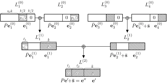
Outline of depth-2 algorithm. Here we give a high-level overview of our

construction with a search tree of depth 2. The reader is advised to follow the description via Fig. 3.

Among then−k coordinates of e00, we introduce another split into`1 and

`2 := n−k−`1 coordinates. In the final list L(2), we enforce some weight

ω1 on the first `1 coordinates of e00 = (e00_[1],e00_[2]), and the remaining weight

ω2 := ω−p−ω1 on the remaining `2 coordinates. The parameters `1, ω1 are subject to optimization.

For the construction of e00_[2] we use an NN search for the lists L(1)₁ , L(1)₂ on level 1 that gives us weightω2 on these coordinates.

In those listsL(1)₁ , L(1)₂ we furthermore enforce weightp1≥p₂ on the

coordi-nates ofe(1)₁ ande(1)₂ . The parameterp1 is again subject to optimization. Analogously we restrict to only those ¯Pe(1)₁ , ¯Pe(1)₂ +¯swhose first `1 coor-dinates have a weight ω<sub>1</sub>(1). The weight ω<sub>1</sub>(1) has to be optimized. Again, we filter out all vector sums on level 2 whose weight is not exactlyω1 on these`1 coordinates.

Fig. 3: Our depth-2 algorithm.

is analogous. In L(0)₁ we enumerate all vectors e(0)₁ ∈ Fk/2 2×0

k/2 _{with weight}

p1/2. For each of these vectors we compute ¯Pe (0)

1 . Similary, inL (0)

2 we enumerate all vectorse(0)₂ ∈0k/2×F2k/2with weightp1/2 and compute ¯Pe

(0)

2 . We then run a NN search on the first`1 coordinates to find all vector sums with weightω

(1) 1 on these coordinates. Note that the vectorse(0)₁ ande(0)₂ automatically add up to a vector of weightp1as required for listL

(1) 1 .

This concludes the high-level description of our algorithm. More details can be found in Alg. 5, which has to be used as an_ISDSolve-subroutine in Alg. 1 to obtain a full fletched ISD algorithm, including column permutation π and transformation to standard form.

List of objects. For completeness, we provide in the following a precise de-scription of the lists. For the lists of level 0, we have

L(0)₁ ={( ¯Pe(0)₁ ,e(0)₁ )∈_Fn−k 2 ×F

k/2 2 ×0

k/2_|∆(e(0)

1 ) =p1/2}, (8)

L(0)₂ ={( ¯Pe(0)₂ ,(e(0)₂ )∈_Fn−k 2 ×0

k/2 _×

Fk/2 2|∆(e (0)

2 ) =p1/2},

L(0)₃ ={( ¯Pe(0)₃ ,e(0)₃ )∈_Fn−k 2 ×F

k/2 2 ×0

k/2_|∆(e(0)

3 ) =p1/2},

L(0)₄ ={( ¯Pe(0)₄ +¯s,e(0)₄ )∈_Fn−k 2 ×0

k/2_×

Fk/2 2|∆(e (0)

4 ) =p1/2}.

Thus, all lists on level 0 have sizeS0 = _pk/2

1/2

. Note thatL(0)₁ =L(0)₃ . The lists on level 1 are constructed via NN search on the first`1coordinates such that we obtain weightω₁(1) on these coordinates. This yields

L(1)₁ ={( ¯Pe(1)₁ ,e(1)₁ )∈Fn2−k×F k 2 |∆(e

(1)

1 ) =p1, ∆(( ¯Pe (1)

1 )[1]) =ω (1) 1 },

L(1)₂ ={( ¯Pe(1)₂ +¯s,e(1)₂ )∈Fn2−k×F k 2 |∆(e

(1)

2 ) =p1, ∆(( ¯Pe (1)

By the randomness of ¯P, both lists have expected size

S1:=E[|L(1)i |] =S 2

0·Pr[weightω (1)

1 on the first`1 coordinates]

= _k/2

p1/2 2

·

`1

ω(1)₁

2`1 for i= 1,2.

Eventually, by an NN search on `2 bits for weight ω2 on the level-1 lists and subsequent filtering for weightpon the lastkcoordinates and weight ω1 on the first`1 bits, we obtain

L(2)={(e00,e0)∈Fk2×F n−k 2 |∆(e

0_{) =p,e}00_{= ¯Pe}0_{+¯s, ∆(e}00_{) =ω−p}.}

Thus, any element (e00,e0) ofL(2) _{yields a solution (e}0_,e00_{) of a Syndrome}

De-coding Problem in standard form.

Algorithm 5: Depth-2-ISDSolve

Input :P¯ ∈F2(n−k)×k,¯s∈F n−k 2 , ω

Output :(e0,e00)∈Fk2×F n−k 2

Parameters:Optimizep, ω1, `1, p1, ω (1) 1 .

Setω2=ω−p−ω1 and`2=n−k−`1.

1 Create listsL(0)_i ,i= 1,2,3,4 as defined in (8)

2 L(1)_i ←NN-Search(L(0)_2i−1, L(0)_2i ,1, ω₁(1)), i= 1,2

.NN-Search(L1, L2, i, w) performs a NN search on (L1)[i],(L2)[i]

.with target weightwwhile keeping all other coordinates.

3 L(2)←NN-Search(L(1)₁ , L(1)₂ ,2, ω2)

4 L(2)←Filter(L(2),1, ω1)) .Filter(L, i, w) filters Lfor elements

L(2)_←Filter(L(2)_{,3, p)) .with weightw on its projection inL} [i].

if |L(2)_{|>0then return (e}0_,e00_{) for some (e}00_,e0_)∈L(2)

else return⊥

Notice that Alg. 5 can only succeed to output a solution (e0,e00)6=⊥if there exists some e0 with weight psuch that ¯Pe0+ ¯s=e00 = (e00_[1],e00_[2]) with e00_[1],e00_[2]

having weightsω1 and ω2, respectively. This specific weight distribution has to be induced by the column permutationπof Alg. 1.

Definition 4. Let e ∈ Fn2 with ∆(e) = ω and k, p ∈ N. Let `1, `2 ∈ N with

`1+`2=n−k, and letω1, ω2∈Nwithω1+ω2=ω−p. We call a permutationπ goodforewith respect to(p, ω1, `1, ω2, `2), ifπ(e) = (e0,e00[1],e

00

[2])∈F k 2×F

`1

2 ×F `2

2

with

∆(e0) =p, ∆(e00_[1]) =ω1 and∆(e00[2]) =ω2.

A random permutation πis good with probability

Pπ= k p

`1

ω1

`2

ω2

n ω

It remains to show that on input a standard form Syndrome Decoding in-stance ( ¯P ,¯s, ω) that stems from a goodπ, Alg. 5 constructs a non-empty list of solutions L(2)_.

Lemma 1 (Correctness).Letebe a solution to the Syndrome Decoding Prob-lem. Let π be good for e with respect to any fixed parameters (p, ω1, `1, ω2, `2)

as given by Definition 4. Whenever we run Alg. 5 with parameters p1, ω (1) 1 ∈N

satisfying

_p

p/2

_k−p

p1−p/2

≥ 2

`1

ω1

ω1/2

`1−ω1

ω(1)₁ −ω1/2

, (9)

then on expectation we have(e00,e0)∈L(2) forπ(e) = (e0,e00).

Thus, Lemma 1 shows that any (possibly unique) solutioneto the Syndrom Decoding Problem is constructed in our sub-routine of Alg. 5 at that point in time when the full-fletched ISD Alg. 1 provides a good permutation π, under the condition that (9) holds.

Before we prove Lemma 1, we would like to show that its statement is not vacuous. Namely, there always exist p1, w

(1)

1 such that condition (9) holds. Using the Binomial Theorem, we have

n n/2

<

n X i=0

n i

= 2n <(n+ 1)

n n/2

.

This implies

2n

n+ 1 < _n

n/2

<2n.

Thus, up to a linear factor we can approximate _n/n₂

by 2n_{. Hence if we ignore}

linear factors, condition (9) collapses for the setting p1 =k/2 andw (1) 1 =`1/2 to

2p+k−p≥2`1−ω1−(`1−ω1) _{⇔ k≥0,}

which is trivially fulfilled. Thus, there always exist feasible parametersp, ω1, `1, p1, ω (1) 1 that lead to a solution when running Alg. 5. Among these feasible parameters, we will later minimize running time.

Proof (of Lemma 1). Letπ(e) = (e0,e00) be the solution of our Syndrome De-coding problem in standard form. Since we have standard form, we conclude that e00= ¯Pe0+¯sis fully determined bye0. Moreover, since we assumeπto be good,e00 is of the correct form. Thus, it suffices to show that Alg. 5 constructs the desirede0∈Fk2.

Notice that in our constructione0=e(1)₁ +e(1)₂ , and in turne(1)₁ =e(0)₁ +e(0)₂

(and analogous fore(1)₂ ).

Let us first argue that in our construction we obtain up to a polynomial factor all _pk

1

vectors e(1)₁ ∈ Fk2 on level 1. All vector sums e (0) 1 +e

the definition of e(0)₁ ,e(0)₂ different. Up to polynomial factors (denoted by ≈),

we have by standard approximation via the binary entropy function _pk/2

1/2

2

≈

22H(p1

k)k/2≈ k p1

vectorse(1)₁ that we construct.

Now let us turn to the construction ofe0with weightpon level 2 viae(1)₁ +e(1)₂

withe(1)₁ ,e(1)₂ having weightp1≥p/2. We call (e (1) 1 ,e

(1)

2 ) a representation ofe0 ife0=e(1)₁ +e(1)₂ . Notice that our desired solutione0 has

R2:=

p p/2

k−p p1−p/2

representations, (10)

since the set of 1-coordinates ine0 can be represented in _p/p₂ways as 1 + 0 or 0 + 1, and the set of 0-coordinates ine0 can be represented in _pk−p

1−p/2

ways as 0 + 0 or 1 + 1.

From an algorithmic point of view, we do not care which of theR2 represen-tations is eventually used for constructinge0. It is therefore sufficient that only 1 of theseR2representations is present inL

(1) 1 ×L

(1)

2 . Hence, for achieving minimal run time we construct only a random 1/R2-fraction of all representations such that on expectation one representation is present in L(1)₁ ×L(1)₂ , and therefore

e0 appears inL(2).

For constructing only an 1/R2-fraction, we construct on level 1 only those elements ( ¯Pe(1)₁ ,e(1)₁ )∈L(1)₁ whose first`1coordinates have weightω

(1)

1 (analo-gous for L(1)₂ ). This means that we enforce∆(( ¯Pe(1)₁ )[1])) =ω

(1)

1 . LetE be the event that there exists a representation of

e00_[1]= ( ¯Pe(1)₁ + ¯Pe(1)₂ +¯s)[1]with∆(( ¯Pe (1)

1 )[1]) =∆(( ¯Pe (1)

2 +¯s)[1]) =ω (1) 1 .

By randomness of ¯P, we have

p2,2:= Pr[E] = ω1

ω1/2

`1−ω1

ω₁(1)−ω1/2

2`1 ,

since there are a total of 2`1 _{possible representations of the forme}

[1]= ( ¯Pe (1) 1 + ¯

Pe(1)₂ +¯s)[1] out of which ω1

ω1/2

`1−ω1

ω(1)₁ −ω1/2

have the correct weight ω₁(1) for

( ¯Pe(1)₁ )[1], ( ¯Pe (1)

2 +¯s)[1] by the same argument as in Eq. (10).

Thus, the expected number of representations of e0 is R2·p2,2. Hence on expectation, we construct e0 in L(2) if R2 ·p2,2 ≥ 1, which is equivalent to

condition (9).

Complexity of the Depth-2 Algorithm. Our Alg. 5 starts with the

con-struction of lists L(0)_i , i = 1,2,3,4 (step 1) which takes time S0 = _pk/2

1/2

. By

takes time

T0:=       

2y(

log(S0 )

`1 ,

ω(1)₁

`1 )`1 if log(S0)

`1 <1−H(

ω(1)₁ 2`1 )

min{S20,max{ `1

ω₁(1)

2

·S0, S20· (`1

ω(1)₁ )

2`1 }} else

.

resulting in the listsL(1)₁ ,L(1)₂ that have expected sizeS1= _pk/2

1/2

2

·(

`1

ω(1)₁ ) 2`1 . These

lists are again combined via Nearest Neighbor search (step 3) in time

T1:=   

2y(

log(S_{1 )} `2 ,

ω₂

`2)`2 if log(S1)

`2 <1−H(

ω2

2`2)

min{S12,max{ `2

ω₂

2

·S1, S12· (`₂

ω2)

2`2 }} else

,

resulting in the final list L(2)_{. The filtering (step 4) takes timeS}

2:=|L(2)|. We only need to store the lists L(0)_i of size S0 as well as the lists L

(1) 1 , L

(1) 2 of size

S1. The total running time is

timeT = max{T0, T1, S0, S2}= max{T0, T1},

sinceT0≥S0 andT1≥S2.

Total complexity of Decoding. Alg. 5 constructs a solution iff π is good

which happens according to Definition 4 with probabilityPπ,resulting in a total expected running time ofT·P_π−1for our full-fletched ISD algorithm.

In the following Theorem 2 we provide an upper bound forT for the impor-tant setting of Full Distance (FD) Decoding, where we correct up to the distance many errors, i.e. ω=d. This serves us a first benchmark for our algorithm.

In depth 2, we achieveT ≤20.0982n _{which already improves over the bound} 20.102n _{of the original BJMM-algorithm [].}

Theorem 2. Alg. 1 in combination with Alg. 5 solves Full Distance decoding for random binary linear codes in expected time20.0982n _{using 2}0.0717n _space.

Proof. We achieve the worst-case running time at a rate of

k

n = 0.43 with relative distance ω

n =

d

n =H

−1

1−k

n

= 0.1346.

For this rate, we minimize the running time by choosing the relative weights

p

n = 0.03730, p1

n = 0.02645,

resulting in

R2= 20.09254n

representations. Furthermore, we optimize

`1

n = 0.1553 and ω1

Using condition Eq.(9) from Lemma 1, we have

ω₁(1)

n = 0.01765.

The resulting list sizes are

S0= 20.07168n, S1= 20.06741n.

The running times are

T0= 20.08483n, T1= 20.08482n,

using May-Ozerov NN search. The probability for the correct weight distribution satisfying Def. 4 is

Pπ= 2−0.01334n.

Thus the overall running time and space consumption are

T = 20.0982n and S = 20.0717n. ut

4

The Depth-

m

algorithm

Our algorithm with depth 2, as described in the previous Section 3, already illus-trates the overall idea of approximate matching, but does not yet yield improved running times compared to the BJMM algorithm. Therefore, we generalize to arbitrary depth in this section, which is mostly straight-forward but still in-cludes some subtleties how to proceed with approximate matchings - and their respective weights - over many levels of a search tree.

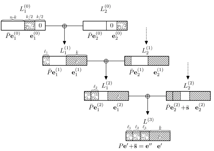
Outline of depth-malgorithm. Let us start again with a high-level overview for our algorithm with arbitrary depth m. The reader is advised to follow the description via Fig. 4 which shows the algorithm for m= 3.

In the final listL(₁m) we now split the firstn−k coordinates intom blocks instead of only 2 blocks, i.e we havee00 = (e00_[1], . . . ,e_[00_m]). Block e00_[i] has length

`i and weight ω (m)

i . The parameters`i,ω (m)

i are subject to optimization. On level 0, there are a total of 2m _{lists L}(0)

1 , . . . , L (0)

2m. The construction of the 2m−1_listsL(1)

1 , . . . , L (1)

2m−1 on level 1 out of the level-0 lists is identical to the

construction in Section 3. For the level-mlists, we have

L(0)_j

1 ={( ¯Pe

(0) j1 ,e

(0) j1 )∈F

n−k 2 ×F

k/2 2 ×0

k/2_|∆(e(0)

j1 ) =p1/2}, (11)

L(0)_j

2 ={( ¯Pe

(0) j2 ,e

(0) j2 )∈F

n−k 2 ×0

k/2_×

Fk/2 2|∆(e (0)

j2 ) =p1/2},

L(0)₂m ={( ¯Pe (0) 2m+¯s,e

(0) 2m)∈F

n−k 2 ×0

k/2_×

Fk/2 2|∆(e (0)

Fig. 4: Our algorithm for depth 3.

forj1= 1,3, . . . ,2m−1 and j2= 2,4, . . . ,2m−2. All lists on level 0 therefore have sizeS0=

k/2 p1/2

.

Starting from the level-0 lists, our algorithm combines two lists at a time using NN search in a binary tree wise fashion until we reach the final listL(m)_. On every level i = 1, . . . , m−1 we construct the first list L(₁i) via NN search on the projected lists (L(₁i−1))[i],(L

(i−1)

2 )[i] such that we obtain weight ω (i) i . We furthermore filter for weight pi on the last k coordinates and a specific weight distribution on the remaining coordinates such that we get

L(₁i)={( ¯Pe(₁i),e(₁i))∈Fn2−k×F k 2|∆(e

(i)

1 ) =pi, ∆(( ¯Pe (i)

1 )[h]) =ω (i)

h , h= 1, . . . , i}.

The other lists L(_ji), j = 2, . . . ,2i _{are created analogously. By randomness of} ¯

P the projection ( ¯Pe(₁i))[i] with weight ω (i)

i is in our construction the sum of two random vectors. For every h = 1, . . . , i−1 the projection ( ¯Pe(₁i))[h]

with weight ω(_hi) is the sum of two random vectors of specific weight ω(_hi−1).

Fixing the first vector, there are `h ω(_hi−1)

possible second vectors out of which

ω(_hi−1) ω(_hi−1)−ω(_hi)/2

`h−ω(hi−1) ω_h(i)/2

list sizes on layeriare upper bounded by

Si ≤ |{x∈Fk2|∆(x) =pi}| · Pr x∈F`i2

[∆(x) =ω_i(i)]

·

m−1 Y h=i+1

Pr x,y∈F`h2

[∆(x+y) =ω(_hi)|∆(x) =∆(y) =ω(_hi+1)]

= _k

pi

·

`i ω(_ii)

2`i · i−1 Y h=1

ω_h(i−1) ω_h(i−1)−ω_h(i)/2

`h−ω(i

−1)

h ω_h(i)/2

`h ω(_hi−1)

.

Eventually, an NN search on `m = n−k−P m−1

i=1 `i bits for weight ω (m)

m =

ω−pm−Pm_i=1−1ω (m)

i ,pm=p, on the level-(m−1) lists and subsequent filtering for weightpmon the lastkcoordinates and weightω

(m)

i for every projectione00[i],

i= 1, . . . , m−1, we obtain

L(m)={(e00,e0)∈_Fn−k 2 ×F

k

2|∆(e0) =pm,e00= ¯Pe0+¯s, ∆(e00) =ω−pm}.

Thus, any element (e00,e0) ofL(m) _{yields a solution (e}0_,e00_{) of a Syndrome}

De-coding Problem in standard form.

More details can be found in Alg. 6, which has to be used again as an ISD-Solve-subroutine in Alg. 1 to obtain a full fletched ISD algorithm.

Algorithm 6: _Depth-m_-ISDSolve

Input :P¯∈F2(n−k)×k,¯s∈F

n−k

2 , ω

Output :(e0,e00)∈Fk2×Fn −k

2

Parameters:Optimizep1, . . . , pm, ω(1m), . . . , ω (m)

m−1, `1, . . . , `m−1.

Computeωm(m)=ω−pm−Pm_i=1−1ωi(m),`m=n−k−Pm<sub>i=1</sub>−1`i. 1 Defineω(ii):=

ω(_ii+1)

2 ,i= 1, . . . , m−2.

Choose optimalω(ji)such that condition (12) holds.

2 Create listsL(0)_j ,j= 1, . . . ,2mas defined in (11).

3 L(1)_j ←NN-Search((L₂(0)_j−1)[1],(L (0) 2j)[1], ω

(1)

1 ),j= 1, . . . ,2

m−1

fori= 2, . . . , m,j= 1, . . . ,2m−ido 4 L(_ji)←NN-Search((L(₂i_j−₋1)₁)[i],(L

(i−1) 2j )[i], ω

(i)

i ) 5 L(_ji)←Filter(L_j(i), h, ω(_hi))),h= 1, . . . , i−1

L_j(i)←Filter(L_j(i), m+ 1, pi)) end

if |L(m)_{|>0then return(e}0

,e00) for some (e00,e0)∈L(m)

else return⊥

having weightω_i(m)for alli= 1, . . . , m. This specific weight distribution has to be induced by the column permutationπof Alg. 1.

Definition 5. Let e ∈ _Fn

2 with ∆(e) =ω and k, pm ∈ N. Let `1, . . . , `m ∈ N

with Pm

i=1`i=n−k, andω (m) 1 , . . . , ω

(m)

m ∈Nwith Pmi=1ω (m)

i =ω−pm.

We call a permutationπ goodfor ewith respect to pm,(ω (m)

i , `i)i=1,...,m, if

π(e) = (e0,e00_[1], . . . ,e00_[m])∈_Fk 2×F

`1

2 × · · · ×F `m 2 with

∆(e0) =pm, ∆(e00[i]) =ω (m)

i , i= 1, . . . , m.

A random permutation πis good with probability

Pπ= k pm

Qm i=1

`i ω_i(m)

n

ω

.

We now show that on input a standard form Syndrome Decoding instance ( ¯P ,¯s, ω) that stems from a goodπ, Alg. 6 constructs a non-empty list of solutions

L(m).

Lemma 2 (Correctness).Letebe a solution to the Syndrome Decoding Prob-lem. Let π be good for e with respect to any fixed parameters pm, ω

(m)

i , `i,i = 1, . . . , m as given by Definition 5. Whenever we run Alg. 6 with parameters pi, ω

(i)

j ∈N, for j= 1, . . . , i,i= 1, . . . , m−1 satisfying

_p i

pi/2

_k−p i

pi−1−pi/2

≥

i−1 Y h=1

2`h

ω(_hi) ω(_hi)/2

`h−ωh(i) ω_h(i−1)−ω_h(i)/2

, ∀i= 2, . . . , m (12)

then on expectation we have(e00,e0)∈L(m) forπ(e) = (e0,e00).

Analogous to Section 3, we can show that the settingpi =k/2 and w (i)

h =

`h/2, forh= 1, . . . , i−1,i= 2, . . . , m, yields feasible parameters for Alg. 6 that fulfill condition (12).

Proof (of Lemma 2).Letπ(e) = (e0,e00) be the solution of our Syndrome Decod-ing problem in standard form. Similar to the reasonDecod-ing in the proof of Lemma 1, it suffices to show that Alg. 6 constructs the desirede0∈_Fk

2.

Notice that in our construction e0 = e(₁m−1)+e₂(m−1), and in turn e(_ji) =

e₂(i_j−₋1)₁ +e(₂i_j−1), for allj= 1, . . . ,2i_{,i= 1. . . , m−1.}

Similar to the reasoning in the proof of Lemma 1, we obtain up to a polyno-mial factor all _pk

1

vectorse(1)_j ∈Fk2 on level 1.

We now look at the construction ofe(₁i)with weightpi on leveliviae (i−1)

1 +

all vectors on this layer and all layersi= 2, . . . , m−1 as well as the final vector

e0 on levelm. Notice that our desired vectore(₁i)has

Ri:= _p

i

pi/2

_k−p i

pi−1−pi/2

representations. (13)

It is sufficient that one of these representations is present inL(₁i−1)×L₂(i−1). For constructing only a random 1/Ri-fraction of all representations, we com-pute on level i−1 only those elements (e(₁i−1),P¯e₁(i−1)) ∈ L(₁i−1)) satisfying

∆(( ¯Pe(₁i−1))[h])) =ω (i−1)

h , h= 1, . . . , i−1 (analogous for L (i−1)

2 ). Let E be the event that there exists a representation of

( ¯Pe(₁i))[h]= ( ¯Pe (i−1) 1 + ¯Pe

(i−1)

2 )[h] with∆(( ¯Pe (i−1)

1 )[h]) =∆(( ¯Pe (i−1)

2 )[h]) =ω (i−1)

h .

forh= 1, . . . , i−1. By randomness of ¯P, we have

pi,m := Pr[E] = i−1 Y h=1

ω_h(i)

ω_h(i)/2

`h−ωh(i) ω(_hi−1)−ω_h(i)/2

2`h ,

since there are a total of 2`h _{possible representations of the form ( ¯Pe}(i) 1 )[h] = ( ¯Pe(₁i−1)+ ¯Pe(₂i−1))[h]out of which

ω(_hi)

ω(_hi)/2

`h−ωh(i) ω(_hi−1)−ω_h(i)/2

have the correct weight

ω_h(i−1) for ( ¯Pe₁(i−1))[h], ( ¯Pe (i−1)

2 )[h] by the same argument as in Eq. (13). Thus, the expected number of representations of e(₁i) isRi·pi,m. Hence on expectation, we constructe(₁i)inL₁(i)ifRi·pi,m≥1. Generalizing this condition

to all layers yields condition (12).

Complexity of Alg. 6. The listsL(0)_j , j = 1, . . . ,2m _{are created in time S} 0 (step 2). The NN search on those lists yields listsL(1)_j ,j= 1, . . . ,2m−1_{(step 3).}

Next, another NN search on the new lists returns listsL(2)_j ,j= 1, . . . ,2m−2 (step 4) which are subsequently filtered (step 5). These two steps of NN search and filtering are repeated until only one list is left. By Theorem 1 and Eq. (5), (6) the NN search layer oni= 0, . . . , m−1 takes time

Ti:=         

2y(

log(Si)

`i+1 ,

ω(_ii₊₁+1)

`i+1 )`i+1 _if log(Si)

`i+1 <1−H(

ω(_i+1i+1) 2`i+1)

min{S2 i,max{

`i+1

ω_i(₊₁i+1)

2

·Si, S2i · (`i+1

ω(_ii₊₁+1))

2`i+1 }} else

.

The filtering takes time Si on layer i= 2, . . . , m−1 andSm:=|L(m)| on layer

m.

On every leveliof our search tree we consume timeTi and store lists of size

Si. Thus, we obtain

Total complexity of Decoding. Alg. 6 constructs a solution iff π is good which happens according to Definition 5 with probabilityPπ,resulting in a total expected running time ofT·P−1

π for our full-fletched ISD algorithm.

5

Results

Syndrome Decoding Problem. The best known complexity for Full Distance

decoding is currently 20.0953n_{using BJMM in depth 4 [BM17b], whereas for Half} Distance Decoding the best known bound is 20.0473n [MO15].

As stated in Theorem 3, we improve the bound for Full Distance Decoding to 20.885n. In the Half Distance Decoding setting, we achieve a small improvement to 20.0465n.

Theorem 3. Alg. 1 in combination with Alg. 6 for m= 4solves Full Distance decoding for random binary linear codes in expected time20.0885n _using20.0736n

space. Half Distance decoding is solved in exptected time 20.0465n _{using 2}0.0294n

space.

Proof. For Full Distance Decoding we achieve the maximal running time at code rate

k

n = 0.46 with relative distance ω

n =

d

n =H

−1

1−k

n

= 0.1237.

For this code rate, we minimize the running time choosing the relative weights

p1

n = 0.00559, p2

n = 0.01073, p3

n = 0.02029, p4

n = 0.03460,

resulting in

R2= 20.01357n, R3= 20.02668n, R4= 20.06028n

representations. Furthermore we set

`1

n = 0.0366, `2

n = 0.0547, `3

n = 0.0911,

ω1

n = 0.0066, ω2

n = 0.0099, ω3

n = 0.0114, ω(3)₁

n = 0.0232.

Optimization showed that

ω(1)₁ = ω (2) 1 2 , ω

(2) 2 =

ω₂(3)

2

is a good choice which yields

ω(1)₁

n = 0.011515, ω₁(2)

ω₂(2)

n = 0.016676, ω(3)₂

n = 0.033351, ω₃(3)

n = 0.009993

using condition Eq.(12) from Lemma 2. The resulting list sizes are

S0= 20.02179n, S1= 20.03987n, S20.05939n, S3= 20.05975n.

The lists on layer 0 are combined with the NN search of Alg. 3 in time

T0= 20.04359n,

as the condition for May-Ozerov is not satisfied and Alg. 4 is less efficient in this case. On layer 1 we use Alg. 4 in time

T1= 20.07356n,

which is also the space consumption for this step. On the remaining layers, we use May-Ozerov NN search which yields

T2= 20.07365n, T3= 20.07359n.

The probability for the correct weight distribution satisfying Def. 5 is

Pπ= 2−0.01485n.

Thus the overall running time and space consumption is

T = T2

Pπ

= 20.0885n and S =T1= 20.0736n.

The complexity for Half Distance decoding can be shown analogously for a code rate

k

n = 0.47 with relative distance ω

n =

d

n =H

−1

1− k

n

= 0.06011

using the parameters

p1

n = 0.002038, p2

n = 0.003855, p3

n = 0.007490, p4

n = 0.012200

`1

n = 0.0125, `2

n = 0.0204, `3

n = 0.0350 ω1

n = 0.0012, ω2

n = 0.0019, ω1

n = 0.0019

ω(1)₁

n = 0.003581, ω₁(2)

n = 0.007161, ω(3)₁

n = 0.0062

ω₂(2)

n = 0.005906, ω(3)₂

n = 0.011812, ω₃(3)

Prange BJMM D3 BJMM+NN D3 Our D3

Fig. 5: [Pra62], [BJMM12], [MO15] and our algorithm for varying code rates _nk.

While Theorem 3 states the run time for the worst-case rate, Fig. 5 illustrates and compares the run time as a function of all constant rates k

n of our algorithm to other decoding algorithms like Prange, BJMM and BJMM with NN-search, called BJMM-NN.

We also provide the C-code for optimizing all these algorithms at https://github.com/LeifBoth/Decoding-LPN.

Fig. 6 compares in more detail for varying depthsm the complexity of our algorithm to BJMM-NN, as analyzed in [BM17b]. Here, we consider FD, HD and typical McEliece instances withk= 0.775 andω= 0.02 [BLP08].

We suspect that the strong dependency of our algorithm on the error-weight is due to the heavy reliance on Nearest Neighbor search on every layer, which needs a sufficiently large weight ω to show its strength. We will also see this effect in the case of LPN.

[BM17b] Our algorithm

mlog(T)/nlog(S)/nlog(T)/nlog(S)/n

2 0.1003 0.0781 0.0982 0.0717

3 0.0967 0.0879 0.0926 0.0647 (FD)

4 0.0953 0.0915 0.0885 0.0736 2 0.0491 0.0309 0.0488 0.0290

3 0.0473 0.0363 0.0478 0.0290 (HD)

4 0.0473 0.0351 0.0465 0.0294 2 0.0362 0.0264 0.0360 0.0260

3 0.0350 0.0280 0.0360 0.0252 (McEliece) 4 0.0350 0.0280 0.0347 0.0251

Fig. 6: Running time and memory consumption of our algorithm compared to the optimized BJMM-NN variant of [BM17b].

LPN Problem. Let us apply our algorithm to theLP Nk,τ problem (Def. 3). In LPNk,τ we have to solve a (n, k, ω)-decoding problem with expected weight

ω = τ n and fixed k. However, we are free to choose the number of samples

n, and can therefore make the code rate k_n arbitrarily small. Thus, for every fixed instance (k, τ) we minimize the running time T(n, k, τ) of our decoding algorithm over alln. The optimal number of samples for our algorithm for the cryptographically popular LPN_512,1

4-instances isn≈140.000.

In Fig. 7, we compare different decoding algorithms for directly attacking LPN_512,1

4, where we suppress polynomial overheads. Here BJMM-NN would take

2180steps, our algorithm has complexity 2169.

It is however important to stress that stand-alone decoding is not the best way to attack LPN instances. As shown by Esser, K¨ubler and May [EKM17] a combination of the BKW algorithm [GJL14] and decoding algorithm is due to its flexible memory requirements currently the best way to tackle LPN instances in practice. Here, one first uses BKW to turn LPNk,τ instances into LPNk0_,τ0

instances with reduced dimension k0 _{< kat the cost of increased error τ}0 _{> τ.}

Then in a second step, LPNk0_,τ0 is solved via decoding.

Since our decoding algorithm shows its strength for large errorsτ0_{, its seems}

like a perfect choice in such a hybrid BKW-decoding algorithm. In a typical attack on LPN_512,1

4, like the ones described in [EKM17], BKW would turn

LPN_512,1

4 into LPN117, 255

512 instances, which are subsequently decoded. The

cal-culations in Fig. 7 give us good indication that such instances with large error

LPN_512,1

4 LPN117, 255 512

log(T) log(S) log(T) log(S)

Prange [Pra62] 213 - 117

-BJMM [-BJMM12] 190 114 117 62

BJMM-NN [MO15] 180 122 117 64

Our algorithm 169 138 75 47

Fig. 7: Complexities of different decoding algorithms for LPN instances.

Fig. 8 shows the asymptotic behavior of our algorithm on LPN-instances for varying weights τ, which also illustrates the strength of our algorithm in the high error regime. Notice that the graph of our new algorithm’s complexity can be very well approximated by a line, which yields the simple formula

TLP N(k, τ) = 21.3kτ.

Prange BJMM+NN D3 Our D3

Fig. 8: Dependence on LPN errorτ of [Pra62], [MO15] and our algorithm.

References

BJMM12. Anja Becker, Antoine Joux, Alexander May, and Alexander Meurer. De-coding random binary linear codes in 2n/20: How 1 + 1 = 0 improves infor-mation set decoding. In David Pointcheval and Thomas Johansson, editors,

EUROCRYPT 2012, volume 7237 ofLNCS, pages 520–536. Springer, Hei-delberg, April 2012.

BLP08. Daniel J Bernstein, Tanja Lange, and Christiane Peters. Attacking and defending the mceliece cryptosystem. InInternational Workshop on Post-Quantum Cryptography, pages 31–46. Springer, 2008.

BLP11. Daniel J. Bernstein, Tanja Lange, and Christiane Peters. Smaller de-coding exponents: Ball-collision dede-coding. In Phillip Rogaway, editor,

CRYPTO 2011, volume 6841 of LNCS, pages 743–760. Springer, Heidel-berg, August 2011.

BM17a. Leif Both and Alexander May. Decoding linear codes with high error rate and its impact for lpn security (full version). Cryptology ePrint Archive: Report 2017/1139, 2017.

BM17b. Leif Both and Alexander May. Optimizing BJMM with nearest neighbors: full decoding in 22n/21 _{and McEliece security. International Workshop on}

Coding and Cryptography (WCC 2017), 2017.

Dum91. Ilya Dumer. On minimum distance decoding of linear codes. InProc. 5th Joint Soviet-Swedish Int. Workshop Inform. Theory, pages 50–52, 1991. EKM17. Andre Esser, Robert K¨ubler, and Alexander May. LPN decoded. In

Jonathan Katz and Hovav Shacham, editors,CRYPTO 2017, Part II, vol-ume 10402 ofLNCS, pages 486–514. Springer, Heidelberg, August 2017. GJL14. Qian Guo, Thomas Johansson, and Carl L¨ondahl. Solving LPN using

cov-ering codes. In Palash Sarkar and Tetsu Iwata, editors,ASIACRYPT 2014, Part I, volume 8873 ofLNCS, pages 1–20. Springer, Heidelberg, December 2014.

McE78. RJ McEliece. A public-key system based on algebraic coding theory, 114-116. deep space network progress report, 44. Jet Propulsion Laboratory, California Institute of Technology, 1978.

MMT11. Alexander May, Alexander Meurer, and Enrico Thomae. Decoding random linear codes in ˜O(20.054n). In Dong Hoon Lee and Xiaoyun Wang, edi-tors,ASIACRYPT 2011, volume 7073 ofLNCS, pages 107–124. Springer, Heidelberg, December 2011.

MO15. Alexander May and Ilya Ozerov. On computing nearest neighbors with applications to decoding of binary linear codes. In Elisabeth Oswald and Marc Fischlin, editors,EUROCRYPT 2015, Part I, volume 9056 ofLNCS, pages 203–228. Springer, Heidelberg, April 2015.

NIS. NIST evaluation criteria. https://csrc.nist.gov/Projects/ Post-Quantum-Cryptography. Accessed: 2017-11-24.

Pra62. Eugene Prange. The use of information sets in decoding cyclic codes. IRE Transactions on Information Theory, 8(5):5–9, 1962.

Reg05. Oded Regev. On lattices, learning with errors, random linear codes, and cryptography. In Harold N. Gabow and Ronald Fagin, editors,37th ACM STOC, pages 84–93. ACM Press, May 2005.