Polly Cracker, Revisited
?Martin R. Albrecht1, Jean-Charles Faug`ere2, Pooya Farshim3,
Gottfried Herold4, and Ludovic Perret2 1
Technical University of Denmark, Denmark 2
INRIA, Paris-Rocquencourt Centre, POLSYS Project UPMC Univ. Paris 06, UMR 7606, LIP6, F-75005, Paris, France
CNRS, UMR 7606, LIP6, F-75005, Paris, France 3
Technische Universit¨at Darmstadt, Germany
4 Ruhr-Universit¨at Bochum, Horst G¨ortz Institut f¨ur IT-Sicherheit, Germany
Abstract. We initiate the formal treatment of cryptographic constructions based on the hardness of computing remainders modulo an ideal in multivariate polynomial rings. Of particular interest to us is a class of schemes known as “Polly Cracker.” We start by formalising and studying the relation between the ideal remainder problem and the problem of computing a Gr¨obner basis. We show both positive and negative results. On the negative side, we define a symmetric Polly Cracker encryption scheme and prove that this scheme only achieves boundedCPAsecurity under the hardness of the ideal membership problem. Furthermore, we show that a large class of algebraic transformations cannot convert this scheme to a fully secure Polly Cracker-style scheme. On the positive side, we formalise noisy variants of the ideal-theoretic problems. These problems can be seen as natural generalisations of the learning with errors (LWE) and the approximate GCD problems over polynomial rings. After formalising and justifying the hardness of the noisy assumptions, we show that noisy encoding of messages results in a fullyIND-CPA-secure and somewhat homomorphic encryption scheme. Together with a standard symmetric-to-asymmetric transformation for additively homomorphic schemes, we provide a positive answer to the long-standing open problem of constructing a secure Polly Cracker-style cryptosystem reducible to the hardness of solving a random system of equations. Indeed, our results go beyond this and also provide a new family of somewhat homomorphic encryption schemes based on generalised hard problems. Our results also imply that Regev’sLWE-based public-key encryption scheme is (somewhat)
multiplicatively homomorphic for appropriate choices of parameters.
Key words.Polly Cracker, Gr¨obner bases, Learning with errors, Homomorphic encryption, Provable security.
1 Introduction
Background. Fully homomorphic encryption [53] is a cryptographic primitive which allows
per-forming arbitrary computations over encrypted data. In such a scheme, given a function f and a ciphertext c encrypting a plaintext m, it is possible to transform c into a new ciphertext c0 which encryptsf(m). From an algebraic perspective, this homomorphic feature can be seen as the ability to evaluate multivariate (Boolean) polynomials over ciphertexts. Hence, instantiating homomor-phic encryption over the ring of multivariate polynomials is perhaps most natural, although not necessarily conceptually the simplest (cf. [81]).
Indeed, let I be some ideal in P := F[x0, . . . , xn−1]. Denote an injective function mapping
bit strings to elements in the quotient ring P/I by Encode(·), and its inverse by Decode(·). If
Decode(Encode(m0) ◦ Encode(m1)) =m0 ◦ m1 for◦ ∈ {+,·}, we can encrypt a messagemas
c=f +Encode(m) for f randomly chosen in I.
?An extended abstract of this work appeared at ASIACRYPT 2011 [4]. This work also incorporates corrections that
The homomorphic features of this scheme follow from the definition of an ideal. Decryption is performed by computing remainders modulo I. The problem of computing remainders modulo an ideal was solved by Buchberger [26–28], where he introduced the notion of Gr¨obner bases, and gave an algorithm for computing such bases.
In fact, most known homomorphic schemes which support both addition and multiplication are based on variants of the ideal remainder problem over various rings. For example in [81] the ring
hpi ⊆ Z, for p an odd integer, is considered. In [53] ideals in a number field play the same role (cf. [78]). One can also view Regev’s LWE-based public-key encryption scheme [73] as well as the homomorphic encryption scheme based on it [25] in this framework. Furthermore, if we instantiate the construction in [67] over P, we can view its multiplication operation as constructing the set of cross-terms appearing in multivariate polynomial multiplication. Finally, we note that the con-struction displayed above is essentially Polly Cracker [51, 14, 63], a family of cryptosystems dating back to the early 1990s. Despite their simplicity, our confidence in Polly Cracker-style schemes has been shaken as almost all such proposals have been broken [41]. This is partially due to the lack of formal treatment of security for such schemes in the literature. In fact, it is a long-standing open research problem to propose a secure Polly Cracker-style encryption scheme [14] (cf. [52, p. 41]).
Contributions & organisation. Our contributions in this paper can be summarised as
fol-lows: (1) we initiate the formal treatment of Polly Cracker-style schemes over multivariate polyno-mial rings and characterise their security; (2) we demonstrate the impossibility of converting such schemes to fullyIND-CPA-secure schemes through a large class of transformations; (3) we introduce natural noisy variants of classical problems related to Gr¨obner bases which also generalise previ-ously considered noisy problems such as the LWE and the approximate GCD (AGCD) problems; (4) we present a new somewhat (and doubly) homomorphic encryption scheme based on these new hard problems. We detail our contributions next.
We start by giving an overview of Gr¨obner bases in Section 2. In Section 3, we formalise various problems associated with ideals in polynomials rings in the language of code-based security defini-tions [18]. In particular, we show that deciding ideal membership with overwhelming probability is equivalent to computing Gr¨obner bases for zero-dimensional ideals for certain choices of parame-ters. This allows us to introduce a symmetric variant of Polly Cracker and precisely characterise its security guarantees. In particular, we show that this scheme achieves a weaker version ofIND-CPA security where the total number of ciphertexts that the attacker can obtain is a priori bounded by a fixed polynomial. We prove this result under the assumption that computing Gr¨obner bases is hard if only a small number of polynomials are available to the attacker (Section 4). Bounded IND-CPA security is, in some sense, the best level of security that this scheme can possibly achieve: we give an attacker breaking the cryptosystem once enough ciphertexts are collected.
In order to beyond this barrier we consider constructions where the Encode() function in-troduced above is randomised. To prove security for such schemes, we consider noisy variants of the ideal membership and related problems. These can be seen as natural generalisations of the (decisional)LWEandAGCDproblems over polynomial rings (Section 6). After formalising and jus-tifying the hardness of the noisy assumptions in Section 7, we show that noisy encoding of messages can indeed be used to construct a fully IND-CPA-secure somewhat homomorphic scheme. This re-sult also implies that Regev’sLWE-based public-key scheme ismultiplicatively homomorphic under appropriate choices of parameters. Our result, together with a standard symmetric-to-asymmetric conversion for homomorphic schemes, provides a positive answer to the long-standing open problem proposed by Barkee et al. [14] asking for a Polly Cracker-style public-key encryption scheme whose security is based on the hardness of computing Gr¨obner bases for random systems of polynomials. In Section 8 we show that our scheme allows proxy encryption of ciphertexts. This re-encryption procedure can be seen as trading noise for degree in ciphertexts. In this section, we also show that our scheme achieves a limited form of key-dependent message (KDM) security in the standard model, where the least significant bit of the constant term of the key is encrypted. We leave it as an open problem to adapt the techniques of [6] to achieve full KDM security for the Polly Cracker with noise scheme. We conclude by discussing concrete parameter choices in Section 9, and give a reference implementation in Section 10.
1.1 Related work
Polly Cracker. In 1993, Barkee et al. wrote a paper [14] whose aim was to dispel the urban
legend that “Gr¨obner bases are hard to compute.” Another goal of this paper was to direct research towardssparse systems of multivariate equations. To do so, the authors proposed the most obvious dense Gr¨obner-based cryptosystem, namely an instantiation of the construction mentioned at the beginning of the introduction. In their scheme, the public key consists of a set of polynomials
{f0, . . . , fm−1} ⊂ Iwhich are used to construct an elementf ∈ I. Encryption of messagesm∈P/I
are computed as c=P
hifi+m=f +m forf ∈ I. The private key is a Gr¨obner basisG which
allows computingm=cmodI=cmodG. As highlighted in [14] this scheme can be broken using results from [38] (cf. Section 5, Theorem 6).
At about the same time, and independently of Barkee et al., Fellows and Koblitz [51, 63] pro-posed a framework for the design of public-key cryptosystems. The ideas in [51] were similar to Barkee et al.’s, but differed in two aspects. First, the polynomials generating the public ideal were derived from combinatorial or algebraic NP-complete problems (such systems were named CA-systems for “combinatorial-algebraic”). Second, the secret key was not a Gr¨obner basis of the public ideal, but rather a root of it, i.e., a Gr¨obner basis of a maximal ideal containing the public ideal. The main instantiation of such a system was the Polly Cracker cryptosystem. Fellows and Koblitz suggested several NP-complete problems, mainly based on graph-theoretic problems, for use in this context. The authors, however, did not investigate how one might generate “hard-on-average” instances of these problems with known solutions.
Not only can our constructions be seen as instantiations of Polly Cracker (with and without noisy encoding of messages), they also allow security proofs based on the hardness of computational problems related to random systems.
Homomorphic encryption. In the last decades several different approaches to construct singly
homomorphic schemes—with respect to both hardness assumptions and proofs of security—have been investigated. With respect to doubly (i.e., additively and multiplicatively) homomorphic schemes, a number of different hardness assumptions and constructions appeared in the litera-ture. These include the ideal coset problem of Gentry [53], the approximate GCD problem over the integers (AGCD) of van Dijk et al. [81], the polynomial coset problem as proposed by Smart and Ver-cauteren in [78], the approximate unique shortest vector problem, the subgroup decision problem, and the differential knapsack vector problem all of which appear in the work of Aguilar Melchor et al. [67] as well as the learning with errors problem (LWE) of Brakerski and Vaikuntanathan [25]. There is a general agreement in the community that whilst the design of fully homomorphic encryp-tion schemes is a great theoretical breakthrough, all schemes so far have remained rather imprac-tical. However, research in this direction is progressing rapidly. Recently, Gentry and Halevi [55] have been able to implement all aspects of Gentry’s scheme [53], including the bootstrapping step. In this work the authors also improve on the work of Smart and Vercauteren [78]. Later, Gentry, Halevi, and Smart implemented AES homomorphically [57]. However, the bootstrapping step still renders somewhat homomorphic schemes impractical (cf. [70]). Hence, some recent constructions aim to avoid it [24, 54] and work is ongoing to improve this step [56].
Recently and independently of this work, Brakerski and Vaikuntanathan [25] gave an encryp-tion scheme, SH, based on the LWE problem that can be seen as a linear variant of our noisy Polly Cracker scheme. Furthermore, the technique we propose in Section 8 was also independently proposed in this work. However, in contrast to our work, the authors of [25] have an explicit non-algebraic perspective. Also, a second scheme, BTS, was also proposed in [25], and it achieves full
homomorphicity based on a “dimension-modulus reduction” technique, while our work only yields a somewhat homomorphic encryption scheme. We note that this technique also applies to our con-structions. Finally, we note that improvements such as those proposed in [34] immediately apply to our constructions (which generalise the constructions considered there).
The main difference between our work—which can be seen as an instantiation of Gentry’s ideal coset problem—and previous work is that we base the security of our somewhat homomorphic scheme onnew computational problems related to ideals over multivariate polynomial rings which
generalisepreviously considered problems [25, 81]. Furthermore, our construction in Section 7 can be seen as a generalisation of a number of known schemes and their underlying hardness assumptions. As such, our work does not improve on such constructions in terms of efficiency, but provides a unified perspective on previous schemes and problems.
MQ cryptography. Our work can also be seen in relation to public-key cryptosystems based on the hardness of solving multivariate quadratic equations (MQ). A difference is that our con-structions enjoy strong reductions to the well-known (hard) problem of solving arandom system of equations, whereas the bulk of work inMQcryptography relies on heuristic security arguments [84, 68, 22, 39]. Moreover, our work is more in the direction of research initiated by Berbain et al. [19, 7], who proposed a stream cipher whose security was reduced to the difficulty of solving a system of random multivariate quadratic equations over F2. Note also that the concept of adding noise
design of an authentication scheme. Similarly, this idea was recently utilised in a novel construc-tion [62] where the public key is noise-free but ciphertexts are noisy. We remark that, in contrast to our work, the hardness of the scheme described in [62] is based on the difficulty of solving a system of nonlinear equations which is somewhat structured (the coefficients of the nonlinear parts of the polynomials are chosen according to a discrete Gaussian). Also, our work presents a gen-eral treatment of problems related to ideals over multivariate polynomials—both with and without noise—and aims to provide a formal basis to assess the security of cryptosystems based on such problems.
2 Basics of Gr¨obner Bases
In this section we recall some basic definitions and results related to Gr¨obner bases [28, 26, 27]. For a more detailed treatment we refer the reader to [36].
Notation.We write x←y for assigning valuey to a variable x, and x←$ X for samplingx from
a set X uniformly at random. If Ais a probabilistic algorithm we write y←$A(x1, . . . ,xn) for the
action of running A on inputs x1, . . . ,xn with uniformly chosen random coins, and assigning the
result toy. For a random variableXwe denote by [X] the support ofX, i.e., the set of all values that Xtakes with nonzero probability. We use PPT for probabilistic polynomial-time. We call a function
(λ) negligible if|(λ)| ∈λ−ω(1). We say a functionf(λ) is overwhelming if 1−f(λ) is negligible. We
say that a function spaceFunSp(P) and a message spaceMsgSp(P), both parameterised byP, are compatible if for any possible value of P and for anyf ∈FunSp(P), the domain off is MsgSp(P). We also denote by ω the matrix multiplication exponent (a.k.a. the linear-algebra constant) as defined in [82, Chapter 12]. We recall [83, 80] that ω∈[2,2.3727].
We consider a polynomial ring P = F[x0, . . . , xn−1] over some finite field (typically prime),
some degree-compatible monomial ordering on the elements of P with xi > xj if i < j, and a
set of polynomials f0, . . . , fm−1. We denote by M(f) the set of all monomials appearing in f ∈P
and extend this definition to sets of polynomials in the natural way. By LM(f) we denote the
leading monomial appearing inf ∈P according to the chosen term ordering. We denote byLC(f)
the coefficient of LM(f) in f, and set LT(f) := LC(f)·LM(f). We denote by P<d the set of polynomials of degree< d (and analogously for >,≤,≥, and = operations). We define P=0 as the underlying field, including 0∈F. We define P<0 as zero. Finally, we denote by M<m the set of all
monomials< mfor some monomialm(and analogously for>,≤,≥, and = operations). We assume the usual power-product representation for elements of P.
Definition 1 (Generated ideal). Let f0, . . . , fm−1 ∈P be polynomials. The set
I =hf0, . . . , fm−1i:= (m−1
X
i=0
hifi|h0, . . . , hm−1∈P )
is called the ideal generated by f0, . . . , fm−1.
It is known that every ideal I of P is finitely generated, i.e., there exists a finite number of polynomialsf0, . . . , fm−1 inP such thatI=hf0, . . . , fm−1i. A Gr¨obner basis of an ideal is a set of
Definition 2 (Gr¨obner basis). LetI be an ideal ofF[x0, . . . , xn−1]and fix a monomial ordering. A finite subset G= {g0, . . . , gm−1} ⊂ I is said to be a Gr¨obner basis of I if for any f ∈ I there exists a gi∈G such that
LM(gi)|LM(f).
Remark.We note that for the vector space Fn, the notion of a Gr¨obner basis coincides with that of a row echelon form, and Gr¨obner basis algorithms (see below) reduce to Gaussian elimination. For univariate polynomial rings, e.g., F[x] and Z[x], the notion of a Gr¨obner basis coincides with greatest common divisor, and running a Gr¨obner basis algorithm computes the GCD.
It is possible to extend the polynomial division algorithm to multivariate polynomials: we write
r =f modG when r is a possible result of applying the multivariate division algorithm on f and
G for the given monomial ordering. It holds that f =Pmi=0−1higi+r with M(r)∩ hLM(G)i =∅.
WhenGis a Gr¨obner basis,r is unique and is called thenormal form off with respect to the ideal
I. In particular, we have that f modI =f modG = 0 if and only if f ∈ I. Given P and I, we can define the quotient ring P/I. By abuse of notation, we write f ∈P/I iff modI =f where the last equality is interpreted over the elements ofP. That is, we identify elements of the quotient
P/I with their minimal representation inP.
As defined above, a Gr¨obner basis is not unique. For instance, we can multiply any polynomial of a Gr¨obner basis by a nonzero constant. However, given any Gr¨obner basis we can compute the uniquereduced Gr¨obner basis in polynomial time via ReduceGB(·) given in Algorithm 1.
Definition 3 (Reduced Gr¨obner basis). A reduced Gr¨obner basis for an ideal I ⊂ P is a Gr¨obner basis G such that: (1) LC(g) = 1, for all g∈G, and (2) ∀g∈ G,6 ∃ m∈M(g) such that m is divisible by some element of LM(G\ {g}).
Algorithm 1:ReduceGB(G)
1 begin
2 G˜←∅;
3 whileG6=∅do
4 f←the smallest element ofGaccording to the term ordering; 5 G←G\ {f};
6 if LM(f)6∈ hLM( ˜G)ithen 7 G˜←G˜∪ {LC(f)−1·f};
8 return
h
hmod ˜G\{h} |h∈G˜i;
Buchberger [26] proved that in order to compute a Gr¨obner basis from a given ideal basis, it is sufficient to consider so-called S-polynomials. From such a basis, it is easy to compute the (unique) reduced Gr¨obner basis using Algorithm 1.
Definition 4 (S-polynomial). Let f, g ∈F[x0, . . . , xn−1]be nonzero polynomials. – Let LM(f) =Qni=0−1x
αi
i and LM(g) = Qn−1
i=0 x βi
i , with αi, βi∈N, denote the leading monomials of f and g respectively. For every 0 ≤ i < n set γi := max(αi, βi) and denote by xγ the polynomial Qni=0−1xγi
– The S-polynomial of f and g is defined as
S(f, g) = x
γ
LT(f)
·f − x γ
LT(g) ·g.
Buchberger showed that a basis is a Gr¨obner basis if all S-polynomials “reduce to zero.”
Definition 5 (Reduction to zero). Fix a monomial order in P and letG={g0, . . . , gs−1} ⊂P be an unordered set of polynomials and let t be a monomial. Given a polynomial f ∈P, we say f has at-representation with respect to ≤ and Gif f can be written as
f =a0g0+· · ·+as−1gs−1,
such that whenever aigi 6= 0, we have aigi ≤t. Furthermore, we write that f −→
G 0 (“f reduces to zero”) if and only if f has an LM(f)-representation with respect to G.
Note thatf modG= 0 implies that f −→
G 0 while the converse is not necessarily the case.
Theorem 1 (Buchberger’s criterion). A basis G={g0, . . . , gs−1} for an idealI is a Gr¨obner basis if and only if for all i6=j we have S(gi, gj)−→
G 0.
Proof. See [16, p.211ff]. ut
Theorem 1 leads to an algorithm [26] which computes a Gr¨obner basis by constructing and reducing S-polynomials. However, this algorithm—Buchberger’s algorithm—spends most of its time reducing elements to zero, a computation which is of no use. Buchberger also proposed two criteria which tell usa priori whether the S-polynomial of two polynomials reduces to zero. We make use of the first criterion in this work:
Theorem 2 (Buchberger’s first criterion). Let f, g∈P be such that
LCM(LM(f),LM(g)) =LM(f)·LM(g), i.e.,f and g have disjoint leading terms. Then S(f, g) −→
{f,g}0.
Proof. See [16, p.222ff]. ut
From this, we obtain the following corollary.
Corollary 1. A set {g0, . . . , gn−1} ⊂ P with LM(gi) = xdii with di ≥ 0 for all i,0 ≤ i < n is a Gr¨obner basis.
All ideals considered in this work are zero-dimensional, i.e., their associated varieties have finitely many points. The following lemma establishes the equivalence between various statements about zero-dimensional ideals. This result will be required to analyse some algorithms introduced in Section 3.
Lemma 1 (Finiteness criterion). Let I = hf0, . . . , fm−1i ⊂ P := F[x0, . . . , xn−1] be an ideal. The following conditions are equivalent.
2. For anyi∈ {0, . . . , n−1}, we have I ∩F[xi]6=∅.
3. For anyi∈ {0, . . . , n−1}, there existsgi ∈ I such that LM(gi) =xdii withdi >0. 4. The set of monomialsS(I) :=M(P)\ {LM(f)|f ∈ I}is finite.
5. The F-vector space P/I is finite-dimensional and a basis is given by S(I).
As soon as one of these conditions holds true, then we call the ideal I zero-dimensional. Moreover, the number of solutions counted with multiplicities in the algebraic closure ofFis exactly the cardinal
of S(I) which is the dimension of the vector space P/I.
Proof. See [36, p.234ff]. ut
We will be using reduction modulo an ideal to sample polynomials from some ideal. The following lemma will be helpful to assert that this sampling is uniform.
Lemma 2. Let I ⊂ P = Fq[x0, . . . , xn−1] be an ideal with a degree-compatible term ordering ≤. Then any element f ∈P withdeg(f) =bhas a unique representationf = ˜f+r withf˜∈ I andr∈ P/I where deg( ˜f)≤b and deg(r)≤b. In particular, if M(P≤b/I) is the set of monomials in P/I with degree at mostb, then for any f˜∈ I≤b there areqs elementsfi inP≤b withf˜=fi−(fi modI) and s=|M(P≤b/I)|.
Proof. Given f we recover the uniquer by computingf modG by a standard fact about Gr¨obner bases and get ˜f = f −r. Since P has a degree-compatible ordering, r has degree at most b. To prove the second claim, note that the monomials in P≤b span an n+bb
-dimensional vector space
V overFq. The monomials inP/I up to degree b span a subspace ofV of dimension |M(P≤b/I)|,
from which the claim follows. ut
3 The Gr¨obner Basis and Ideal Membership Problems
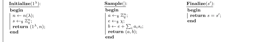
In this section we formalise various problems associated with Gr¨obner bases. To do so, we use the code-based game-playing language [18]. Each game has anInitializeand aFinalize procedure. It also has specifications of procedures to respond adversary’s various oracle queries. A game Game is run with an adversary Aas follows. First Initializeruns and its outputs are passed toA. Then
A runs and its oracle queries are answered by the procedures of Game. When A terminates, its output is passed toFinalize which returns the outcome of the gamey. This interaction is written as GameA =⇒ y. In each game, we restrict our attention to legitimate adversaries, which are defined specifically for each game.
Following [37], we definea computational polynomial ring scheme. This is a general framework allowing to discuss in a concrete way the different families of rings that may be used in cryptographic applications. More formally, a computational polynomial ring schemeP is a sequence of probability distribution of polynomial ring descriptions (Pλ)λ∈N. A polynomial ring description1 P specifies
various algorithms associated withP such as computing the ring operations, sampling of elements, testing membership, encoding of elements, ordering of monomials, etc. We assume each polynomial ring distribution is over n=n(λ) variables, for some polynomialn(λ), and is over a finite field of prime sizeq(λ).
For q a prime, there is a one-to-one correspondence between ideals I ⊂ Fqn[x0, . . . , xn−1] on
polynomial rings over finite extension fields and over prime fields J ⊂ Fq[x0, . . . , xn−1, α]: map
1
a root of Fqn to α and add the characteristic polynomial of Fqn to the generating basis. Hence,
finite extension fields are covered by this definition. The ringZ[x0, . . . , xn−1] is not covered by our
definition for brevity, but it can easily be generalised [16, Ch. 10].
Once P is given and a concrete ring P is sampled, one can define various Gr¨obner basis gen-eration algorithms on P. In this work we denote by GBGen(1λ, P, d, `) any PPT algorithm which outputs a reduced Gr¨obner basis G for some zero-dimensional ideal I ⊂ P such that the last `
elements of Ghave degree dand the remaining elements have degree 1 and such that (P\ I)≤b is
not empty. Of particular interest to us is the Gr¨obner basis generation algorithm shown in Algo-rithm 2 called GBGendense(·). Throughout this paper we assume an implicit dependency of various
parameters associated withP on the security parameter. Thus, we dropλto ease notation. Finally, we always assume thatLM(G) and henceS(I) is fixed byGBGen(·) for eachλ, and thus is known.
Algorithm 2:AlgorithmGBGendense(1λ, P, d, `)
1 begin
2 if d= 0then return{0}; 3 for0≤i < ndo
4 if i > n−`−1then
5 gi←xdi;
6 else
7 gi←xi;
8 formj∈M<LM(gi) do
9 cij←$Fq;
10 gi←gi+cijmj;
11 returnReduceGB({g0, . . . , gn−1});
We note that using Buchberger’s First Criterion in Algorithm 2 is a special case of using Macaulay’s trick [69].
Note that GBGendense(·) for d= 1 or any d >1 with ` = 0 captures the usual case of a set of
polynomials which have a (unique) common root in the base field, and where LM(gi) =xi for all i,0 ≤ i < n. This case is common in cryptographic applications such as algebraic cryptanalysis, e.g., [46, 35, 40, 48, 44, 1, 2, 21, 47, 49], and is well studied. The next lemma—which is an easy conse-quence of Corollary 1—establishes thatGBGendense(·) returns a Gr¨obner basis with dim(P/I) =d`. Lemma 3. Let G={g0, . . . , gn−1} ⊂P =F[x0, . . . , xn−1] be the set of polynomials defined as
gi:=xdii+ X
cijmj,
where the sum is overmj ∈M
<xdii ,cij ∈F, andi= 0, . . . , n. ThenGis a Gr¨obner basis for the zero-dimensional idealhg0, . . . , gn−1i. Additionally, the dimension of theFq-vector spaceP/hg0, . . . , gn−1i is Qni=0−1di.
Proof. The Gr¨obner basis property follows from Corollary 1. Clearly,S(I) =M(P)\ {LM(f)|f ∈ I}is the set of all monomials of the formQnj=0−1xγj
j where allγj < dj. Since there areQni=0−1di such
Denote Q = P≤b/I for b some fixed parameter and note here that P≤b/I = (P/I)≤b, since the
monomial order sorts by total degree first. In this work we are mainly interested in the case where
Qhas polynomially many elements. In this case we require`to be a constant but allowq to depend on λ. We note, however, that larger quotients are permitted by our definitions.
We now formally define the Gr¨obner basis problem, which is the problem of computing the Gr¨obner basis for some ideal I given a set of polynomialsf0, . . . , fm−1∈ I.
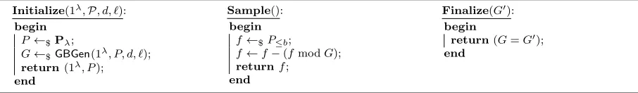
Definition 6 (The Gr¨obner basis (GB) problem). The Gr¨obner basis problem is defined through game GBP,GBGen(·),d,`,b,m shown in Figure 1. The advantage of a PPT algorithm A in solving the GBproblem is defined by
AdvgbP,GBGen(·),d,`,b,m,A(λ) := PrhGBAP,GBGen(·),d,`,b,m(λ)⇒Ti.
An adversary is legitimate if it calls theSampleprocedure described in Figure 1 at mostm=m(λ)
times.
Initialize(1λ,P, d, `):
begin P ←$Pλ;
G←$GBGen(1λ, P, d, `);
return(1λ, P);
end
Sample(): begin
f←$P≤b;
f←f−(fmodG); returnf;
end
Finalize(G0): begin
return(G=G0); end
Fig. 1.Game GBP,GBGen(·),d,`,b,m.
It follows from Lemma 2 that the Sample procedure in Figure 1 returns elements of degree ≤ b
which are uniformly distributed in hGi≤b. We note that usually we must require b ≥ d in order
to exclude the trivial case where Sample always returns zero or elements independent of some elements of the Gr¨obner basis.
We recall that given a Gr¨obner basis G of an ideal I, r = f modI = f modG is the normal form of f with respect to the ideal I. We sometimes drop the explicit reference to I when it is clear from the context which ideal we are referring to, and simply refer to r as the normal form of f. Furthermore f ∈ I if and only if r = 0. This is the well-known ideal membership problem formalised below. We mention that solving this problem was the original motivation which led to the discovery of Gr¨obner bases [26].
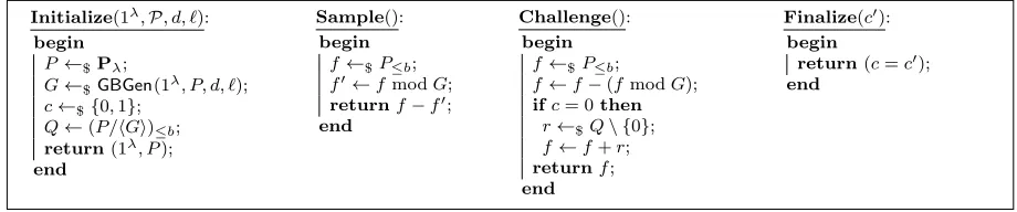
Definition 7 (The ideal membership (IM) problem).The ideal membership problem is defined through gameIMP,GBGen(·),d,`,b,mshown in Figure 2. The advantage of a PPT algorithmAin solving
IM is defined by
AdvimP,GBGen(·),d,`,b,m,A(λ) := 2·Pr
h
IMAP,GBGen(·),d,`,b,m(λ)⇒T
i −1.
An adversary is legitimate if it calls theSampleprocedure described in Figure 2 at mostm=m(λ)
times.
Initialize(1λ,P, d, `):
begin P ←$Pλ;
G←$GBGen(1λ, P, d, `);
c←${0,1};
Q←(P /hGi)≤b;
return(1λ, P);
end
Sample(): begin
f←$P≤b;
f0←fmodG; returnf−f0; end
Challenge(): begin
f←$P≤b;
f←f−(fmodG); ifc= 0then
r←$Q\ {0}; f←f+r; returnf; end
Finalize(c0): begin
return(c=c0);
end
Fig. 2.GameIMP,GBGen(·),d,`,b,m.
We define a game IM0P,GBGen(·),d,`,b,m similarly to the game in Figure 2 except that the zero element is allowed when c = 0 in the Challenge procedure (i.e., r←$ Q\ {0} is replaced by
r←$Q). The advantage of any adversary A in a modifiedIM0 game can be easily related to that in theIM game.
Lemma 4. For any adversary A,
AdvimP,GBGen(0 ·),d,`,b,m,A(λ) =
1− 1 |Q|
·AdvimP,GBGen(·),d,`,b,m,A(λ).
Proof. Let pbe the probability that A outputs 0 when the remainder of the challenge polynomial modulo Gis zero. Letp0 denote the probability that Aoutputs 1 when this remainder is nonzero. We have:
2·Pr[Awins the IMgame]−1 =p+p0−1,
2·Pr[Awins the IM0 game]−1 =p+ 1
|Q|(1−p) +
1− 1 |Q|
p0−1 =
1− 1 |Q|
·(p+p0−1).
The lemma follows. ut
We show below that under certain conditions the GB and IMproblems are equivalent. Informally, the reduction of theGBproblem to theIMproblem works as follows. Consider an arbitrary element
giin the Gr¨obner basisG. We can writegiasxdii−g˜i for some ˜gi< gi. Now, assumexdii−ri is in the
ideal and thatri < xdi
i , i.e.,LM(x di
i −ri) =x di
i andx di
i −ri∈ hGi. To find such anriwe exhaustively
searchQand hence require|Q|= poly(λ). Repeat this process for allxdi
i and accumulate the results xdi
i −ri in a list ˜G. The list ˜Gis a list of elements in hGiwithLM( ˜G) =LM(G) which implies that
˜
G is a Gr¨obner basis. We note that this is the core idea behind the FGLM algorithm [45] which allows to efficiently change the ordering of a Gr¨obner basis given access to an oracle computing normal forms with probability 1 (and also “Bulygin’s attack” in a different context [29]).
Lemma 5. (IM overwhelmingly easy =⇒ GB overwhelmingly easy) Suppose the quotient size |Q| is polynomial in λ. Then for any PPT adversary A against the IM problem, there exists a PPT adversary B against the GB problem such that
1−poly(λ)· 1−AdvimP,GBGen(·),d,`,b,m,A(λ)
(GB easy =⇒ IM easy) Conversely, for any PPT adversary A against the GB problem, there exists a PPT adversary B against the IM problem such that
AdvgbP,GBGen(·),d,`,b,m,A(λ)≤AdvimP,GBGen(·),d,`,b,m,B(λ).
Proof. Let us writePAim-0 (resp.,PAim-1) for the success probability of any algorithmA against the IMproblem conditioned on the event c= 0 (uniform challenge) (resp.,c= 1). Various parameters are implicitly understood from the context. By the definition of advantage, we have
AdvPim,GBGen(·),d,`,b,m,A=PAim-0+PAim-1−1.
Now, to prove the first statement, we construct an algorithm B against the GBproblem based on an algorithmA against theIM problem. This algorithm is described in Algorithm 3.
Algorithm 3:GBadversaryB from IMadversaryA
1 begin
2 Breceives (1λ, P); 3 G˜←∅;
4 queryGB.Sample() to getf0, . . . , fm−1;
5 queryGB.Sample() to getf; 6 form∈LM(G)do
7 forb∈P/I do
8 runA(1λ, P) as follows: 9 if AqueriesIM.Sample()then
10 answerA’sith query withfi;// we reuse fi between different runs of A.
11 if AqueriesIM.Challenge()then
12 ˜gi=m−b;
13 returnf+ ˜gi;
14 if AcallsIM.Finalize(c0)then 15 if c0= 1then// gi˜ likely in I
16 G˜←G˜∪ {˜gi};
17 break;
18 callGB.Finalize( ˜G);
We lower-bound the probability that algorithm B returns the correct Gr¨obner basis based on the success probability ofA. Note that if all ofA’s answers are correct, thenB’s output will be the Gr¨obner basis. Applying the union bound, we derive an upper bound on the failure probability of
B by bounding the failure probability of A in each invocation. Let ε =PAim-0+PAim-1 −1 be A’s advantage. Now consider invocations ofAwith ˜gi =m−b∈ I withinB. Then on such a query,Ais
run in an environment with the challenge bit being 1. By definition, the probability ofA’s failure in this case is 1−PAim-1. Now consider invocations with ˜gi 6∈ I. Since we iterate over all remainders, the
average (over the choice ofb, such that ˜gi 6∈ I) failure probability for such invocations is 1−PAim-0. The union bound leads to an upper bound of
on the failure probability of B, which in turn can be upper bounded by
|LM(G)|(|Q| −1)(2−PAim-1−PAim-0) =|LM(G)|(|Q| −1)(1−ε),
as desired.
Finally, it is easy to see that Algorithm 3 runs in polynomial time. The outer loop is repeated
|LM(G)|and the inner loop |P/I| both of which are poly(λ). Algorithm B makes one additional query to Samplecompared toA and hence needs m+ 1 samples.
Algorithm 4:IMadversaryB from GBadversaryA
1 begin
2 Breceives (1λ, P);
3 QueryIM.Challenge() to geth; 4 RunA(1λ, P) as follows: 5 if AqueriesGB.Sample()then 6 queryIM.Sample() to getf; 7 returnf;
8 if AcallsGB.Finalize(G0)then
9 if G0 is a red. Gr¨obner basis with the correct leading monomials then
10 r←hmodG0;
11 callIM.Finalize 1−(r= 0);
12 else
13 c0←${0,1};
14 callIM.Finalize(c0);
For the second statement, we construct B as in Algorithm 4. We use A to find a candidate Gr¨obner basis G0. If G0 = G we can compute the remainder r modulo the ideal spanned by the basis in polynomial time (cf. [36, p. 82]) and check ifr = 0. SoB will be successful wheneverAis. By definition, the advantage ofB is given by
AdvimP,GBGen(·),d,`,b,m,B(λ) = 2·Pr [B successful]−1
= 2 Pr [Bsuccessful| A successful]−12
·Pr [A successful] + 2 Pr [B successful| A not successful]−1
2
·Pr [Anot successful].
The first summand is exactly what we need, so to finish the proof we need to show that the second summand is non-negative. This means, it remains to show that ifG0 6=G, then B still has a non-negative advantage, i.e., B guesses cwith probability at least 1/2. Indeed, ifG0 does not have the correct form,B simply guesses the bitc(leading to a zero advantage). Moreover, ifG0 has the right form, reduction modulo G0 gives rise to an Fq-linear map mG0 :P≤b −→ Q,f 7→ f modG0. Since
surjective linear maps preserve uniform distributions on finite-dimensional vector spaces, it follows that
Pr
f←$P≤b
[mG0(f) = 0] = 1
|mG0(P≤b)| and f←Pr$I≤b
[mG0(f) = 0] = 1
Since I≤b⊆P≤b, we get
Pr
f←$P≤b
[mG0(f) = 0]≤ Pr
f←$I≤b
[mG0(f) = 0].
Now, let
p0 := Pr
f←$P≤b
[f ∈ I≤b] and p1 := Pr f←$P≤b
[f ∈P≤b\ I≤b],
wherep1 6= 0 since the quotient has positive dimension. Finally, letA be the event “mG0(f) = 0.”
Then, since
Pr
f←$P≤b
[A] =p0· Pr
f←$I≤b
[A] + p1· Pr
f←$P≤b\I≤b
[A],
we get
p0· Pr
f←$I≤b
[A] +p1· Pr
f←$P≤b\I≤b
[A]≤ Pr
f←$I≤b
[A]
⇐⇒ p1· Pr
f←$P≤b\I≤b
[A]≤(1−p0)· Pr f←$I≤b
[A]
⇐⇒ p1· Pr
f←$P≤b\I≤b
[A]≤p1· Pr
f←$I≤b
[A]
⇐⇒ Pr
f←$P≤b\I≤b
[A]≤ Pr
f←$I≤b
[A].
u t
Remark. Lemma 5 only proves a weak form of the equivalence between IM and GB. That is,
for Lemma 5 to be meaningful we require that the IM adversary returns the correct answer with
overwhelming probability. First, this is due to the restriction that Sample can only be called a bounded number of times, and thus we cannot amplify the success probability of theIMadversary through repetition. We note that it is possible to prove a stronger statement than Lemma 5 for
d= 1 using the re-randomisation technique from [20] (cf. [5]). Second, Lemma 5 does not address “structural errors” when d >1, e.g., anIMoracle which decides based on partial information only. For example, assumeG= [x0+s0xn−1, x1+s1xn−1, . . . , x2n−1+sn−1xn−1] wheresi←$Fq. This is
a valid Gr¨obner basis generated by an algorithm satisfying the requirements forGBGen(·). We have thatS(I) ={xn−1,1} and by construction anyf ∈P with a nonzero constant coefficient is not an
element of I =hGi. Hence, it is easy—although not overwhelmingly so—to solve the IM problem by considering the constant coefficient only. On the other hand, theGBproblem is still assumed to be hard, as it requires to recover all si.
3.1 Hardness assumptions
It is well known [15] that the worst-case complexity of the best algorithms of Gr¨obner bases com-putation is doubly exponential in the number of variables. However, in this work we are concerned with polynomial systems over finite fields, which do not achieve this worst-case complexity. In par-ticular, we consider zero-dimensional ideals, i.e., ideals with a finite number of common roots. In this section, we recall a number of complexity results for these type of systems.
Definition 8 (Macaulay matrix). For a set of m polynomials f0, . . . , fm−1 ∈ P we define the Macaulay matrixMacaulayd,m of degree das follows. List “horizontally” all the degree ≤dmonomials from largest to smallest sorted by some fixed monomial ordering. The smallest monomial comes last. Multiply each fi by all monomials ti,j of degree d−di where di = deg(fi). Finally, construct the coefficient matrix for the resulting system:
Macaulayd,m :=
monomials of degree ≤d
(t0,0, f0)
(t0,1, f0) (t0,2, f0)
.. .
(t1,0, f1) .. .
(tm−1,0, fm−1)
(tm−1,1, fm−1) .. . .
Theorem 3. Let F ={f0, . . . , fm−1} be a set of polynomials in P. There exists a positive integer D for which Gaussian elimination on all Macaulayd,m matrices for d= 1, . . . , D computes a Gr¨obner basis of hFi.
The F4 algorithm [42] can be seen as another way to use linear algebra without knowing an a
priori bound: it successively constructs and reduces matrices until a Gr¨obner basis is found. The same is true for the F5algorithm when considered in “F4-style” [9, 3]. Consequently, the complexity
is bounded by the degreeD and the number of polynomials considered at each degree. For F5 [43]
and the matrix-F5 variant [50] we know that under some regularity assumptions all matrices have
full rank which implies that the number of rows in the matrix is bounded by the number of columns. The number of monomials up to some degree d is bounded by n+dn and thus when considering some degree dthe number of rows and columns of the matrices considered by F5 is also bounded
above by n+dd
. Thus, knowing the degree up to which F5has to compute provides an upper bound
on the complexity of Gr¨obner bases. For this, the following definition [12] is useful.
Definition 9 (Semi-regular sequence of degree D).Letf0, . . . , fm−1 be homogeneous polyno-mials inP whose degrees ared0, . . . , dm−1 respectively. We call this system a semi-regular sequence of degree D if:
1. hf0, . . . , fm−1i 6=F[x0, . . . , xn−1].
2. For all0≤i < m and g∈F[x0, . . . , xn−1],
(deg(g·fi)< D and g·fi ∈ hf0, . . . , fi−1i) =⇒ g∈ hf0, . . . , fi−1i. We call D the degree of semi-regularity of the system.
Definition 10 (Semi-regular sequence [12]). Let m > n, and f0, . . . , fm−1 be homogeneous polynomials of degreebinP generating an idealI. The system is said to be a semi-regular sequence if the Hilbert series [16] of I with respect to the degree reverse lexicographical order is
HI(z) = X
k≥0
ckzk=
Hence, for semi-regular sequences the degree of semi-regularity of the system is given by the index of the first non-positive coefficient of HI(z).
This notion can be extended to affine polynomials by considering their homogeneous compo-nents of highest degree. It is conjectured that random systems are semi-regular with overwhelming probability. For semi-regular sequences, we have the following complexity result for F5 [12, 13, 11]. Theorem 4. Assuming that F is a semi-regular sequence, the complexity of the currently best known algorithm (i.e., F5) to solve the Gr¨obner basis problem is given by
O
n+D D
ω
where2≤ω <3is the linear algebra constant, andDis the degree of semi-regularity of the system.
Asymptotic bounds for the degree of semi-regularity for semi-regular sequences of degree 2 can be found in [12]. These bounds for the degree of regularity lead to the following complexity estimates for Gr¨obner basis computations.
Corollary 2. Let c≥0. Then for m(λ) =c·n(λ) (resp., m(λ) =c·n(λ)2) quadratic polynomials in some ideal I ⊂ Fq[x0, . . . , xn−1], the Gr¨obner basis of I can be computed in exponential (resp., polynomial) time inn(λ).
Lemma 5 states that theIMproblem is equivalent to theGBproblem if we have access to anIM oracle which succeeds with overwhelming probability. Although we cannot show this equivalence in general, we assume that the two problems are indeed equivalent when d= 1 (cf. [20, 5]):
Definition 11 (The GBand IM assumptions).Let P be such thatn(λ) = Ω(λ). Assumeb >1, d= 1, and thatm(λ) =c·n(λ)for a constant c≥1. Then the advantage of any PPT algorithm in solving the GBor the IMproblem is negligible as function of λ.
4 Symmetric Polly Cracker: The Noise-Free Version
4.1 Homomorphic symmetric encryption
We start by defining what a homomorphic symmetric encryption scheme is.
Syntax.Anarity-thomomorphic symmetric encryption schemeis specified by four PPT algorithms
as follows.
1. Gen(1λ). This is the key-generation algorithm, and is run by the receiver. On input a security
parameter, it outputs a (secret) keySK and an (evaluation) public keyPK. This algorithm also outputs the descriptions of a pair of compatible spaces FunSp and MsgSp.
2. Enc(m,SK). This is the encryption algorithm, and is run by the sender. On input a messagem, and a keySK, it returns a ciphertextc.
3. Eval(c0, . . . ,ct−1, C,PK). This is the evaluation algorithm, and is run by an evaluator. On input t ciphertextsc0, . . . ,ct−1, a circuitC, and the public key, it outputs a ciphertext cevl.
4. Dec(cevl,SK). This is the deterministic decryption algorithm, and is run by the receiver. On
input an (evaluated) ciphertextcevl, a keySK, it returns either a messagemor a special failure
Correctness. A homomorphic symmetric encryption scheme is correct if for any polynomial p, any λ ∈ N, any (SK,PK) ∈ [Gen(1λ)], any t = p(λ) messages m
i ∈ MsgSp(PK), any circuit C ∈ FunSp(PK) of arity t, any t ciphertexts ci ∈ [Enc(mi,SK)], and any evaluated ciphertext
cevl ∈ [Eval(c0, . . . ,ct−1, C,PK)], we have that Dec(cevl,SK) =C(m0, . . . ,mt−1). Depending on the
context, the correctness condition might also be imposed over freshly created ciphertexts.
Compactness. A homomorphic encryption scheme is compact if there exists a fixed polynomial
bound B(·) so that for any (SK,PK) ∈ [Gen(1λ)], any circuit C ∈ FunSp(PK), any t messages mi ∈MsgSp(PK), anyci ∈[Enc(mi,SK)], and anycevl∈[Eval(c0, . . . ,ct−1, C,PK)], the size ofcevlis
at most B(λ+|C(m0, . . . ,mt−1)|) (independently of the size of C).
The syntax of a homomorphic public-key encryption scheme is defined similarly, with the ex-ception that the encryption algorithm takes the public key rather than the secret key as an input.
4.2 The scheme
In this section we formally define the (noise-free) symmetric Polly Cracker encryption scheme. We present a family of schemes parameterised not only by the underlying computational polynomial ring schemeP, but also by a Gr¨obner basis generation algorithm, which itself depends on a degree bound
d, and a second degree boundb. However, to satisfy our security assumption (cf. Definition 11) we require d = 1. Our parameterised scheme, which we write as SPCP,GBGen(·),d,`,b, is presented in Figure 3. The message space is Q = P≤b/I. As a vector space, Q is determined by the leading
termsLM(G) alone and hence independent of the randomness of GBGen(·). However, as a ring,Q
is only independent of the randomness ofGBGen(·) ifd= 1; in that caseQ=Fq. Here,Qas a ring
being independent of the randomness of GBGen(·) means that we can perform ring operations in
Q such that the result, represented as an element ofQ⊂P, can be computed without knowledge of G. Ford >1 this is not the case for multiplication.
GenP,GBGen(·),d,`,b(1λ):
begin P ←$Pλ;
G←$GBGen(1λ, P, d, `);
SK←(G, P, b); PK←(P, b); return(SK,PK); end
Enc(m,SK): begin
f←$P≤b;
f0←fmodG;
f←f−f0; c←m+f; returnc; end
Dec(c,SK): begin
m←cmodG; returnm; end
Eval(c0, . . . ,ct−1, C,PK):
begin
apply theAddandMult gates ofCoverP; returnthe result; end
Fig. 3.The (noise-free) Symmetric Polly Cracker schemeSPCP,GBGen(·),d,`,b.
Correctness of evaluation. Let d= 1 and consider the two ciphertexts c0 = Ph0,jgj +m0
and c1 =Ph1,jgj+m1. Addition and multiplication of the two ciphertexts c0,c1 are given by
c0+c1= X
h0,jgj +m0+ X
h1,jgj+m1
=X(h0,j+h1,j)gj+m0+m1,
c0·c1= ( X
h0,jgj+m0)·( X
h1,jgj+m1)
= (Xh0,jgj)·(Xh1,jgj) +Xh0,jgj·m1+ X
h1,jgj ·m0+ m0m1
from which the homomorphic features follow. Correctness of addition and multiplication for ar-bitrary numbers of operands follow from the associative laws of addition and multiplication in
P.
Compactness.This scheme is not compact for general circuits. Although additions do not increase
the size of the ciphertext, multiplications square the size of the ciphertext.
Efficiency. If d = 1 and q(λ) = poly(λ) we have to set n(λ) = Ω(λ) to rule out exhaustive
search for the Gr¨obner basis{x0−b0, . . . , xn−1−bn−1}wherebi ∈Fq. Message expansion isnb with b ≥ 1. That is, encrypting a single field element results in a ciphertext of length n+bb = O nb
field elements. The complexity of both encryption and decryption for fresh ciphertexts are O nb
ring operations. Decryption of ciphertexts with µ levels of multiplications require O n2µb
ring operations.
4.3 Security
As we will show shortly, the above scheme only achieves a weak form of chosen-plaintext security where a limited number of ciphertexts can be eavesdropped on.
Definition 12 (m-IND-BCPAsecurity).Them-IND-BCPAsecurity of a (homomorphic) symmetric-key encryption schemeSE for a polynomialmis defined by requiring that the advantage of any PPT adversaryA given by
Advind-bcpam,SE,A(λ) := 2·PrIND-BCPAAm,SE(λ)⇒T
−1
is negligible as a function of the security parameter λ. GameIND-BCPAm,SE is shown in Figure 4. The difference with the usualIND-CPA security is that the adversary can query its encryption oracle at mostm(λ) times.
Initialize(1λ):
begin
(SK,PK)←$Gen(1λ);
c←${0,1};
i←0; returnPK; end
Encrypt(m): begin
i←i+ 1; ifi > m(λ)then
return⊥; c←$Enc(m,SK);
returnc; end
Left-Right(m0,m1):
begin
c←$Enc(mc,SK);
returnc; end
Finalize(c0): begin
return(c=c0);
end
Fig. 4.GameIND-BCPAm,SE. An adversary is legitimate if it calls oracleLeft-Rightexactly once on two message
of equal lengths.
The security guarantees of this scheme are as follows.
Theorem 5. LetAbe a PPT adversary against them-IND-BCPA security of the scheme described in Figure 3. Then there exists a PPT adversary B against the IM problem such that for all λ∈N
we have2
Advind-bcpam,SPC,A(λ) = 2|Q|
|Q| −1·Adv
im
P,GBGen(·),d,`,b,m,B(λ).
Conversely, let A be a PPT adversary against the IM problem. Then there exists a PPT ad-versary B against the m-IND-BCPA security of the scheme described in Figure 3 such that for all λ∈Nwe have
AdvimP,GBGen(·),d,`,b,m,A(λ) =Advind-bcpam,SPC,B(λ).
Proof. The second part of the lemma is clear: the Sampleoracle is easily simulated by asking for encryptions of 0. The Challenge oracle is answered by querying Left-Right on (0, r) where r is a uniformly chosen nonzero element of the quotient. Now deciding ideal membership directly leads to a distinguishing attack.
For the first part, we construct an algorithmBattacking theIMproblem based on an algorithm
Aattacking the scheme as shown in Algorithm 5. To simplify the analysis, we compute the advantage of Bin the IM0 game and deduce the advantage ofB in theIM game via Lemma 4.
Algorithm 5:IMadversaryB from IND-BCPA adversaryA
1 begin
2 Breceives (1λ, P); 3 runA(1λ, P) as follows;
4 if AqueriesIND-BCPA.Encrypt(m)then 5 queryIM.Sample() to getf; returnf+m;
6 if AqueriesIND-BCPA.Left-Right(m0,m1)then
7 queryIM.Challenge() to getf; c←${0,1}; returnf+mc; 8 if AcallsIND-BCPA.Finalize(c0)then
9 callIM.Finalize(c=c0);
Now if the sample returned from the Challengeoracle inIM0 toBis uniform in P≤b, then the
probability that c = c0 is 1/2. On the other hand, if the sample is an element of the ideal then adversary A is run in an environment which is identical to the m-IND-BCPA game. Hence in this case the probability that c = c0 is equal to the probability that A wins the m-IND-BCPA game. Switching from IM0 toIM gives a factor |Q|Q|−|1 by Lemma 4. The theorem follows. ut
As a corollary, observe that when m(λ) = O λb one can use Corollary 2—which states that Gr¨obner bases are easy onceO nb
elements from the ideal are available—to construct an adversary which breaks the IND-BCPAm,SE security of SPC in polynomial time. Thus we can only hope to
achieve bounded security for this scheme.
5 Symmetric-to-Asymmetric Conversion
Given the security limitation of the symmetric Polly Cracker scheme, the goal for the rest of the paper is to convert the scheme to one which is not only fullyIND-CPA-secure down to the problem of computing Gr¨obner bases but also is homomorphic and retains its generality. Once we achieve this, then it is possible to construct a public-key scheme using the additive homomorphic features of the symmetric scheme by applying various generic conversions. In section we pursue the less ambitious goal of constructing an additively homomorphicIND-CPA-secure public-key scheme from
(A) Publish a set F0 of encryptions of zero as (part of) the public key. To encrypt m ∈ {0,1}
compute c=P
fi∈Sfi+m whereS is a sparse subset ofF0 [81].
(B) Publish two setsF0andF1 of encryptions of zero and one as (part of) the public key. To encrypt
m ∈ {0,1} computec=P
fi∈S0fi+
P
fj∈S1fj, with S0 and S1 being sparse subsets ofF0 and
F1 respectively such that the parity of|S1|ism. Decryption checks whether Dec(c,SK) is even
or odd [75].
The security of the above transformations rests upon the (computational) indistinguishability of asymmetric ciphertexts from those produced directly using the symmetric encryption algorithm.
As noted above, since SPC is not IND-CPA-secure the above transformations cannot be used.3
However, one could envisage a larger class of transformations which might lead to a fully secure additively homomorphic SE (or equivalently an additively homomorphic PKE) scheme. In this section we rule out a large class of such transformations. To this end, we consider PKE schemes which lie within the following design methodology.4
1. The secret key is the Gr¨obner basis G of a zero-dimensional ideal I ⊂ P. The decryption algorithm computes cmodI =cmodG (perhaps together with some post-processing such as a mod 2 operation). Thus, the message space is (essentially) Q. As before, we assume that
S(I)—and henceQas a vector space—is known.
2. The public key consists of elements fi ∈P. We assume that the remainders of these elements
modulo the ideal I, i.e., ri=fimodI, are known.
3. A ciphertext is computed using ring operations. In other words, it can be expressed as f =
PN−1
i=0 hifi+r. Here fi are as in the public key, hi are some polynomials (possibly depending
on fi), andr is an encoding of the message inQ.
4. The construction of the ciphertext does not encode knowledge of I beyondfi. That is, we have
N−1 X
i=0
hifi+r !
modI =
N−1 X
i=0
hiri+r.
Hence we have that PNi=0−1hiri+r
∈Qas an element of P.
5. The security of the scheme relies on the fact that elements f produced at step (3) are compu-tationally indistinguishable from random elements in P≤b.
Although conditions 1–3 impose natural algebraic restrictions on the construction, and condition 5 provides a standard way to argue for security, condition 4 imposes some real restrictions on the set of allowed transformation, but strikes a reasonable balance between allowing a general statement without ruling out too large a class of conversions. It requires that theri and r do not encode any
information about the secret key. We currently require this restriction on the “expressive power” of ri and r so as to make a general impossibility statement. Ifri and r produce a nonzero element inI using some arbitrary algorithmA, we are unable to prove anything about the transformation. Furthermore, it is plausible that for any given A a similar impossibility result can be obtained if the remaining conditions hold (although we were unable to prove this).
3 As stated above, when applied to a specific scheme, the transformations might still result in secure schemes. However, it can be shown that the security of the transformed schemes areequivalent to that of the underlying scheme.
4
Note that the two transformations listed above are special linear cases of this methodology. For transformation (A) we have that fi ∈ I (hence ri = 0), hi ∈ {0,1}, and r =m. For
transforma-tion (B) we haveri= 0 if fi ∈F0,ri = 1 if fi∈F1,hi ∈ {0,1}, and r= 0.
To show that any conversion of the above form cannot lead to an IND-CPA-secure public-key scheme, we will use the following theorem from commutative algebra which was already used in [14] to discourage the use of Gr¨obner bases in the construction of public-key encryption schemes.
Theorem 6 (Dickenstein et al. [38]). LetI =hf0, . . . , fm−1i be an ideal in the polynomial ring P =F[x0, . . . , xn−1],h be such thatdeg(h)≤D, and leth−(hmodI) =Pmi=0−1hifi, wherehi ∈P anddeg(hifi)≤D. Let Gbe the output of some Gr¨obner basis computation algorithm up to degree D (i.e., all computations with degree greater than D are ignored and dropped). Then hmodI can be computed by polynomial reduction of h viaG.
The main result of this section is a consequence of the above theorem. It essentially states that uniformly sampling elements of the ideal up to some degree is equivalent to computing a Gr¨obner basis for the ideal. Note that Theorem 6 in itself does not provide this result, since there is no assumption about the “quality” of h. Hence, to prove this result we first show that the above methodology implies sampling as in Theorem 6 but with uniformly random output. Theorem 6 then allows us to compute normal forms, which in turn allows deciding ideal membership with success probability 1. This together with the fact thathis random allows us to compute a Gr¨obner basis by Lemma 5. Note that although we arrive at the same impossibility result using Corollary 2, the approach taken below better highlights the structure of the underlying problem.
Theorem 7. LetG={g0, . . . , gn−1} be the reduced Gr¨obner basis of a zero-dimensional idealI in the polynomial ring P =F[x0, . . . , xn−1] where each deg(gi)≤d. Assume that S(I) is known and that Q=P≤b/I has s elements. Furthermore, let F ={f0, . . . , fN−1} be a set of polynomials with known ri =fi modI. LetA be a PPT algorithm which given F produces elements f =Phifi+r with deg(f) ≤b, hi ∈ P, b≤ B,deg(hifi) ≤B, and (f modI) =Phiri+r. Suppose further that the outputs of A are computationally indistinguishable from random elements in P≤b. Then there exists an algorithm which computes a Gr¨obner basis for I from F in O nωB+|LM(G)| ·s·n2b field operations.
Proof. Letf =PNi=0−1hifi+r. Writing ˜fi=fi−ri, we get that h=f−(f modI) =PNi=0−1hifi˜+ ˜
r for some ˜r ∈ P≤b/I. Hence h satisfies the condition of Theorem 6, and we can compute the
remainder of all elements of degree b produced by A by computing a Gr¨obner basis up to degree
B. From Theorem 4 we know that this costs O nωB field operations where ω < 3 is the linear algebra constant.
We now have an algorithm which returns the remainder for arbitrary elements of P≤b with
probability 1. This follows since h is computationally indistinguishable from random elements in
P≤b. More explicitly, we can generate the system parameters, including the Gr¨obner basis, and
provide the algorithm with either an output of A or a random element. We can check for the correctness of the answer using the basis. Any non-negligible difference in algorithm’s success rate translates to a break of the indistinguishability of the outputs of A.
both |LM(G)| and s are poly(n). Note that the IM oracle constructed here has success probabil-ity 1. Each IM query costs at most n+bb 2
= O n2b
field operations. Therefore the overall cost of the second step is O |LM(G)| ·s·n2b.5 Hence the overall complexity is O nωB for the first step and O |LM(G)| ·s·n2b for the second step with b≤B from which an overall complexity of
O nωB+|LM(G)| ·s·n2b
follows. ut
Therefore, if for some degree b≥d computationally uniform elements ofP≤b can be produced
using the public keyf0, . . . , fN−1, there is an attacker which recovers the secret keyg0, . . . , gn−1 in
essentially the same complexity. Hence, while conceptually simple and provably secure up to some bound, our symmetric Polly Cracker scheme SPCP,GBGen(·),d,`,b does not provide a valid building block for constructing a fully homomorphic public-key encryption scheme. We also stress thatSPC
is secure down to theIMproblem with noticeable advantage, but in order to construct an adversary against the GBproblem we need an IMoracle with overwhelming advantage.
Remark. Although the above impossibility result is presented for public-key encryption schemes,
due to the equivalence result of [75], it also rules out the existence of additively homomorphic symmetric Polly Cracker-style schemes with full IND-CPA security.
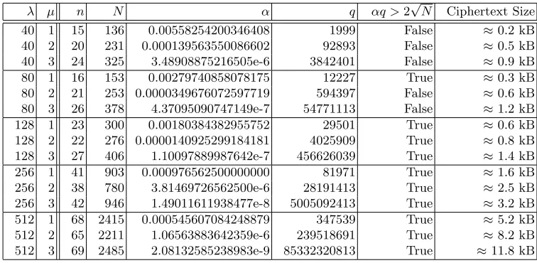
Our goal in the rest of the paper is to achieve full IND-CPA security for a symmetric Polly Cracker-type scheme down to the hardness of computing Gr¨obner bases. To this end, we introduce noisy variants of GB and IM in the next section. These variants ensure that the conditions of Theorem 7 do not hold any more. In particular, the condition that ri = fimodI are known will
be no longer valid.
6 Gr¨obner Bases with Noise
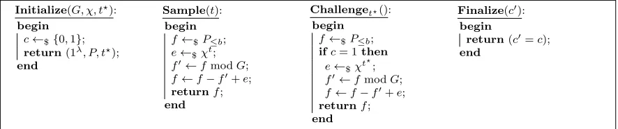
In this section, we introduce noisy variants of the problems presented in Section 3. The goal is to lift the restriction on the number of samples that the adversary can obtain and, following a similar design methodology to Polly Cracker, construct an IND-CPA-secure scheme. Put differently, we consider problems that naturally arise if we consider noisy encoding of messages inSPC. Similarly to [81, 74] we expect a problem which is efficiently solvable in the noise-free setting to be also hard in the noisy setting. We will justify this assumption in Section 6.1 by arguing that our construction can be seen as a generalisation of [81, 74].
The games below will be parameterised by a noise distributionχ. The discrete Gaussian distri-bution is of particular interest to us.
Definition 13 (Discrete Gaussian distribution). Let α >0 be a real number and q ∈N. The discrete Gaussian distribution χα,q, is a Gaussian distribution rounded to the nearest integer and reduced modulo q with mean zero and standard deviationαq.
In what follows we assume thatχ is defined over Q, i.e., ford >1 we have that χis a multidi-mensional noise distribution. For example, χ may simply consist of |S(I)≤b|independent discrete
Gaussian distributions, one for each m ∈ S(I)≤b. However, as pointed out in [66] simply using
the same Gaussian on each monomial is possibly not the best choice. Another notable special case is q = 2. In this case, χα,2 is a Bernoulli distribution with just one parameter 0 < p < 1, the
probability that 1 is returned.
We now define a noisy variant of the Gr¨obner basis problem. The task here is still to compute a Gr¨obner basis for some ideal I. However, we are now only given access to a noisy sample oracle which provides polynomials which are not necessarily in I but rather are “close” approximations to elements of I. Here the term “close” is made precise using a noise distributionχon Q.
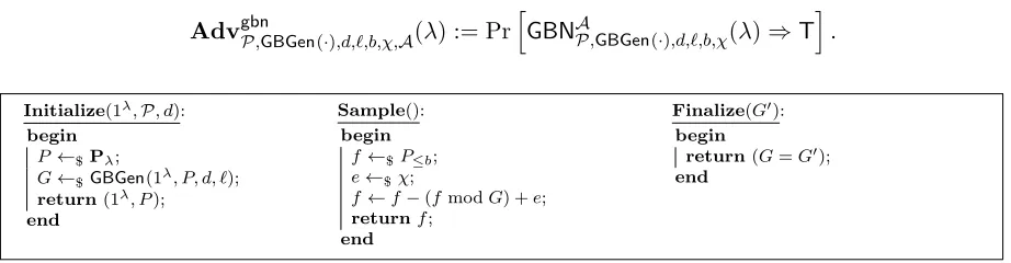
Definition 14 (The Gr¨obner basis with noise (GBN) problem). The Gr¨obner basis with noise problem is defined through game GBNP,GBGen(·),d,`,b,χ shown in Figure 5. The advantage of a PPT algorithm A in solving theGBN problem is
AdvgbnP,GBGen(·),d,`,b,χ,A(λ) := Pr
h
GBNAP,GBGen(·),d,`,b,χ(λ)⇒T
i .
Initialize(1λ,P, d): begin
P ←$Pλ;
G←$GBGen(1λ, P, d, `);
return(1λ, P);
end
Sample(): begin
f←$P≤b;
e←$χ;
f←f−(fmodG) +e; returnf;
end
Finalize(G0): begin
return(G=G0); end
Fig. 5.GameGBNP,GBGen(·),d,`,b,χ.
The essential difference between the noisy and noise-free versions of the Gr¨obner basis problem is that by adding noise we have eliminated the restriction on the adversary to call the Sample
oracle a bounded number of times. Put differently, ifχ is the delta distribution, theGBN problem degenerates to theGBproblem with an unbounded number of samples. Hence, in this case theGBN problem is easy. On the other hand if χ is uniform, theGBN problem is information-theoretically hard. Thus, the choice of χ greatly influences the hardness of the GBN problem. We leave the investigation of the noise parameter to future work.
As in the noise-free setting, we can ask various questions about the ideal I generated by G. One such example is solving the ideal membership problem with access to noisy samples fromI. In our definition the adversary wins the game if it can distinguish whether an element was sampled uniformly fromP≤b or from I≤b+χ.
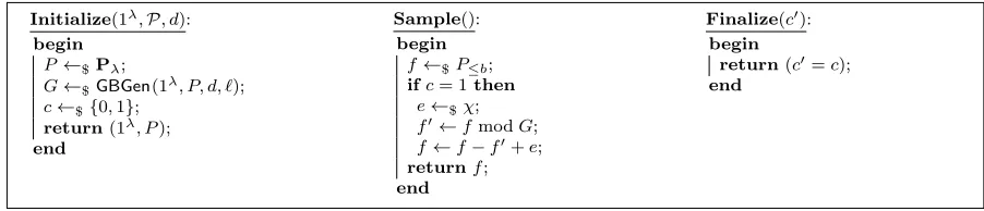
Definition 15 (The ideal membership with noise (IMN) problem). The ideal membership with noise problem is defined through game IMNP,GBGen(·),d,`,b,χ shown in Figure 6. The advantage of aPPT algorithmA in solving the IMN problem is defined by
AdvimnP,GBGen(·),d,`,b,χ,A(λ) := 2·PrhIMNAP,GBGen(·),d,`,b,χ(λ)⇒Ti−1.
Our definition of the IMN problem can be seen as an instantiation of Gentry’s ideal coset prob-lem [52] since both probprob-lems require distinguishing uniformly chosen eprob-lements in P≤b from those
inI≤b+χ.
Initialize(1λ,P, d):
begin P ←$Pλ;
G←$GBGen(1λ, P, d, `);
c←${0,1};
return(1λ, P);
end
Sample(): begin
f←$P≤b;
ifc= 1then e←$χ;
f0←fmodG; f←f−f0+e; returnf; end
Finalize(c0): begin
return(c0=c);
end
Fig. 6.GameIMNP,GBGen(·),d,`,b,χ. The adversary may callSamplemultiple times.
successful. On the other hand, aGBNoracle must recover coefficients of all monomial. For example, letG={x0+s0xn−1, . . . , xn−2+sn−2xn−1, x2n−1+sn−1xn−1}and henceS(I)≤b={xn−1,1}. Assume
the noise distributionχis such that the coefficient for xn−1 of the noise is uniform ∈Fq, while the
constant coefficient is always zero. For this shape and noise, it is easy to solve the IMN problem: any f ∈ P≤b with a nonzero constant coefficient is not an element of I =hGi. However, turning
this oracle into an adversary against theGBNproblem would require to recover allsi which are not even considered byIMN. Furthermore, the coefficients ofxn−1 are information-theoretically hidden,
so the distribution onI≤b+χ does not even depend on thesi (cf. [61]).
In fact, this type of counterexample is essentially the only thing that can go wrong: for a weaker variant of the IMN problem, which we aptly call the weakIMN problem (and define below in such a way to ensure that the adversary has to consider all monomials) we are able to show a reduction to theGBN problem. In this definition we lets:= dim(Q) =|S(I)≤b|, which is independent of the
randomness of GBGen(·). Given χ, we also define the distributions χt for t∈S(I)≤b by sampling
an element efrom Q according to χ and setting all but the coefficient corresponding to tto some independent uniform values.6 Hence, all coefficients except that corresponding totare information-theoretically blinded. Any algorithm which can distinguish samples followingI≤b+χtfrom uniform
samples inP≤b forall tcan be used to solve the GBN problem.
Definition 16 (The weak ideal membership with noise (WIMN) problem). The weak ideal membership with noise problem is defined through games WIMNG,χ,t? for t? ∈ S(I)≤b shown in
Figure 7. The advantage of a PPT algorithm A in solving theWIMN problem is defined by
AdvwimnP,GBGen(·),d,`,b,χ,A(λ) :=E
G h
min
t? 2·Pr
WIMNAG,χ,t?(λ)⇒T
−1
i ,
where the expectation is taken over Gsampled from GBGen(1λ, P, d, `).
Our definition of advantage is somewhat non-standard but it bears similarities to game defi-nitions in recent work on multi-instance security [17]. Indeed, we require that only those WIMN adversaries win the overall game which work for all t? ∈S(I)≤b for a particular Gr¨obner basis G.
As we shall see, only such adversaries allow us to recover the full Gr¨obner basis. Also, we note that the term “weak” is justified by the relation between WIMN and IMN. It is easy to see that if the IMN problem is hard, then so is the WIMN problem, while, as we have seen, the converse is not necessarily true. Finally, if d= 1 the IMN and WIMN problems are equivalent. We answer queries
6
Since the noise distributionχonly enters our construction viaχt, this has the side effect of removing all dependencies between the coefficients. In particular, we may as well assume thatχsamples the coefficients of all monomialst