Machine Learning for Stock Prediction Based on Fundamental Analysis

(1)

Scholarship@Western

Electronic Thesis and Dissertation Repository

4-23-2019 3:00 PM

Machine Learning for Stock Prediction Based on Fundamental

Analysis

Yuxuan Huang

The University of Western Ontario

Supervisor Capretz Luiz F.

The University of Western Ontario Co-Supervisor Ho Danny

NFA Estimation Inc.

Graduate Program in Electrical and Computer Engineering

A thesis submitted in partial fulfillment of the requirements for the degree in Master of Engineering Science

Follow this and additional works at: https://ir.lib.uwo.ca/etd

Part of the Artificial Intelligence and Robotics Commons

Recommended Citation Recommended Citation

Huang, Yuxuan, "Machine Learning for Stock Prediction Based on Fundamental Analysis" (2019). Electronic Thesis and Dissertation Repository. 6148.

https://ir.lib.uwo.ca/etd/6148

This Dissertation/Thesis is brought to you for free and open access by Scholarship@Western. It has been accepted for inclusion in Electronic Thesis and Dissertation Repository by an authorized administrator of

(2)

i

Abstract

Application of machine learning for stock prediction is attracting a lot of attention in

recent years. A large amount of research has been conducted in this area and multiple

existing results have shown that machine learning methods could be successfully used

toward stock predicting using stocks’ historical data. Most of these existing approaches

have focused on short term prediction using stocks’ historical price and technical

indicators. In this thesis, we prepared 22 years’ worth of stock quarterly financial data

and investigated three machine learning algorithms: Feed-forward Neural Network

(FNN), Random Forest (RF) and Adaptive Neural Fuzzy Inference System (ANFIS) for

stock prediction based on fundamental analysis. In addition, we applied RF based feature

selection and bootstrap aggregation in order to improve model performance and

aggregate predictions from different models. Our results show that RF model achieves

the best prediction results, and feature selection is able to improve test performance of

FNN and ANFIS. Moreover, the aggregated model outperforms all baseline models as

well as the benchmark DJIA index by an acceptable margin for the test period. Our

findings demonstrate that machine learning models could be used to aid fundamental

analysts with decision making regarding to stock investment.

Keywords: Stock prediction, fundamental analysis, machine learning, feed-forward

(3)

ii

Acknowledgments

I would like to thank my supervisor Dr. Luiz Fernando Capretz and co-supervisor Mr.

Danny Ho, for supporting me during my research here at Western University. The

patience, freedom and guidance they have provided me with are crucial to my personal

development at Western and the completion of this thesis.

I would also like to thank Tamer and Mohammed for their encouragement and advices

during this time.

Finally, I am also grateful to my parents and Brandy for their constant support throughout

my research and thesis writing. The delicious food and comfortable bed on my trips home

(4)

iii

List of Tables

Table 4.1: Dataset features after data preparation ... 29

Table 6.1: FNN hyperparameters ... 38

Table 6.2: FNN results for “Buy” portfolios ... 40

Table 6.3: FNN results for “Sell” portfolios ... 40

Table 6.4: ANFIS results for “Buy” portfolios ... 42

Table 6.5: ANFIS results for “Sell” portfolios ... 43

Table 6.6: RF hyperparameters ... 43

Table 6.7: RF results for “Buy” portfolios ... 45

Table 6.8: RF results for “Sell” portfolios ... 45

Table 6.9: Baseline model results for “Top20 Buy” portfolios ... 46

Table 6.10: Baseline model results for “Bottom20 Sell” portfolios ... 46

Table 6.11: Top six features selected by RF ... 48

Table 6.12: Results for “Top20 Buy” portfolio with selected features ... 49

Table 6.13: Results for “Bottom20 Sell” portfolio with selected features ... 49

Table 6.14: Results for “Buy” portfolios ... 52

(8)

vii

List of Figures

Figure 2.1: Real quarterly price of IBM stock(top) and random walk results of the same

length(bottom)... 8

Figure 2.2: FNN architecture ... 9

Figure 2.3: A small decision tree ... 11

Figure 2.4: Structure of an ANFIS ... 13

Figure 4.1: Historical quarterly revenue for BA – the original data ... 27

Figure 4.2: Historical revenue percentage change for BA ... 27

Figure 5.1: Data partition strategy ... 31

Figure 6.1: Relative return of FNN “Buy” portfolios for test quarters ... 39

Figure 6.2: Relative return of FNN “Sell” portfolios for test quarters ... 39

Figure 6.3: Relative return of ANFIS “Buy” portfolios for test quarters ... 41

Figure 6.4: Relative return of ANFIS “Sell” portfolios for test quarters ... 42

Figure 6.5: Relative return of RF “Buy” portfolios for test quarters ... 44

Figure 6.6: Relative return of RF “Sell” portfolios for test quarters ... 44

Figure 6.7: Feature importance based on RF ... 48

Figure 6.8: Relative return of aggregated “Buy” portfolios ... 51

(9)

viii

List of Appendices

(10)

Chapter 1

1 Introduction

1.1 Purpose

The main motivation for predicting changes in stock price is the potential monetary

returns. A large amount of research has been conducted in the field of stock performance

prediction since the birth of this investment instrument, as investors naturally would like

to invest in stocks which they have predicted will outperform the others in order to

generate profit by selling them later. A large inventory of stock prediction techniques has

been developed over the years, although the consistency of the actual prediction

performance of most of these techniques is still debatable. The techniques for stock

prediction can be classified into a small number of categories:

1. Fundamental analysis, where the predictions are made by studying the underlying

companies through their published financial statements.

2. Technical analysis, where the predictions are made by analyzing only the

historical prices and volumes.

3. Sentiment analysis, where the predictions are made by analyzing the published

articles, reports and commentaries pertaining to certain stocks.

The last category is much newer than the other two, as it is only made possible by the

(11)

general categories of stock prediction techniques, technical analysis and sentiment

analysis are primarily used for short-term prediction on the scale of days or less.

Fundamental analysis on the other hand, is used for mid-term and long-term prediction on

the scale of quarters and years [1]. In recent years, the popularity of applying various

machine learning and data mining techniques to stock prediction has been growing. The

majority of the existing studies using machine learning and data mining focus on creating

prediction models based on technical analysis and sentiment analysis [2] [3] [4]. Results

from many of these studies have shown that prediction models trained with historical

price and volume data can be successfully used towards short-term predicting [3] [4].

However, there is one major drawback for short-term prediction and high frequency

trading, which is frictional cost or trading commission. For an investor trading stocks

through a broker, there is typically a commission paid to the broker for each buy and sell.

The rate of commission varies from broker to broker, but it can really eat up the potential

profit as the trading frequency increases [5], even with discount brokers. Since the

short-term prediction models from many of the studies do not incorporate frictional cost in

evaluation [3] [4], the conclusiveness of the studies may be affected.

In this thesis, we aim to evaluate machine learning methods for long-term stock

prediction based on fundamental analysis. We do so by comparing the prediction

performance of three advanced machine learning methods based on fundamental analysis

using fundamental features. To develop and test the machine learning models, we used

data extracted from the quarterly financial reports of 70 stocks that appeared in the S&P

100 between 1996 and 2017. In order to evaluate the performance of different machine

learning methods, we rank the 70 stocks based on their predicted relative return.

Portfolios are constructed based on the ranking and the actual relative returns of the

portfolios are used as the evaluating criteria.

1.2 Contributions

In this thesis, we evaluated advanced machine learning methods for long-term stock

prediction based on fundamental analysis. We also proposed a portfolio selection method

(12)

predictors. For experimentation, we worked with real financial data extracted from

companies’ quarterly financial reports.

The main contributions of this thesis can be summarized as follows:

1. We organized and cleaned financial data extracted from 70 companies’ quarterly

financial reports across a period of 22 years.

2. We examined three machine learning algorithms for stock prediction based on

fundamental analysis: Adaptive Neural Fuzzy Inference System (ANFIS),

Feed-Forward Neural Network (FNN) and Random Forest (RF). A ranking based

portfolio selection method was used to construct portfolios based on predictions.

The relative returns of constructed portfolios were evaluated with respect to

benchmark index.

3. We used RF based feature selection method for identifying important features and

improving model performance.

4. We used bootstrap aggregating to assemble the prediction results from three

machine learning algorithms in order to improve the return of the constructed

portfolios.

1.3 Thesis Outline

The reminder of this thesis is organized as follows: In Chapter 2, the background

knowledge in stock prediction, financial analysis and related challenges is covered. The

introduction to the three machine learning methods used in this research is also included

in this chapter. In Chapter 3, researches in the area of the application of machine learning

methods in stock prediction are reviewed. Chapter 4 discusses the data set used in the

experiment as well as the details about the data preparation process. In Chapter 5, the

methodology of the proposed experiment is discussed in detail. The results we obtained

are presented and discussed in Chapter 6. Finally, the conclusion of the research and

(13)

Chapter 2

2 Background

2.1 Stock Prediction Basics

The purpose of this thesis is to apply supervised learning methods to the financial data of

particular stocks in order to predict future performance. A stock prediction problem like

this involves employing knowledge from both machine learning and the stock market.

Because of the cross-disciplinary nature of our research problem, it is necessary to cover

the important general concepts of stock prediction and financial analysis before

continuing.

2.1.1 Important Terms

As this thesis approaches the stock prediction problem from a software engineering

perspective, some knowledge of the terminologies from the finance domain is essential.

In order for clear understanding of the contents of this thesis, some important terms

which would be used later are defined here.

Universe of Stocks: The goal of this research is to build stock prediction models

to predict a set of stocks, and then select stocks from the set to construct portfolios. The

set of stocks is formally called a universe [6]. In this research, the universe of stocks

(14)

Absolute Return: Absolute return is the return an asset achieves over a certain

period of time, expressed as a percentage. The return is not compared to any other

measure or benchmark [7]. For example, assume you invest $100 into a stock A at time

t=0. You sell the investment at t=1 for $120. Then the absolute return of this investment

over the period of time between t=0 and t=1 is (120-100)/100 = 20%.

Relative Return: In contrast to absolute return, relative return is the return an

asset achieves over a period of time compared to the return of a benchmark over the same

period of time. The relative return is the difference between the absolute return of the

asset and the absolute return of the benchmark [8]. For example, assume you invest $100

into a stock A at time t=0. You sell the investment at t=1 for $120 to achieve an absolute

return of 20% from this investment. Over the same period of time from t=0 to t=1, the

benchmark S&P500 index achieves absolute return of 30%. Thus, the relative return of

your investment with respect to benchmark S&P500 is 20%-30% = -10% between t=0

and t=1. Note here that the relative return of your investment with respect to benchmark

is negative, even though it achieved positive absolute return. This means that you would

be better off investing into the S&P500 index fund, which exposes your investment to

much less risk than an individual stock does, for that period of time.

Portfolio: A portfolio is any combination of financial assets constructed and held

with the intention of earning a profit.

Equal Weight: Equal weight is a strategy used for constructing a portfolio or

index. In an equal-weight portfolio of stocks, each stock receives the equal weight, and

thus the same amount of investment.

Backtesting: In order to evaluate the performance of a stock investment strategy,

one can test the strategy in the real world by making a real or hypothetical investment

according to the strategy. The future return of the investment could validate the strategy.

This testing method is called forward testing. One obvious disadvantage of forward

testing is that it requires an extended period of testing time. Alternatively, a stock

investment strategy can be tested by simulating its usage on historical stock prices, where

(15)

testing method is called backtesting. Backtesting relies on the fundamental assumption

that a strategy which worked well in the past is likely to work well in the future. In other

words, history tends to repeat itself [9].

2.1.2 Types of Financial Analysis

There are various established techniques investors traditionally use for helping with

evaluating stocks and predicting future price movement. These techniques can be

classified into three major types: technical analysis, fundamental analysis and sentiment

analysis.

Technical Analysis: technical analysts evaluate investments and identify buying

or selling opportunities by analyzing statistical trends gathered from historical price and

volume. Unlike fundamental analysts, who attempts to evaluate a stock’s intrinsic value

using publicly available information, technical analysts assume that a stock’s price

already reflects all publicly available information. There are three premises that technical

analysis is based upon [10]:

1. Market action discounts everything

2. Prices move in trends

3. History repeats itself

Fundamental Analysis: fundamental analysis attempts to measure the intrinsic

value of a stock by considering a broad number of factors from the overall economy in

relation to industry performance and a company’s financial factors such as earnings,

profit margin, assets, liabilities and so on. Price movement history and volume are rather

insignificant to fundamental analysts. World famous investor Warren Buffet is well

recognized as a practitioner of fundamental analysis.

Sentiment Analysis: Sentiment analysis uses natural language processing and

text analysis to systematically extract and identify subjective information. Sentiment

analysis is widely applied to different areas. For stock market, sentiment analysis is used

(16)

market. Sentiment analysis is not within the scope of this research, thus it will not be

discussed in detail.

In general, fundamental analysis and technical analysis have different importance when

examined under the factor of the predicting horizon. Fundamental analysis is usually

preferred when the predicting time horizon is a quarter, a year or longer. Technical

analysis is preferred for short-term prediction such as for days or less.

2.1.3 Challenges of Stock Prediction

Stock trading is a process of buying and selling shares of publicly listed companies on a

stock exchange platform, with millions of investors and traders from all over the world

actively involved at any given time when the market is open. Stock market prediction is

an extremely complex and difficult problem because there are simply too many factors

and noises affecting the movement of the price. Many existing studies associated with

stock market prediction support the well-known Efficient Market H(EMH) [11],

according to which the price of a stock at any given time reflects all information available

about it and is therefore impossible to predict [12]. In Figure 2.1, we can compare the real

IBM historical price with randomly generated random walk results. One could easily be

led to believe that both price trends are generated randomly. There are three forms of

EMH, based on the degree of stock market efficiency:

Weak form EMH implies that the market efficiently reflects all past market

information. The hypothesis assumes that past rates of return have no effect on future

rates.

Semi-strong form EMH implies that the market efficiently reflects all publicly

available information. This hypothesis assumes that the stock price adjusts quickly to

absorb new information, e.g. a company’s financial reports. Semi-strong form

incorporates weak form EMH.

Strong form EMH implies that the market efficiently reflects all information,

(17)

achieve above average returns even if he/she was given new information that is not

available publicly. Strong form EMH incorporates weak form and semi-strong form

EMH.

Recent studies which have explored using machine learning and soft computing

techniques for stock prediction, have achieved results that challenge the weak and

semi-strong form EMH [17]-[23]. However, most of these studies use historical price,

technical indicators or investor sentiments as independent variables for model training

and prediction. The main motivation of our research is to develop machine learning

models to simulate the decision-making process of investment experts based on a stock’s

fundamental financial ratios.

Figure 2.1: Real quarterly price of IBM stock(top) and random walk results

(18)

2.2 Machine Learning Methods

This section presents background information on the machine learning methods used in

this thesis: FNN, RF, ANFIS. Because of the nature of our problem and dataset, all three

methods used are supervised learning methods.

2.2.1 Feed-forward Neural Network

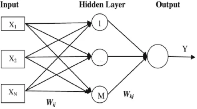
Feed-forward Neural Network (FNN), or Multi-Layer Perceptrons (MLP), is the simplest

and very versatile form of neural network architecture. An FNN consists of at least three

layers: an input layer, a hidden layer and an output layer. The architecture of a typical

FNN with one hidden layer is illustrated in Figure 2.2. The supervised learning technique

of gradient descent is used for backpropagation. In the training process, the change of

cost with respect to the weight between two nodes is calculated as [13]:

𝛥𝑤

_𝑗𝑖

(𝑛) = −𝛾

𝛿𝜀(𝑛)

𝛿𝑤_𝑗𝑖(𝑛)

(2.1)

where 𝛾 is the learning rate, 𝜀 is the error in the final output, 𝑤𝑗𝑖 is the weight between

neuron j and neuron i.

(19)

There are many hyperparameters that can be tuned during the model validation of an

FNN in order to achieve the optimal model generalization.

Weight Initialization Methods: The weights connecting neurons between

different layers must be initialized before training the model. Good choice of

initialization method could speed up the learning process of the network. Some of the

popular weight initialization methods include initializing weights to random small values

with normal distribution or uniform distribution.

Learning Rate: The learning rate controls the rate of adjustment to be made to

the weights with respect to the loss gradient. Traditionally, constant learning rate or

learning rate schedules are used. Common learning rate schedules include time-based

decay, step decay and exponential decay. In recent years, many established adaptive

learning rate methods such as Adagrad, Adadelta, RMSprop and Adam have become

popular.

Number of Hidden Layers: The number of hidden layers needs to be determined

during the initial design of any FNN. Generally, the number of hidden layers is based on

the size and dimension of the dataset. Deep neural networks with many hidden layers are

suitable for large datasets with high feature dimension.

Number of Hidden Units: The number of neurons in each hidden layer needs to

be determined as well. Just like the number of hidden layers, the number of hidden units

is also based on the size and dimension of the dataset.

Activation Functions: Each node in a neural network is a neuron that uses a

nonlinear activation function, except for the input neurons. For a regression problem, the

activation function of Rectified Linear Unit (ReLU) is typically used for hidden units.

2.2.2 Random Forest

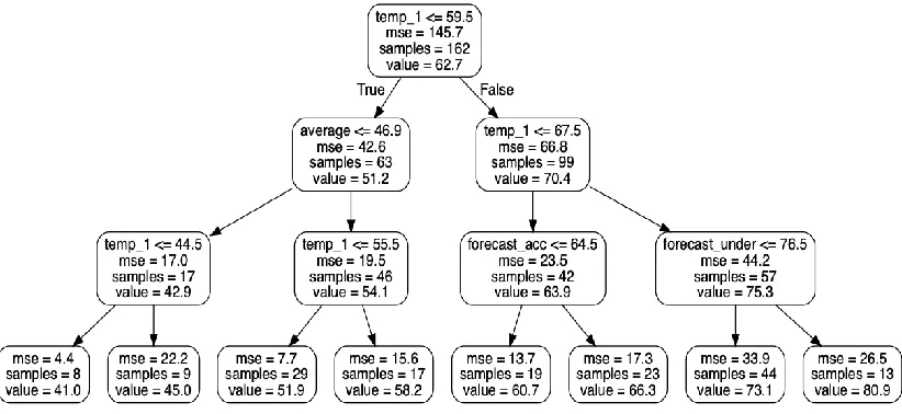
Random Forest (RF) is a flexible supervised learning algorithm which can be used for

both classification and regression tasks. It builds multiple decision trees during the data

(20)

RF takes the mean value of the output of all decision trees for a regression problem. For

classification problems, the majority voting from the decision trees is used as the result.

Many hyperparameters can be tuned to increase the performance of RF. A few of the

most important hyperparameters for RF are listed below:

Number of Estimators: This is just the number of decision trees the algorithm

builds before taking the maximum voting or the average of predictions. In general, a

larger number of decision trees increases the performance of the algorithm at the cost of

slower computation.

Minimum Sample Split: The minimum number of samples required to split an

internal node. This should be based on the size of the dataset.

Maximum Features: The number of features to consider when looking for the

best split. The dimension of the dataset needs to be taken into account when tuning this

hyperparameter.

(21)

2.2.3 Adaptive Neural Fuzzy Inference System

ANFIS is an instance of the more generic form of the Takagi-Sugeno-Kang (TSK) fuzzy

inference system. It replaces the fuzzy sets in the implication with a first order

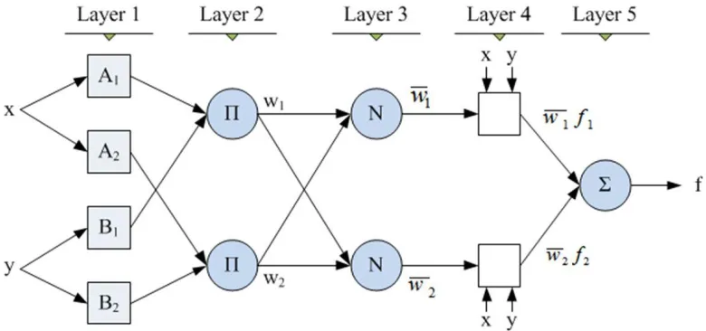
polynomial equation of the input variables [14]. The ANFIS system consists of rules in

IF-THEN form. In general, there are five different layers in an ANFIS system. Layer 1

converts each input value to the outputs of its membership functions:

𝑂

_𝑖𝑖

= 𝜇

_𝐴_𝑖

(𝑥) (2.2)

where 𝑥 is the input to node 𝑖 and 𝜇_𝐴_𝑖(𝑥) is the bell-shaped membership function with maximum equal to 1 and minimum equal to 0.

Layer 2 calculates the firing strength of a rule by simply multiplying the incoming

signals. Layer 3 normalizes the firing strengths:

𝑤

_𝑖

=

𝑤𝑖

∑ 𝑤_𝑗 _𝑗

(2.3)

Layer 4 consists of adaptive nodes with function defined as [14]:

𝑂

_𝑖4

= 𝑤

_𝑖

(𝑝

_𝑖

𝑥 + 𝑞

_𝑖

𝑦 + 𝑟

_𝑖

) (2.4)

where 𝑤_𝑖 is the normalized firing strength from the previous layer and (𝑝_𝑖𝑥 + 𝑞_𝑖𝑦 + 𝑟_𝑖) is a first order polynomial with three consequent parameters {𝑝𝑖, 𝑞𝑖, 𝑟𝑖} .

Layer 5 takes the weighted average of all incoming signals and delivers a final output:

𝑂

₁5

= 𝑜𝑣𝑒𝑟𝑎𝑙𝑙 𝑜𝑢𝑡𝑝𝑢𝑡 = ∑ 𝑤

_𝑖

𝑓

_𝑖

=

∑ 𝑤𝑖 𝑖𝑓𝑖

∑ 𝑤𝑖 𝑖

𝑖

(2.5)

Where 𝑓_𝑖 is the first order polynomial mentioned above. The structure of a typical ANFIS is shown in Figure 2.4.

Tuning an ANFIS involves determining the number of membership functions for each

input and the type of input membership function. For the MATLAB Fuzzy Toolbox

(22)

defining membership functions and fuzzy rules automatically based on the input data,

including grid partition, subtractive clustering and fuzzy C-Means clustering.

(23)

Chapter 3

3 Related Research

This section focuses on highlighting related studies for the application of machine

learning for stock prediction. We first look at researches that use classical approaches to

predict stock performance, specifically using fundamental analysis. Next, studies which

apply machine learning algorithms to stock’s technical data are examined. Finally, we

will cover approaches that use machine learning with fundamental analysis for stock

prediction. Thus, the related research covered in this section are increasingly similar to

ours.

3.1 Stock Prediction with Fundamental Analysis

As mentioned in the previous chapter, fundamental analysis techniques focus on

evaluating a stock’s intrinsic value based on publicly available financial ratios of the

company. The history of fundamental analysis may be traced back to the book “Security

Analysis” written by Benjamin Graham and David Dodd in 1934 [15]. This book laid the

intellectual foundation of what was later called value investing. Many researches have

been conducted in trying to formularize and extend the stock selection principles from the

book.

Piotroski [16] proposed a logistic regression model called F-Score for assessing strength

of a company’s financial position. F-Score was calculated based on nine financial criteria

(24)

profitability, liquidity and operating efficiency. Some of the financial ratios are defined as

follows:

𝑅𝑒𝑡𝑢𝑟𝑛 𝑜𝑛 𝐴𝑠𝑠𝑒𝑡𝑠(𝑅𝑂𝐴) =

𝑁𝑒𝑡 𝐼𝑛𝑐𝑜𝑚𝑒

𝑇𝑜𝑡𝑎𝑙 𝐴𝑠𝑠𝑒𝑡𝑠

(3.1)

𝐷𝑒𝑏𝑡 𝑅𝑎𝑡𝑖𝑜 =

𝑇𝑜𝑡𝑎𝑙 𝐷𝑒𝑏𝑡

𝑇𝑜𝑡𝑎𝑙 𝐴𝑠𝑠𝑒𝑡𝑠

(3.2)

𝐶𝑢𝑟𝑟𝑒𝑛𝑡 𝑅𝑎𝑡𝑖𝑜 =

𝐶𝑢𝑟𝑟𝑒𝑛𝑡 𝐷𝑒𝑏𝑡

𝐶𝑢𝑟𝑟𝑒𝑛𝑡 𝐴𝑠𝑠𝑒𝑡𝑠

(3.3)

𝐺𝑟𝑜𝑠𝑠 𝑀𝑎𝑟𝑔𝑖𝑛 =

𝑅𝑒𝑣𝑒𝑛𝑢𝑒−𝐶𝑜𝑠𝑡 𝑜𝑓 𝐺𝑜𝑜𝑑𝑠 𝑆𝑜𝑙𝑑

𝑅𝑒𝑣𝑒𝑛𝑢𝑒

(3.4)

𝐴𝑠𝑠𝑒𝑡 𝑇𝑢𝑟𝑛𝑜𝑣𝑒𝑟 𝑅𝑎𝑡𝑖𝑜 =

𝑇𝑜𝑡𝑎𝑙 𝑆𝑎𝑙𝑒𝑠

𝐴𝑣𝑒𝑟𝑎𝑔𝑒 𝑇𝑜𝑡𝑎𝑙 𝐴𝑠𝑠𝑒𝑡𝑠

(3.5)

Piotroski [16] backtested the F-Score model for stock selection with data from 1976 to

1996 and achieved positive results.

Similarly, Mohanram [17] developed a G-Score model for stock selection. The G-Score

model was calculated based on a different set of financial criteria extracted from a

company’s financial reports. These criteria are divided into three categories: Profitability,

Naïve Extrapolation and Accounting Conservatism. G-Score was backtested between

1978 and 2001, and a strong positive relationship was found between G-Score and

realized returns.

3.2 Stock Prediction with Machine Learning

3.2.1 Based on Technical Analysis

The majority of the existing studies that apply machine learning to stock prediction are

based on technical analysis [3] [4]. Machine learning models developed in these studies

(25)

popularity of technical analysis based models is due to the popularity of technical

analysis among the financial media and Wall Street financial advisors. In addition, stocks’

technical data are available in much larger volume compared with financial fundamental

data. This is because a stock’s price and technical indicators are available with a daily

sampling frequency, while its financial fundamental data is only published on a quarterly

basis.

Kimoto et al. [18] studied the use of feed-forward neural network for stock prediction

back in 1990. The inputs of their prediction model consisted of technical indicators as

well as some macroeconomic indices such as interest rate and foreign exchange rate.

They tested their model for generating buying and selling signals of the TOPIX index for

a 33 months period, from January 1987 to September 1989. The results show that the

neural network prediction model is able to achieve superior profit over the buy-and-hold

strategy.

Patel et al. [19] explored four different machine learning algorithms for stock price

predication, including Artificial Neural Network (ANN), Support Vector Machine (SVM),

Random Forest (RF) and naïve-Bayes. For input data, ten technical indicators were used.

They tested two approaches for model building. The first approach used the ten

continuous-valued technical indicators as is. The ten features were normalized before

being used for training. The second approach discretized the technical indicators to

represent the deterministic trend. For experiment, 10 years of daily historical data of two

stocks from S&P Bombay Stock Exchange (BSE) Sensex was used. The results indicate

that RF model outperforms the other three prediction models on overall performance. The

results also suggest that the prediction performance can be improved by converting inputs

from continuous-values data into discrete trend deterministic data. Patel et al. [20] also

proposed using a fusion of different machine learning techniques to improve prediction

performance. In the proposed two stage model, Support Vector Regression (SVR) was

first used to predict the value of technical indicators n days ahead. ANN, SVR and RF

were used in the second stage for predicting closing price n days ahead using predicted

technical indicators from the first stage. The results suggest that this two-stage fusion

(26)

Chong et al. [21] examined deep neural network for the stock prediction problem. The

assumption of this research was that properly tuned deep neural network is able to extract

features from a large set of raw data without relying on prior knowledge of predictors to

predict stock price movement with reasonable accuracy. For raw input data, 380

dimensional lagged stock price (38 stocks and 10 lagged prices) were used. Three

unsupervised methods were tested for feature extraction: principal component analysis

(PCA), autoencoder and restricted Boltzmann machine. As the research aimed to test

deep neural network for high frequency trading, the time interval between each

observation of stock price data was only 5 minutes apart. The deep neural network was

trained to predict stock price movement 5 minutes ahead. Standard root mean square

error (RMSE), mean absolute error (MAE) and normalized mean square error (NMSE)

were used for performance evaluation. The results show that the deep neural network

model achieves prediction performance similar to a simple linear autoregressive model.

Chong et al. [21] further experimented applying the deep neural network to the residuals

of the autoregressive model and achieved better results.

Bekiros et al. [22] compared ANFIS model and Recurrent neural network (RNN) model

for predicting the next day trend of NASDAQ and NIKKEI indices. For both models, the

previous closing price was used for predicting the next day’s closing price. To avoid data

snooping, they used data from 1971 to 1998 for model training and data from 1998 to

2002 for out-of-sample testing. The results suggest that the rate of return for ANFIS is

superior to that of the RNN model as well as the buy-and-hold strategy for both indices.

Atsalakis et al. [23] proposed an ANFIS model for predicting the next day price trend.

The proposed model took historical price and price moving average as inputs. Results of

the model are evaluated in terms of hit rate, which is defined as:

𝐻𝑖𝑡 𝑟𝑎𝑡𝑒 =

ℎ

𝑛

(3.6)

where ℎ denotes the number of correct predictions of the stock trend and 𝑛 denotes the

number of tests. Five stocks were chosen for backtesting. The ANFIS model achieved an

(27)

proposed model over the test horizon and compared it with the buy-and-hold strategy.

The ROR is defined as follows:

𝑅𝑂𝑅 =

𝑛𝑒𝑡 𝑔𝑎𝑖𝑛 𝑖𝑛 𝑠𝑡𝑜𝑐𝑘

𝑖𝑛𝑖𝑡𝑖𝑎𝑙 𝑖𝑛𝑣𝑒𝑠𝑡𝑚𝑒𝑛𝑡

(3.7)

The results suggest that the ANFIS model is able to achieve significantly higher ROR

than the buy-and-hold strategy for all five stocks. The ANFIS model was then compared

horizontally with neural network models from previous studies. Atsalakis claimed that

the proposed model is able to achieve a superior hit rate over previous models.

A k-NN based neuro-fuzzy system is proposed by Wei et al. [24]. In this study, the k-NN

method was used to select k instances of historical data that are most similar to the testing

input. These data were then used to create the predicting model. Thus, instead of using all

training data to train a model, k-NN was utilized to dynamically select k instances for

each prediction. The model was tested with TAIEX data from 1999 to 2004 and

compared with univariate neural network and fuzzy time series models. The results

suggest that the proposed model achieved a smaller RMSE than other baseline models.

3.2.2 Based on Fundamental Analysis

Next, we look at previous works on stock prediction and stock selection which combine

machine learning with fundamental analysis.

Quah and Srinivasan [25] developed a feed-forward neural network model for stock

selection using quarterly fundamental financial factors. Seven input features were chosen

as listed below:

𝐻𝑖𝑠𝑡𝑜𝑟𝑖𝑐𝑎𝑙 𝑃𝐸 𝑟𝑎𝑡𝑖𝑜 =

𝑃𝑟𝑖𝑐𝑒

𝐸𝑎𝑟𝑛𝑖𝑛𝑔 𝑝𝑒𝑟 𝑠ℎ𝑎𝑟𝑒(𝐸𝑃𝑆)

(3.8)

𝑃𝑟𝑜𝑠𝑝𝑒𝑐𝑡𝑖𝑣𝑒 𝑃𝐸 𝑟𝑎𝑡𝑖𝑜 =

𝑐𝑜𝑛𝑠𝑒𝑛𝑠𝑢𝑠 𝐸𝑃𝑆

(3.9)

(28)

𝐸𝑃𝑆 𝑢𝑛𝑐𝑒𝑟𝑡𝑎𝑖𝑛𝑡𝑦 = % 𝑑𝑒𝑣𝑖𝑎𝑡𝑖𝑜𝑛 𝑓𝑟𝑜𝑚 𝑚𝑒𝑑𝑖𝑎𝑛 𝐸𝑃𝑆 𝑒𝑠𝑡𝑖𝑚𝑎𝑡𝑒𝑠 (3.11)

𝑅𝑒𝑡𝑢𝑟𝑛 𝑜𝑛 𝐸𝑞𝑢𝑖𝑡𝑦(𝑅𝑂𝐸) =

𝑁𝑒𝑡 𝐼𝑛𝑐𝑜𝑚𝑒

𝑆ℎ𝑎𝑟𝑒ℎ𝑜𝑙𝑑𝑒𝑟 𝐸𝑞𝑢𝑖𝑡𝑦

(3.12)

𝐶𝑎𝑠ℎ𝑓𝑙𝑜𝑤 𝑌𝑖𝑒𝑙𝑑 =

𝑂𝑝𝑒𝑟𝑎𝑡𝑖𝑛𝑔 𝑐𝑎𝑠ℎ𝑓𝑙𝑜𝑤 (3.13)

The consensus EPS in Equation 3.9 is the average of financial analysts’ published

estimate EPS for next quarter. The last feature is a momentum factor derived by weighted

average of historical price appreciation. For the experiment, quarterly data of 25 stocks

from Q1 1993 to Q4 1996 were used. Note that there are only 16 observations for each

stock. The first 10 observations are used for training and last 6 observations for testing.

Due to the limited data size, another approach of moving window system is also tested.

The moving window system uses three quarters as a training sample and the subsequent

quarter as the testing sample. Stocks with the highest predicted returns were selected for a

portfolio for each of the test points. The absolute returns of the portfolios were evaluated.

The experimental results suggest that the proposed model is able to select portfolios that

outperform the market 10 out of 13 testing quarters and achieve superior returns.

However, as Quah and Srinivasan [25] noted in their conclusion, the experiment is

largely constrained by the availability of data. Thus, the conclusiveness of their results is

limited.

Lam [26] developed a similar feed-forward neural network model using more data. The

model is trained and tested on 364 S&P companies for the period from 1985 to 1995. The

inputs of the model included 16 financial statement variables and 11 macroeconomic

variables. Lam set up 4 experiments to test different combinations of predictors. The first

three experiments used one year’s, two years’ and three years’ financial data as inputs,

respectively. This setup helps to simulate the time series effect for analysis. The last

experiment combined three years’ financial data with macroeconomic data as inputs. Lam

did not separate part of the data set for model validation but instead presented results

(29)

stocks with the highest predicted returns were chosen to build a portfolio, and the

performance of the portfolio was evaluated. There are two key insights from the

experimental results. Firstly, the rate of return increases gradually from experiment 1

through 3. Such results show that integrating the technical analysis technique of

examining historical trend with fundamental analysis can improve the level of return.

Secondly, the results from experiment 4 suggest that the addition of macroeconomic

variables does not improve model performance.

Eakins and Stansell [27] examined whether using a neural network modelling procedure

for stock forecasting based on a set of financial ratios could improve investment returns.

They used the yearly financial data of all stocks listed on Compustat between 1975 and

1996. Stocks with small market capitalization or high volatility were filtered out. They

trained one model for each year using stocks’ financial ratios at the end of that year as predictors and next year’s real returns as independent variables. The top 50 stocks with

the highest predicted returns were selected into a portfolio for evaluation. Based on the

experimental results, they argue that the neural network selected portfolio is able to

consistently outperform the full sample as well as board market benchmarks, with an

average annual return of 17.1% over the 20-year test period. The full sample achieves an

average annual return of 7.93% while S&P 500 and Dow Jones Industrials achieve 11.4%

and 11.3% respectively over the same period.

Quah [28] compared three different machine learning models for stock selection based on

fundamental analysis. The machine learning methods tested in this research are FNN,

ANFIS and general growing and pruning radial basis function (GGAP-RBF). A dataset of

1630 stocks which were extracted within a period of ten years from 1995 to 2004 was

used. Out of the ten years’ annual data, only the last year’s data were used for test set.

Quah picked 11 of the most commonly used financial ratios as predictors based on

Graham’s book [15]. Instead of training the supervised learning models to do regression,

Quah converted the prediction problem into a classification problem by classifying target

variable into two classes. “Class 1” was defined as any stock which appreciates in share

price equal to or more than 80% within one year, otherwise was classified as “Class 2”.

(30)

appreciate over 80% within one year in any given year. Therefore, an over-sampling

technique was used on the minority class in order to balance the dataset. Over-sampling

was used on training set only for the purpose of avoiding data scooping. According to

the experimental results, both FNN and ANFIS models were able to achieve above

market average annual appreciation of selected stocks at 13% and 14.9% respectively.

The average annual appreciation of the market for the test set is 11.2%. On the other hand,

GGAP-RBF performed poorly. The author also mentioned in the conclusion that the

availability of financial data is a major limitation of this study.

Shen and Tzeng [29] combined soft computing model using the dominance-based rough

set approach (DRSA), formal concept analysis (FCA), and DEMATEL techniques for

exploring the usefulness of fundamental analysis. 17 financial ratios of 112 IT stocks

listed in Taiwan Stock Exchange from 2010 to 2013 were used for their research. Based

on their value appreciation over each period, the stocks are divided evenly into three

classes: “low”, “mid” and “high” holding-period-return (HPR). The DRSA was then

trained to classify stocks’ HPR based on their financial ratios. The test results suggest

that the DRSA model is able to separate winners and losers from the sample, as the

average predicted “high”, “low” and market benchmark index HPR over the test period

are 11.5%, -5.91% and 5.04% respectively. Moreover, FCA were conducted to extract the

six most important features as well as twenty decision rules. The six most important

features from FCA results are:

1. Revenue growth rate (REV)

2. Gross profit growth rate (GrossProfit) 3. ROA growth rate (ROA)

4. Debt ratio

5. Asset turnover rate

6. Average days for sales

(31)

𝐷𝐴𝑌𝑠 =

𝐴𝑣𝑒𝑟𝑎𝑔𝑒 𝑒𝑛𝑑𝑖𝑛𝑔 𝑖𝑛𝑣𝑒𝑛𝑡𝑜𝑟𝑦

𝑂𝑝𝑒𝑟𝑎𝑡𝑖𝑜𝑛𝑎𝑙 𝑐𝑜𝑠𝑡

× 365 𝑑𝑎𝑦𝑠 (3.14)

This study argues that the decision rules found could assist investors with investment

decisions.

Hargreaves and Hao [30] applied two decision tree based methods (CHAID & C5.0) and

FNN on stock trend prediction. Five financial ratios were used as predictors: Return on

Equity, Return on Assets, Analyst Opinion, Annual Growth and Price. The classification

models were used to predict positive of negative return in price for the next day. The

evaluation criteria used in this research are sensitivity and specificity defined as follows:

𝑆𝑒𝑛𝑠𝑖𝑡𝑖𝑣𝑖𝑡𝑦 =

𝑛𝑢𝑚𝑏𝑒𝑟 𝑜𝑓 𝑡𝑟𝑢𝑒 𝑝𝑜𝑠𝑖𝑡𝑖𝑣𝑒𝑠

𝑛𝑢𝑚𝑏𝑒𝑟 𝑜𝑓 𝑡𝑟𝑢𝑒 𝑝𝑜𝑠𝑖𝑡𝑖𝑣𝑒𝑠+𝑛𝑢𝑚𝑏𝑒𝑟 𝑜𝑓 𝑓𝑎𝑙𝑠𝑒 𝑛𝑒𝑔𝑎𝑡𝑖𝑣𝑒𝑠

(3.15)

𝑆𝑝𝑒𝑐𝑖𝑓𝑖𝑐𝑖𝑡𝑦 =

𝑛𝑢𝑚𝑏𝑒𝑟 𝑜𝑓 𝑡𝑟𝑢𝑒 𝑛𝑒𝑔𝑎𝑡𝑖𝑣𝑒𝑠

𝑛𝑢𝑚𝑏𝑒𝑟 𝑜𝑓 𝑡𝑟𝑢𝑒 𝑛𝑒𝑔𝑎𝑡𝑖𝑣𝑒𝑠+𝑛𝑢𝑚𝑏𝑒𝑟 𝑜𝑓 𝑓𝑎𝑙𝑠𝑒 𝑝𝑜𝑠𝑖𝑡𝑖𝑣𝑒𝑠

(3.16)

The results suggest that C5.0 decision tree achieved the best prediction sensitivity and

specificity, at the rate of 98% and 88% respectively.

A recent study by Namdari and Li [31] also used FNN on stock trend prediction. They

used 12 selected financial ratios of 578 technology companies on Nasdaq from 2012-06

to 2017-02 as their dataset. Instead of simply normalizing or standardizing these

continuous features, they discretized all features by conducting topology optimization.

For comparison, they also developed a different FNN model for predicting stock price

trend based solely on historical price for the same companies and the same period of

time. The results suggest that the FNN model based on fundamental analysis was able to

outperform the alternative model based on technical analysis with overall directional

accuracy of 64.38% and 62.84%, respectively.

Bohn [32] combined technical analysis, fundamental analysis and sentiment analysis and

compared a set of machine learning models for long-term stock prediction. He used a

(32)

experiment. Regression models were built, and ranks were induced based on the model

predictions for each validation and test week. He evaluated the model performance using

the Spearman rank correlation coefficient between predicted rank and actual rank. The

results suggest that the neural network model combined with iterative feature selection

could match the performance of a model developed with human expertise from an

investment firm.

Yu et al. [33] developed a novel sigmoid-based mixed discrete-continuous differential

evolution algorithm for stock performance prediction and ranking using stock’s technical

and fundamental data. The evaluation metrics and feature selection process used in this

study is the same as in [32]. 483 stocks listed in Shanghai A share market from Q1 2005

to Q4 2012 were used for model building and testing. The results suggest that proposed

(33)

Chapter 4

4 Data Preparation

One of the challenges we faced in this research was related to putting together a dataset

of stocks’ financial ratios for experimentation and testing. Building a dataset involves

gathering data from various sources and putting them together. Data also needs to be

prepared properly before being used for model training and testing. In the following

sections of this chapter, we will discuss how data samples are selected, compiled and

prepared.

4.1 Data Collection

Sample stocks used for this experiment were chosen from the S&P 100 Index

components. The index includes 102 leading U.S. stocks which represent about 51% of

the market capitalization of the entire U.S. equity market [34]. There are two major

reasons behind choosing the S&P 100 components as sample stocks. First, financial

fundamental ratios for the S&P 100 stocks are relatively complete and large in terms of

data volume. This is because these stocks are large-cap, and most of them were publicly

listed relatively early in history. Second, the S&P 100 components are well balanced

across different sectors, and we decided that the number of its components was suitable

for the size of our sample stock pool. Because the composition of the S&P 100 index is

(34)

Historical financial data for each of the S&P 100 components were retrieved online in csv

format [35]. The original dataset contains 40 features as illustrated in Appendix A. These

data were extracted from companies’ SEC 10_Q filings, which are published quarterly.

4.2 Filling Missing Data Values

The raw fundamental data retrieved from online for stocks in our universe have a

considerable fraction of data entries missing. According to Graham’s study on missing

data analysis [36], the existence of missing values in a dataset could create problems for

data handling, and thus ultimately generate invalid conclusions. For machine learning

problems in particular as most of machine learning methods are designed to have

complete data for training and testing missing values in the dataset must be handled

before being used for building machine learning models.

As covered in [36] [37], common approaches for dealing with missing data include:

1. Listwise deletion: Listwise deletion removes every record that has one or more

missing values. For data that is missing completely at random (MCAR), listwise

deletion would only lead to a decrease in statistical power. If the data is missing

not at random (MNAR), this approach may yield biased parameter estimates.

2. Pairwise deletion: Pairwise deletion is usually used in conjunction with a

correlation matrix. Each correlation is estimated based on the cases having data

for both variables. Thus, pairwise deletion maximizes all data available on an

analysis by analysis basis. As pairwise deletion also assumes that missing data are

MCAR, it can still yield biased parameter estimates if data is MNAR.

3. Mean substitution: This approach replaces missing values with the average of

the parameter values that are not missing. Use of the mean substitution may be

based on the fact that the mean is a reasonable guess of a value for a randomly

selected observation from a normal distribution. With missing values that are not

MCAR, the mean substitution could be a poor guess [37]. This approach can be

(35)

values with the average of values within defined subgroups in order to get better

estimations.

4. Maximum likelihood estimation (MLE): MLE uses available data to compute

maximum likelihood estimates using the maximum likelihood function. Again,

MLE also assumes that the data is at least missing at random (MAR), if not

MCAR.

Other methods not described above include dropping features and using expert

knowledge to manually fill in missing values. Dropping entire features may be a good

option if there are a large number of features and the density of missing values for a

feature is high. Filling in missing values manually with expert knowledge is only viable if

the number of missing values is small.

The original dataset has large blocks of missing values concentrated on a few features,

while other missing values sparsely populated across the entire dataset. We eventually

decided to use a combination of feature deletion and mean substitution. In cases where a

fundamental factor had large blocks of missing values or over 50% values missing, it was

removed. We also removed some non-fundamental features such as price high and price

low. After the feature dropping, there were still some sparsely located missing values

which account for less than 3% of total samples. These missing values were then

substituted by the average of the two adjacent values. For example, if the revenue data for

2015Q3 is missing, it is substituted by the mean of the revenue values of the 2015Q2 and

2015Q4.

4.3 Trend Stationary

Our target variable in this research is quarterly relative returns, while many features from

the raw dataset possess a clear global trend with respect to time. As we transfer this time

series problem into a supervised learning problem, these features with global trends could

hinder our machine learning models’ ability to generalize and provide reliable

predictions. We therefore took the percentage change between consecutive observations

(36)

∆𝑥

_𝑡

=

(𝑥𝑡−𝑥𝑡−1)

𝑥𝑡−1

× 100% (4.1)

An example of trend-stationarizing a feature is shown in Figure 4.1 and Figure 4.2.

Figure 4.1: Historical quarterly revenue for BA – the original data

(37)

4.4 Standardization

As the scales of features can vary dramatically, standardization was applied to all features

in order to improve the performance of our prediction models. Features are standardized

using the following formula:

𝑥

′

=

𝑥−𝑥̅

𝜎

(4.2)

Where 𝑥 is the original feature vector, 𝑥̅ is the mean of the feature vector, and 𝜎 is its

standard deviation.

4.5 Relative Return

In the experiment, a stock’s quarterly relative return with respect to the Dow Jones

Industrial Average (DJIA) was used as the target variable instead of simple absolute

return. The DJIA is one of the most widely used U.S. stock market benchmarks. The

relative return of a stock is the difference between its absolute return and the return of

some benchmark. There are two major benefits of using relative return instead of absolute

return in our experiment. First, by subtracting overall market performance from the

performance of each individual stock, we are able to filter out the factors affecting the

broader market. In theory, using such a technique helps to reduce the complexity of the

prediction problem and improve the prediction performance of our models. Second, it

saves the step of comparing with the benchmark again in evaluation.

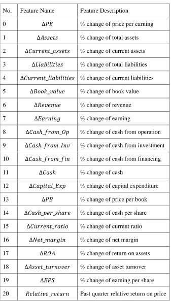
After the data preparation process was completed, we ended up with 21 features and 70

stocks. Each stock has 88 observations, ranging from Q1 1996 to Q4 2017, with an

interval of one quarter between two consecutive observations. The 21 features are

(38)

No. Feature Name Feature Description

0 ∆𝑃𝐸 % change of price per earning

1 ∆𝐴𝑠𝑠𝑒𝑡𝑠 % change of total assets

2 ∆𝐶𝑢𝑟𝑟𝑒𝑛𝑡_𝑎𝑠𝑠𝑒𝑡𝑠 % change of current assets

3 ∆𝐿𝑖𝑎𝑏𝑖𝑙𝑖𝑡𝑖𝑒𝑠 % change of total liabilities

4 ∆𝐶𝑢𝑟𝑟𝑒𝑛𝑡_𝑙𝑖𝑎𝑏𝑖𝑙𝑖𝑡𝑖𝑒𝑠 % change of current liabilities

5 ∆𝐵𝑜𝑜𝑘_𝑣𝑎𝑙𝑢𝑒 % change of book value

6 ∆𝑅𝑒𝑣𝑒𝑛𝑢𝑒 % change of revenue

7 ∆𝐸𝑎𝑟𝑛𝑖𝑛𝑔 % change of earning

8 ∆𝐶𝑎𝑠ℎ_𝑓𝑟𝑜𝑚_𝑂𝑝 % change of cash from operation

9 ∆𝐶𝑎𝑠ℎ_𝑓𝑟𝑜𝑚_𝐼𝑛𝑣 % change of cash from investment

10 ∆𝐶𝑎𝑠ℎ_𝑓𝑟𝑜𝑚_𝑓𝑖𝑛 % change of cash from financing

11 ∆𝐶𝑎𝑠ℎ % change of cash

12 ∆𝐶𝑎𝑝𝑖𝑡𝑎𝑙_𝐸𝑥𝑝 % change of capital expenditure

13 ∆𝑃𝐵 % change of price per book

14 ∆𝐶𝑎𝑠ℎ_𝑝𝑒𝑟_𝑠ℎ𝑎𝑟𝑒 % change of cash per share

15 ∆𝐶𝑢𝑟𝑟𝑒𝑛𝑡_𝑟𝑎𝑡𝑖𝑜 % change of current ratio

16 ∆𝑁𝑒𝑡_𝑚𝑎𝑟𝑔𝑖𝑛 % change of net margin

17 ∆𝑅𝑂𝐴 % change of return on assets

18 ∆𝐴𝑠𝑠𝑒𝑡_𝑡𝑢𝑟𝑛𝑜𝑣𝑒𝑟 % change of asset turnover

19 ∆𝐸𝑃𝑆 % change of earning per share

20 𝑅𝑒𝑙𝑎𝑡𝑖𝑣𝑒_𝑟𝑒𝑡𝑢𝑟𝑛 Past quarter relative return on price

(39)

Chapter 5

5 Methodology

In this chapter, we focus on discussing the details in the experiment process. Dataset

partition, evaluation metrics, feature selection and the final meta-algorithm for

aggregating results from different models are covered.

5.1 Dataset Partition

It is easy to overfit when building machine learning models for financial prediction

problems, especially with a limited amount of data. If all of the available data is used for

model training, the ability of the generalizability of the model to further unseen data

cannot be tested. Thus, it is crucial to hold-out part of the dataset as unseen data for

testing throughout the model training process. However, there are also various

hyperparameters which need to be tuned for optimal model performance. Different

machine learning methods have different hyperparameters, as discussed in chapter 2. If

we use the test dataset for model tuning, this would cause data snooping. As we already

know the tuned model performs well on test data, the test data is not really unseen, and

the generalizability of our machine learning model is weakened. Therefore, we

partitioned our dataset into three sets: training, validation and test. The training set

consists of 60% of the total data, while the validation set and test set consist of 20% each.

From a time series perspective, data from Q1 1995 to Q1 2008 is used for training; data

(40)

used for testing. Moreover, we train the models with the training set and the validation set

combined after model validation for generating the final test results on the test set. This

helps us to maximize the usage of data for training the models without data snooping.

Our strategy for data partition is illustrated in Figure 5.1.

Figure 5.1: Data partition strategy

5.1.1 Standardization

As discussed in the previous chapter, the dataset needs to be standardized before being

used for training. However, if standardization is applied before the data partition, we

essentially use all data for calculating the mean and standard deviation in Equation 4.2.

This means we use some information from the validation set and the test set even before

the model validation phase. Such practice could be problematic as it leads to data

snooping. On the other hand, standardizing data separately for training, validation and

test set can avoid data snooping, but this practice could lead to poor validation and test

results. This is because the mean and standard deviation of the same feature could be very

different among different partitions, while the model is only trained to generalize the

(41)

For our experiment, we first standardized the training set following Equation 4.2. Then

we used the mean and standard deviation from the training set to standardize the

validation set and the test set, following the formula:

𝑥

′

=

𝑥−𝑥̅̅̅𝑡

𝜎_𝑡 (5.1)

Where 𝑥̅_𝑡 and 𝜎_𝑡 are the mean and standard deviation of the feature in the training set. This practice helps to avoid data snooping without harming model performance.

5.2 Local Learning

We tried both building a single model for all stocks and building one model for each

stock. The two approaches can be classified as global learning and local learning. Models

trained with global learning enjoy a larger set of training data, while models trained with

local learning are more task specific and usually enjoy better performance [38]. Local

learning approach was proven to have better performance in our early experiment, and

thus we built one model for each stock for all three algorithms.

5.3 Evaluation Metrics

Previous studies on application of machine learning for stock prediction use different

metrics for performance evaluation, as discussed in Chapter 3. The metrics are selected

based on how the models are used for predicting stock performance:

Regression: For a regression model, the absolute or relative return of a stock at

some time in the future is estimated. Metrics such as root mean square error (RMSE),

mean square error (MSE), mean absolute error (MAE) and mean absolute percentage

error (MAPE) are usually used for evaluating the accuracy of the regression model.

Classification: For a classification model, the possible return of a stock is divided

into a small number of classes. For example, some studies [22] [23] which aim to predict

(42)

In this case, the hit rate defined as in Equation 3.6 is typically used. A stock’s future

return is classified more finely in some other studies [26] [28] [30]. In these cases, the

correlation between actual class and predicted class, or sensitivity and specificity defined

in Equation 3.15 and Equation 3.16 are usually used.

The goal of this project is to develop a system which can be used to guide stock portfolio

design strategy for long term investment. Therefore, simple and general evaluation

methods are preferred. We decided to build regression models to predict the price for

each stock, and then induce a ranking of the stocks by sorting their predicted relative

returns. The ranking can then be used for portfolio design, and the actual performance of

the portfolios in terms of real relative return can be evaluated with ease. The

performance evaluation methods of our model in training, validation and testing stages

are discussed separately in the following sections.

5.3.1 Training Loss

When training a regression model, the metric or the loss function depends on the specific

algorithm. Moreover, the loss function used in model training is also a hyperparameter

which can be tuned. For the FNN and ANFIS models, we use RMSE as the training loss

function. The RF algorithm, unlike FNN and ANFIS, does not involve training cycles and

loss function.

5.3.2 Validation Performance

After fitting a model with the training data, it is then evaluated on the validation data. The

stocks are ranked by their predicted relative returns for each of the quarters. The top one

third stocks with the highest ranking are selected into a portfolio. The real relative return

of the selected portfolio for each quarter is then calculated, assuming the portfolio is

equal weight. The average real relative return of the equal weight portfolio is calculated

with the formula:

𝑅

𝑝

̅̅̅̅

₌

1

#𝑞𝑢𝑎𝑟𝑡𝑒𝑟𝑠∑

𝑅

𝑝 #𝑞𝑢𝑎𝑟𝑡𝑒𝑟𝑠

Machine Learning for Stock Prediction Based on Fundamental Analysis

Scholarship@Western

Scholarship@Western

Machine Learning for Stock Prediction Based on Fundamental

Machine Learning for Stock Prediction Based on Fundamental

Analysis

Analysis

Abstract

Acknowledgments

Table of Contents

Table of Contents

List of Tables

List of Figures

List of Appendices

Chapter 1

1

Introduction

1.1

Purpose

1.2

Contributions

1.3

Thesis Outline

Chapter 2

2

Background

2.1

Stock Prediction Basics

2.1.1

Important Terms

2.1.2

Types of Financial Analysis

2.1.3

Challenges of Stock Prediction

Figure 2.1: Real quarterly price of IBM stock(top) and random walk results

2.2

Machine Learning Methods

2.2.1

Feed-forward Neural Network

𝛥𝑤

(𝑛) = −𝛾

(2.1)

2.2.2

Random Forest

2.2.3

Adaptive Neural Fuzzy Inference System

𝑂

= 𝜇

(𝑥) (2.2)

𝑤

=

(2.3)

𝑂

= 𝑤

(𝑝

𝑥 + 𝑞

𝑦 + 𝑟

) (2.4)

𝑂

= 𝑜𝑣𝑒𝑟𝑎𝑙𝑙 𝑜𝑢𝑡𝑝𝑢𝑡 = ∑ 𝑤

𝑓

=

(2.5)

Chapter 3

3

Related Research

3.1

Stock Prediction with Fundamental Analysis

𝑅𝑒𝑡𝑢𝑟𝑛 𝑜𝑛 𝐴𝑠𝑠𝑒𝑡𝑠(𝑅𝑂𝐴) =

(3.1)

𝐷𝑒𝑏𝑡 𝑅𝑎𝑡𝑖𝑜 =

(3.2)

𝐶𝑢𝑟𝑟𝑒𝑛𝑡 𝑅𝑎𝑡𝑖𝑜 =

(3.3)

𝐺𝑟𝑜𝑠𝑠 𝑀𝑎𝑟𝑔𝑖𝑛 =

(3.4)

𝐴𝑠𝑠𝑒𝑡 𝑇𝑢𝑟𝑛𝑜𝑣𝑒𝑟 𝑅𝑎𝑡𝑖𝑜 =

(3.5)

3.2

Stock Prediction with Machine Learning

₌