Available Online at www.ijcsmc.com
International Journal of Computer Science and Mobile Computing
A Monthly Journal of Computer Science and Information Technology
ISSN 2320–088X
IMPACT FACTOR: 5.258
IJCSMC, Vol. 5, Issue. 6, June 2016, pg.448 – 458
A Comparative Study of Load
Balancing Algorithms: A Review Paper
#1Zahra Mohammed Elngomi,
#2Khalid Khanfar
#1 PhD. Program in Computer Science, Sudan University of Science and Technology, Sudan
#2 Full professor Head of Information Security Department at Naif Arab University for Security, Saudi Arab
#1 Email: [email protected]
Abstract: A distributed system can be defined as a group of computing and communication resources shared by multiple users [1]. Load balancing is redistributing the workload among two or more computers so that more work gets done at the same time.
Load balancing is used to enhance the performance of system through a redistribution of load among processor or server machines. [1][2][3][5][7][8]
Load balancing is the concept of balancing load on servers using different types of load balancing techniques.
In this paper we describe different types of load balancing algorithms explaining their categories and classification compare different load balancing algorithms depending on specific qualitative parameters, review the performance analysis of diverse load balancing algorithms by using identified qualitative parameters.
In this paper, we consider into account two load balancing approaches static and dynamic.
Keywords: Distributed system, Load Balancing Algorithms, Dynamic Load Balancing, Static Load Balancing, Qualitative parameters
1.
Introduction
:In distributed systems used more than one processor to execute the program. Workload for a processor is the duration for processing time which takes to execute all processes assigned to that a processor. [2][8].
decide how to achieve a balance in the load distribution between processors so that the treatment processes is completed in the shortest possible time [2][7].
A server program has limited resources. These resources involve memory, hard disk, and processor speed, therefore server can be handle with certain number of clients. When the number of clients is increases a server will be overloaded and that may lead to slow down the performance, hang and crash issues. So, it is crucial to balance the load on a server and this can be achieved by keeping copies of servers and distribute the load among them [1][2][4].
Load balancing is very essential in distributed computing systems to improve the quality of service by dealing with changes in the load which occur over time which leads to enhance the performance of systems. The incoming requests are optimally distributed among available system resources to avoid resource bottlenecks as well as to better utilize available resources. Load balancing also provides horizontal scaling e.g., adding computing resources in order to address increased loads [1].
Load balancing increases availability, improves performance by increasing reliability, increases throughput, maintains, stability, optimizes resource utilization and provides fault tolerant capability. When the number of servers grows, the possibility of a failure is increasing and such failures must be handled carefully. The ability to maintain service without impact during any number of simultaneous failures is termed as high availability [1][8].
2.
Load balancing Problem in Distributed system:
An important issue in the distributed system environment is the performance which the response time of a request gets minimized.
When the demand of computing power increases, the load balancing problem becomes important. The problem of task scheduling and load balancing in distributed system are most important and challenging areas of research. [2]
The Problem here is to decide how to achieve a balance in the load distribution between processors so that the computation is completed in the shortest possible time. [2]
Load balancing is one of the most important problems in attaining high performance in distributed systems which may consist of many heterogeneous resources connected via one or more networks. In these distributed systems environment, it is possible for some computers to be heavily loaded while others are lightly loaded. This situation can lead to a poor system performance [3].
3.
Load Balancing Techniques and Algorithms:
Load balancing techniques are normally used for balancing the workload of distributed systems. Load balancing techniques are broadly classified into two types namely “Static load balancing” and “Dynamic load balancing”. The purpose of load balancing techniques, either static or dynamic, is to improve the performance by redistributing the workload among available server nodes [2].
Dynamic load balancing techniques react to the current system state, where as static load balancing techniques depends only on the average behavior of the system in order to balance the workload of the system transfer decisions are independent of the actual current system state. This makes dynamic techniques necessarily more complex than static one. But, dynamic load balancing policies have been believed to have better performance than static ones [1].
3.1 Types of load balancing algorithms:
Load balancing algorithms can be divided into three categories based on how the processes initiated:
Sender Initiated: In this type the load balancing algorithm is initialized by the sender. In this type of algorithm the heavily load node search for lightly load node to accept the load .The sender sends request messages and waits till it finds a receiver that can accept the load[2][3][5].
Receiver Initiated: In this type the load balancing algorithm is initiated by the receiver. This type of algorithm is the opiate of the above that the lightly load node search of a heavily node to get the load from it. The receiver sends request messages till it finds a sender that can get the load[2][3][5].
Symmetric: This type is a combination of both sender initiated and receiver initiated depending on the current state of the system[2][3][5].
3.2Approaches of Load balancing algorithms:-
Load balancing algorithm attempt to balance the load on whole system by migration the workload from heavily loaded nodes to lightly loaded nodes to enhance the system performances ,load balancing algorithms can classification into 2 categories as static and dynamic load balancing algorithms[2][3].
Most important tasks in load balancing are to determine load on each node, and then taking decision to migrate computing from one node to another.
Load balancer is essentially based on two characteristics. First, assign load to the best candidate node, and second, migration of load from heavily loaded node to lightly loaded node.
3.2.1 Static Load Balancing Approach
:Static load balancing mainly based on the information about the average of the system work load .It does not take the actual current system status into account [2][3] . The performance of processor is determined during the compilation time.
Static load balancing algorithms distribute load based on a fixed set of rules. These rules are related to load type, like processing power requirement, memory requirement, etc. [3].
The goal of static load balancing method is to reduce the execution time, minimizing the communication delays [2].
The main advantages of the static load balancing algorithms are that they minimize the execution time of the processes and they are simpler design and easy implementation. Also the major disadvantage of them is; they do not check load on other nodes. Hence, they cannot ensure whether balance is even or not. So they have lower performance [3].There are four types of static load balancing algorithms: -
3.2.1.1 Round Robin Algorithm:
3.2.1.2Randomized Algorithm:
Randomized algorithm choosiest he slave processors using random numbers. The slave processors are chosen randomly following random numbers generated depending on a statistic distribution. Randomized algorithm can obtain the best performance among all load balancing algorithms for particular special purpose applications [2][9].
3.2.1.3Central Manager Algorithm:
The Central Manager Algorithm uses central node as a coordinator to distribute the workload among the slave processors. The rule that is followed to choose the slave processor is to assign the job to the processor that have the least load. The central processor is able to gather all slave processors load information and take the decision of load balancing depending on this information so we expected a good performance when applying this algorithm. The main disadvantage of this type is the high degree of inter-process communication that could make a bottleneck state [2][9].
3.2.1.4Threshold Algorithm:
In this algorithm, the processes are assigned immediately to the server nodes upon creation [1][2] . Server nodes for new job are selected locally without sending remote messages. Each server node keeps a copy of the system's current load. The load of a processor can be characterized by one of the three levels: under loaded, medium, and overloaded. Two threshold parameters tunder and tupper can be used to describe these levels:
Under loaded - load <tunder Medium - tunder ≤ load ≤ tupper Overloaded - load >tupper
At first, all processor are assumed to be under-loaded. When the load of a processor changes, it sends a message to all other processors that are related with the new load state, updating them as to the actual current load state of the entire system. Each process gets allocated locally when the processor is under load , otherwise, a remote under-loaded processor is selected, and if no such host exists, the process is also allocated locally [1][2]
Thresholds algorithm have large number of local process allocations so it has low inter-process communication that decreases the overhead of the whole system which leads to improve the performance [1][2].
The main disadvantage of the threshold algorithm is that all processes are assigned locally when the processors are overhead. It does not take the execution time in consideration which impacts the performance of the entire system [2][10].
3.2.2Dynamic Load Balancing Approach:
Dynamic load balancing algorithms distribute the work load at run time. The decision of balancing the load is taken based on the current status of the system. The master node is able to collected the information of the slave processors and use this information to assign the process to the processor [1][2][3][7].
Dynamic load balancing can be done in two different ways: distributed and non-distributed. In the distributed one, the load balancing is made by all nodes in the system and the task of the load balancing is shared among them[2]. Also the interaction among nodes to achieve load balancing can be categories to: cooperative and non-cooperative. In a cooperative, the nodes work side-by-side to achieve load balancing. The objective is to improve the overall system performance. In a non-cooperative, each node works independently to achieve its own objectives. This improves the response time of a local task [2].
In distributed Dynamic load balancing algorithms, each node in the system communicates with every other node so it leads to a high degree of inter process communication. The advantage of this: it gives a good fault tolerance. Even if one or more nodes in the system fail, it will not impact the entire load balancing process. This can improve the performance.
into clusters, where each cluster is of a centralized form [2]. A central node in the cluster is chosen by using election technique. The load balancing of the system is executed by the central nodes. In all cluster centralized dynamic load balancing, fewer messages are generated rather than the semi distributed case. However, centralized algorithms can cause a bottleneck. Overall, the Dynamic Load Balancing is more complex than static but it has apriority rather than Static load balancing because it gives better performance than the static one [3].There are two types of dynamic load balancing:-
3.2.2.1 Central Queue Algorithm, Local Queue Algorithm:
In Central Queue Algorithm, the main host stores new task and unfulfilled requests in a cyclic FIFO queue. Each new task arriving at the queue manager gets inserted into the queue. Whenever a request for an activity is received by the queue manager, it removes the first activity from the queue and sends it to the requester. If the queue is empty then there are no ready activities in the queue. Thus, the request is buffered, until a new activity is available. When a new activity arrives, the queue manager checks the queue to see if there are unanswered requests in the queue, the first such request is removed from the queue and the new activity is assigned to it[10].
It works on the principle of receiver initiated. So when a processor load falls under the threshold, the local load manager sends a request for a new activity to the central load manager. The central load manager answers the request immediately if a ready activity is found in the process-request queue, or queues the request until a new activity arrives.[2][10]
3.2.2.2 Local Queue Algorithm
The main feature of Local Queue algorithm is the dynamic process migration support. The concept of the local queue algorithm is the processing of all new processes locally with process migration when the host load falls under threshold limit. This is a user-defined parameter. This parameter defines the minimal number of ready processes that the load manager attempts to provide on each processor [2]. In first step, new processes created on the main host are allocated on all under loaded hosts. The number of parallel activities created by the first parallel construct on the main host is usually sufficient for allocation on all remote hosts.
When the host gets under loaded, the local load manager attempts to get several processes from remote hosts. It randomly sends requests with the number of local ready processes to remote load managers. When a load manager receives such a request, it compares the local number of ready processes with the received number. If the former is greater than the latter, then some of the running processes are transferred to the requester and an affirmative confirmation with the number of processes transferred is returned [10].
3.2.3Dynamic load balancing control mechanism:
Dynamic load balancing can be classified into two different schemes: distributed and non-distributed. In a distributed scheme, all nodes work to gather to achieve the balance of load in the whole system, the interaction between nodes can take two forms cooperative and non-cooperative. In a cooperative form, all nodes have a common goal. They work together to achieve a global objective, e.g., to improve the system’s overall response time. In a non-cooperative form, each node tries to achieve its goals by working independently to improve a local task’s response time [3][7] .Cooperative form is stable but more complex and higher overhead communications while the non-cooperative form is instable but simple and less overhead communications [3].
In a distributed scheme, only one node or some nodes are responsible for load balancing in the system, non-distributed based dynamic load balancing can take two forms: centralized and semi non-distributed. In a centralized form, the load balancing algorithm is only executed by one node called central node. The central node is responsible for load balancing of the whole distributed system. Other nodes in the distributed system react with the central node but not with each other. In a semi-distributed form, nodes of the distributed system is split into groups, each group has central node responsible for load balancing in the group , Load balancing of the whole distributed system is achieved through the cooperation of the central nodes of each group.[7]
Centralized form generates fewer messages than the semi distributed form, but there is a possibility that this central node could cause a bottleneck which can cause crash of systems. Centralized form is suitable for small networks.[7]
3.2.4 Dynamic load balancing Model:
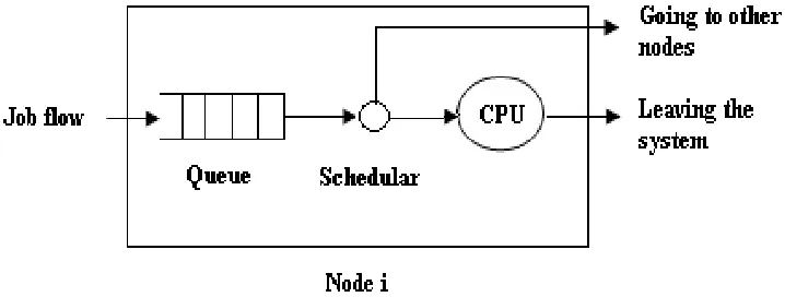
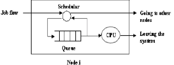
Load balancing algorithms model is consists of a scheduler, an infinite buffer and a processor. The scheduler is responsible of schedule the jobs arriving at the node so that the mean aim of it minimize response time for jobs . In the case there are not a scheduler in a node, the jobs is processed in three steps : firstly the a job insert into the buffer, secondly waits in the queue for processing, then send from the queue to the processor for processed and when the processing is finished it is leaves system.[1][11]
Though, in case the a scheduler is exist , three policies used to control the flow of processes depended on the place of a scheduler ,we can classify in to:
Queue Adjustment Policy (QAP) Rate Adjustment Policy (RAP)
Combination of Queue and Rate Adjustment Policy (QRAP).
3.2.4.1 Queue Adjustment Policy (QAP):
In this policy the scheduler is placed after the queue immediately. The objective of this algorithm is to try to balance the jobs in the queues of all nodes. When a job arrives at node i, the a scheduler checks the queue ,if it is empty, the job will be sent immediately to processor, If is not the job will be buffered in the queue.
The scheduler of node i is check the queue lengths of other nodes periodically that node i can communicate with. When an imbalance exists (some queues are too long than another queues), the scheduler will make a decision of how many jobs in the queue should be transferred and where each of the jobs should be sent to [1] [11][12].
3.2.4.2 Rate Adjustment Policy (RAP):
In this policy the scheduler is placed before the queue immediately. When a job arrives at node i, the scheduler makes a decision of where the job should be sent, whether it is to be sent to the queue of node i or to other nodes. If the job has inserted into the queue, it will be processed by processor and will not be transferred to other nodes[1][11][12]
Figure 1(b) Node model of rate adjustment policy
3.2.4.3
Hybrid Policy: Combination of Queue and Rate Adjustment Policy (QRAP):This policy is a combination of the two above policy, the scheduler is allowed to adjust the incoming job rate and also allowed to adjust the queue size of node i in some situations. Because we consider a dynamic situation, especially when we use RAP, in some cases, the queue size may exceed a predefined threshold and load imbalance may result. Once this happens, QAP starts to work and guarantees that the jobs in the queues are balanced in the entire system.[11]
Figure 1(c) Node model of combination of queue and rate adjustment policy.
4.
Qualitative Parameters:
There are multiple parameter which are used to measure the performance and qualitative of the static and dynamic algorithms. In this section we describe them:
4.1 Nature:
4.2 Overload Rejection:
This factor is needed when the load balancing is not possible. In this case, additional overload rejection measures are needed. These measures will stop when the overload situation end. Static load balancing algorithms does not support redistribution task when a task assigned to the processor so no relocation overhead, but Dynamic Load Balancing algorithms suffer more overhead relatively as relocation of tasks takes place [2].
4.3 Reliability:
This factor is related with the ability of algorithm to continuous in an excellent way when one or more machine fail. Dynamic load balancing is more reliable than the static because no task/process will be transferred to another host in case a machine fails at run-time in static.
4.4 Adaptability:
This factor is used to check whether the algorithm has ability to adapt with varying or changing situations. Static load balancing algorithms are not adaptive. Dynamic load balancing algorithms are adaptive [4][9].
4.5 Stability:
This is related with the delays in the transfer of information between processors and the benefits of the load balancing algorithm which leads to obtaining a faster performance.[2]
Static load balancing algorithm is more stable than the dynamic one because there is no information exchanging among processors during the run time [2][4][9].
4.6 Predictability:
This factor is related with the deterministic or nondeterministic factor that is to predict the outcome of the algorithm. Dynamic load balancing algorithm’s behavior is unpredictable because everything is done at run time. However Static load balancing algorithm is a predictable behavior as everything has been done at compilation-time [2] [9].
4.7 Cooperative:
This parameter gives that whether processors share information between them in making the process allocation decision or not during execution.
In a cooperative schemes, all processors work together to make the decisions. These are stable but more complex and cause overhead because they involve large communication. While in a non-cooperative schemes, etch processor work as autonomous processor and makes decisions independently of actions of other entities. These are instable but simple and involve less scheduling overhead [3][4].
4.8 Fault Tolerant:
4.9 Resource Utilization:
Static load balancing algorithms have less resource utilization as static load balancing methods just try to assign tasks to processors in order to achieve minimum response time ignoring the fact that the using of this task assignment may result into a situation in which some processors finish their work early and sit idle due to lack of work.
Dynamic load balancing algorithms have relatively better resource utilization as they take care of the fact that load should be equally distributed to processors so that no processors should sit idle [4].
4.10 Process Migration:
Process migration parameter provides a system with information so the system can decide to export a process or not. The process migration algorithm is capable to decide whether it should redistribute the load during the execution of the process or not [2].
4.11 Preemptiveness:
This factor is related with checking the fact that whether load balancing algorithms are inherently non-preemptive as no tasks are relocated .Dynamic load balancing algorithms are both non-preemptive and non-non-preemptive [2].
4.12 Response Time:
"How much time does a distributed system that uses a particular load balancing algorithm take to respond? " [2]
Dynamic load balancing algorithms take longer time than of the Static load balancing algorithms, because dynamic have take a time to make redistribute decision of the processes among the processors [2].
4.13 Waiting Time:
Waiting Time is the total of the times which a process spent in the waiting queues [2].
4.14 Turnaround Time:
Turnaround Time is the time between insert the process into the processor and the time of completion [2].
4.15 Through put:
Throughput is the quantity of data transferred successfully from place to another place in determined time [2].
4.16 Processor Thrashing:
5.
Conclusion:
Load balancing is required to distribute the workload evenly across all nodes to achieve high performance; with minimum overheads .There is no particular load balancing techniques fits for all distributed systems and we must choose the technique suitable to system architecture and requirements. If the system requires Stability we choose static load balancing regardless to performance issue or if the system requires higher performance we can be used dynamic load balancing technique.
Always the time dynamic load balancing techniques give better performance than static load balancing technique. Good load balancing algorithms depended on good task scheduling techniques. There are many parameters to measurement the efficiency of load balancing techniques such as response time, resource utilization, overhead associated, fault tolerant, centralized or decentralized, reliability, stability, adaptability, cooperative, process migration, scalability and throughput.
References:-1. Soundarabai .P ,Sahai .R , Venugopal .R, Patnaik .L : COMPARATIVE STUDY ON LOAD BALANCING TECHNIQUES IN DISTRIBUTED SYSTEMS, International Journal of Information Technology and Knowledge ManagementVolume 6, No. 1, pp. 53-60 , December 2012.
2. Abhijit A. Rajguru, S.S. Apte : A Comparative Performance Analysis of Load Balancing Algorithms in Distributed System using Qualitative Parameters, International Journal of Recent Technology and Engineering (IJRTE) ISSN: 2277-3878, Volume-1, Issue-3, August 2012 .
3. Rajani .SH, Garg .N: A Clustered Approach for Load Balancing in Distributed Systems, SSRG International Journal of Mobile Computing & Application (SSRG-IJMCA) – volume 2 Issue 1, Jan to Feb 2015.
4. Kanungo .P : MEASURING PERFORMANCE OF DYNAMIC LOAD BALANCING ALGORITHMS IN DISTRIBUTED COMPUTING APPLICATIONS, International Journal of Advanced Research in Computer and Communication Engineering Vol. 2, Issue 10, October 2013 .
5. Gupta .R , Ahmed .J: Dynamic Load Balancing By Scheduling In Computational Grid System, International Journal of Advanced Research in Computer Science and Software Engineering Volume 4, Issue 6 ISSN: 2277 128X, June 2014.
6. Razzaque .M , Hong. ch :Dynamic Load Balancing in Distributed System: An Efficient Approach, Department of Computer Engineering, Kyung Hee University , 1, Seocheon, Giheung, Yongin, Gyeonggi, Korea, 449-701. 7. Alakeel .A : A Guide to Dynamic Load Balancing in Distributed Computer
System ,IJCSNS International Journal of Computer Science and Network Security, VOL.10 No.6, June 2010. 8. Beniwal .R , Garg .A : A comparative study of static and dynamic Load Balancing Algorithms , International
9. Deepika, Wadhwa.D, Kumar.N: Performance Analysis of Load Balancing Algorithms in Distributed System, Advance in Electronic and Electric Engineering.
ISSN 2231-1297, Volume 4, Number 1 ,2014.
10. Sharma.S, Singh.S, Sharma.M: Performance Analysis of Load Balancing Algorithms, International Journal of Computer, Electrical, Automation, Control and Information Engineering Vol:2, No:2, 2008.
11. Naaz. S, Alam.A, Biswas.R :Load Balancing Algorithms for Peer to Peer and Client Server Distributed Environments,International Journal of Computer Applications (0975 – 888), Volume 47– No.8, June 2012