Differential Addition in generalized
Edwards Coordinates
Benjamin Justus and Daniel Loebenberger
Bonn-Aachen International Center for Information Technology Universit¨at Bonn
53113 Bonn Germany
Abstract. We use two parametrizations of points on elliptic curves in generalized Edwards form x2
+y2
= c2
(1 +dx2
y2
) that omit the x -coordinate. The first parametrization leads to a differential addition for-mula that can be computed using 6M+ 4S, a doubling formula using 1M+ 4Sand a tripling formula using 4M+ 7S. The second one yields a differential addition formula that can be computed using 5M+ 2S and a doubling formula using 5S. All formulas apply also for the case c 6= 1 and arbitrary curve parameterd. This generalizes formulas from the literature for the special casec = 1.
For both parametrizations the formula for recovering the missing X -coordinate is also provided.
Keywords. Elliptic curve, Edwards form, addition formula, differential addition
1
Introduction
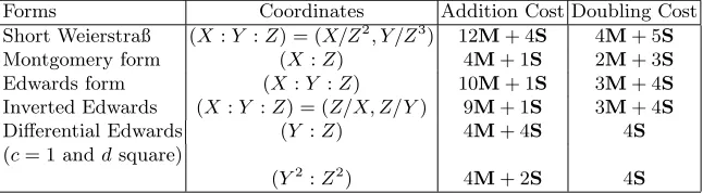
Efficient arithmetic (addition, doubling and scalar multiplication) on elliptic curves is the core requirement of elliptic curve cryptography. It is the corner-stone in applications such as the digital signature algorithm (DSA), see [10], and Lenstra’s elliptic curve factoring method [11]. Various ways of representing elliptic curves have been proposed for the purpose of efficient arithmetic. For an overview, the reader can consult the standard reference [7] or the online Explicit-Formulas Database (EFD)1. We have selected some of the top candidates and
summarized them in the table below. HereM(resp.S) refers to multiplication (resp. a squaring) in the field. We ignore in this paper multiplications by a con-stant and the additions in the field, since their cost is negligible when compared to the cost of multiplication or squaring.
With the advent of Edwards coordinates [8], extensive recent work [1–4] has provided formulas for addition on Edwards form that are more efficient (by a constant factor) than what is known for other representations. This makes the Edwards form particularly interesting for cryptographic applications.
1
Castryck, Galbraith and Farashahi [6] present doubling formulas for Edwards form withc= 1 like the one given in Corollary 1. They do not consider the case
c6= 1 and do not provide a general (differential) addition formula.
Gaudry and Lubicz [9] present general efficient algorithms for a much broader class of curves. In order to adapt their ideas to the context of elliptic curves in generalized Edwards form, one needs to explicitly express the group law in terms of Riemann’sϑfunctions. Due to our inability to do so, we derive in this work formulas for elliptic curves in generalized Edwards form directly. We are in good company here; Castryck, Galbraith and Farashahi write: “This is an euphemistic rephrasing of our ignorance about Gaudry and Lubicz’ result, which is somewhat hidden in a different framework.”
Special cases of our result can also be found on EFD: There are several formu-las given forc= 1 under the assumption that the curve parameterdis a square in the field. This restriction on the curve parameter dis annoying in practice, as the group law on elliptic curves in Edwards form is not complete anymore if
dis a square in the field. The formulas on EFD are on one hand consequences of [9] but can also be deduced from our general formulas in Theorem 1 and Corollary 1, as explained at the end of section 3.
Table 1.Some coordinate choices with fast arithmetic
Forms Coordinates Addition Cost Doubling Cost
Short Weierstraß (X:Y :Z) = (X/Z2
, Y /Z3
) 12M+ 4S 4M+ 5S
Montgomery form (X :Z) 4M+ 1S 2M+ 3S
Edwards form (X:Y :Z) 10M+ 1S 3M+ 4S
Inverted Edwards (X:Y :Z) = (Z/X, Z/Y) 9M+ 1S 3M+ 4S
Differential Edwards (Y :Z) 4M+ 4S 4S
(c= 1 anddsquare)
(Y2
:Z2
) 4M+ 2S 4S
In this work, we use two parametrizations for elliptic curves in generalized Edwards form to obtain efficient arithmetic: In the first parametrization a point on the curve is represented by the projective coordinate (Y :Z). Notice that the
The second parametrization also omits theX-coordinate. Additionally it uses the squares of the coordinates of the points only. On elliptic curves in generalized Edwards form, addition can be done with 5M+ 2Sand point doubling with 5S. We also provide a tripling formula for this second representation. For point doubling we get completely rid of multiplications and employ squarings in the ground field only. This is desirable since squarings can be done slightly faster than generic multiplications, see for example [7]. This second representation is best suited when employed in a scalar multiplication. Again we explicitly consider all formulas also for the casec 6= 1. On EFD several formulas for this parametrization can be found, but only for the special casec= 1 anddbeing a square in the ground field. The idea of this representation can already be found in Gaudry and Lubicz [9], section 6.2.
The plan of the paper is as follows. We recall the basics of Edwards coordi-nates in the next section and describe the addition, doubling and tripling formula in section 3. The formula for recovering theX-coordinate is given in section 4. The parametrization of the points that uses the squares of the coordinates only is analyzed in section 5.
2
Edwards Form
We describe now the basics of elliptic curves in generalized Edwards form. More details can be found for example in [3, 4]. Such curves are given by equations of the form
Ec,d: x2+y2=c2(1 +dx2y2),
where c, d are curve parameters in a field k of characteristic different from 2. Whenc, d6= 0 anddc4
6
= 1, the addition law is defined by
(x1, y1),(x2, y2)7→
x1y2+y1x2
c(1 +dx1x2y1y2)
, y1y2−x1x2 c(1−dx1x2y1y2)
. (1)
For this addition law, the point (0, c) is the neutral element. The inverse of a point P = (x, y) is −P = (−x, y). In particular, (0,−c) has order 2; (c,0) and (−c,0) are the points of order 4. When the curve parameterdis not a square in
k, then the addition law (1) is complete (i.e. defined for all inputs).
3
Representing Points in Edwards Form
As explained in the introduction, we represent a pointP on the curveEc,dusing
projective coordinatesP = (Y1:Z1). Write [n]P = (Yn:Zn). Then we have
Theorem 1. Let Ec,d be an elliptic curve in generalized Edwards form defined
over a field k, such thatchar(k)6= 2andc, d6= 0,dc4
6
= 1anddis not a square ink. Then form > n we have
Ym+n=Zm−n Y
2
m(Z
2
n−c
2
dYn2) +Z
2
m(Y
2
n −c
2
Zn2)
, Zm+n=Ym−n dY
2
m(Y
2
n −c
2
Z2
n) +Z
2
m(Z
2
n−c
2
dY2
n)
It can be computed using 6M+ 4S. When n=m, the doubling formula is given by
Y2n=−c2dYn4+ 2Y
2
nZ
2
n−c
2
Z4
n,
Z2n=dY
4
n −2c
2
dY2
nZ
2
n+Z
4
n,
which can be computed using1M+ 4S.
On EFD one finds related formulas forc= 1 anddbeing a square ink. We defer a detailed study of the relationship between the formulas given there and ours to the end of this section.
Proof. LetP1= (x1, y1),P2= (x2, y2) be two different points on the curveEc,d.
Since the curve parameterdis not a square ink, the addition law (1) is defined for all inputs. LetP1+P2= (x3, y3) andP1−P2= (x4, y4). Then the addition
law (1) gives
y3c(1−dx1x2y1y2) =y1y2−x1x2,
y4c(1 +dx1x2y1y2) =y1y2+x1x2.
After multiplying the two equations above, we obtain
y3y4c2(1−d2x21x 2 2y
2 1y
2 2) =y
2 1y
2 2−x
2 1x
2
2. (2)
Next we substitute x2 1 =
c2
−y21
1−c2dy2 1 and x
2 2 =
c2
−y22
1−c2dy2
2 (obtained from the curve
equation) in (2) yielding
y3y4(−dy 2 1y
2 2+c
2
dy2 1+c
2
dy2
2−1) =c 2
dy2 1y
2 2−y
2 1−y
2 2+c
2
. (3)
After switching to projective coordinates, we see that form > nthe formula for adding [m]P= (Ym, Zm) and [n]P = (Yn, Zn) becomes
Ym+n
Zm+n
Ym−n
Zm−n = Y
2
m(Z
2
n−c
2dY2
n) +Z
2
m(Y
2
n −c
2Z2
n)
dY2
m(Yn2−c2Zn2) +Zm2(Zn2−c2dYn2)
. (4)
This proves the addition formula. IfP1=P2, we obtain by the addition law (1)
y3c(1−dx 2 1y
2 1) =y
2 1−x
2 1.
Similarly, if we substitutex2 1=
c2−y21
1−c2dy2
1 into the equation above to obtain
y3(cdy 4 1−2c
3
dy2
1+c) =−c 2
dy4 1+ 2y
2 1−c
2
.
This proves the doubling formula in Theorem 1 after switching to projective
coordinates. ⊓⊔
Corollary 1. Assume the same as in Theorem 1. Ifc= 1we have form > n
Ym+n =Zm−n (Ym2−Z
2
m)(Z
2
n−dY
2
n)−(d−1)Y
2
nZ
2
m
, Zm+n=−Ym−n (Y
2
m−Z
2
m)(Z
2
n−dY
2
n) + (d−1)Y
2
mZ
2
n
,
which can be computed using5M+ 4S. For doubling we obtain
Y2n =−(Yn2−Z
2
n)
2
−(d−1)Y4
n,
Z2n= (dYn2−Z
2
n)
2
−d(d−1)Y4
n,
which can be computed using5S. ⊓⊔
Remark 1. A simple induction argument shows that the computation of the 2j
-fold of a point can be computed using 5jS.
A slight variant of the doubling formula in this Corollary is given by Castryck, Galbraith and Farashahi [6] in their section 3. On EFD similar doubling formulas can be found, but only for the special case of d being a square in the ground field. For generalcthe formulas of Theorem 1 do not seem to be in the literature. In the remainder of this section we will explore this relationship in more detail. We focus here in particular on Corollary 1 since EFD covers the case
c= 1 only. As on EFD we assume now thatd=r2for somer
∈k. Then we can write
y2n =
−r2Y4 2n+ 2Y
2 2nZ
2 2n−Z
4 2n
r2Y4
2n−2r2Y
2 2nZ
2 2n+Z
4 2n
,
where y2n denotes the corresponding affiney-coordinate of the point. Thus we
have
ry2n=
2r/(r−1)· r2Y4 2n−2Y
2 2nZ
2 2n+Z
4 2n
−2/(r−1)·(r2Y4
2n−2r2Y22nZ22n+Z24n)
.
If we set A := 1+r
1−r(rY
2 2n −Z
2 2n)
2
and B := (rY2 2n +Z
2 2n)
2
we can write the numerator of the last expression as B −A and the denominator as B +A, yielding the formulas dbl-2006-g and dbl-2006-g-2from EFD. This can be computed with 4S, but only for those restricted curve parameters.
The addition formulasdadd-2006-gand dadd-2006-g-2from EFD can be deduced in a similar way from our differential addition formula in Corollary 1.
3.1 A Tripling Formula
Proposition 1. Assume the same as in Theorem 1. Furthermore letchar(k)6= 3. Then we have
Y3n=Yn(c2(3Zn4−dY
4
n)
2
−Z4
n(8c
2
Z4
n+ (Y
2
n(c
3
d+c−1)−2cZ2
n)
2
−c−2(c4d+ 1)2Y4
n)),
Z3n =Zn(c
2
(Z4
n−3dY
4
n)
2
+dY4
n(4c
2
Z4
n−(Y
2
n(c
3
d+c−1)−2cZ2
n)
2
+c−2((c4d+ 1)2−12c4d)Y4
n)),
which can be computed using4M+ 7S.
Proof. Let (x3, y3) = 3(x, y) = 2(x, y) + (x, y). Using the addition law (1),
we obtain an expression for y3. Inside the expression, make the substitution
x2= c2
−y2
1−c2dy2 and simplify to obtain an expression iny only. Then we have
y3=
y(c2d2y8
−6c2dy4+ 4(c4d+ 1)y2
−3c2)
−3c2d2y8+ 4d(c4d+ 1)y6−6c2dy4+c2.
Switch to projective coordinates y = Y /Z and rearrange terms. The formula
follows. ⊓⊔
Corollary 2. Assume the same as in Theorem 1. Furthermore letchar(k)6= 3 and assumec= 1. Then we have
Y3n=Yn((dY
4
n −3Z
4
n)
2
−Zn4((2Z
2
n−(1 +d)Y
2
n)
2
+ 8Zn4−(1 +d)
2
Yn4)), Z3n=Zn((Z
4
n−3dY
4
n)
2
−dYn4((2Z
2
n−(1 +d)Y
2
n)
2
−4Zn4+ (12d−(1 +d)
2
)Yn4)), which can be computed using4M+ 7S. ⊓⊔
4
Recovering the
x
-coordinate
In some cryptographic applications it is important to have at some point both:
x-and y-coordinates. Theorem 2 shows how to obtain them. There have been results [13, 5] in this direction for other forms of elliptic curves. To recover the (affine) x-coordinate, we need the following
Proposition 2. Fix an elliptic curve Ec,d in generalized Edwards form such
thatchar(k)6= 2andc, d6= 0,dc4
6
= 1anddis not a square ink. LetQ= (x, y),
P1 = (x1, y1) be two points on Ec,d. DefineP2 = (x2, y2) and P3 = (x3, y3) by
P2=P1+QandP3=P1−Q. Then we have
x1=
2yy1−cy2−cy3
cdxyy1(y3−y2)
, (5)
Proof. By the addition law (1), we have
c(1−dxx1yy1)y2=yy1−xx1,
c(1 +dxx1yy1)y3=yy1+xx1.
Add the two equations and solve forx1, and the Proposition follows. ⊓⊔
The following lemma provides a simple criterion, which tells us when the de-nominator in formula (5) does not vanish.
Lemma 1. Assume the same as in Proposition 2. Furthermore, let P1, Q be
points whose order does not divide 4. Then the formula (5) holds.
Proof. The pointsP1 andQhave orders that are not 1,2,4, so x, x1, y, y16= 0.
Suppose nowy2 =y3 (i.e. y-coordinates of P1+Q andP1−Qare the same).
By the addition law (1), this implies
yy1−xx1
c(1−dxx1yy1)
= yy1+xx1
c(1 +dxx1yy1)
.
By solving fordit follows thatdy2y2
1= 1, which is a contradiction sincedis not
a square ink.
We are now ready to prove
Theorem 2. Let Ec,d be an elliptic curve in generalized Edwards form defined
over a field k such that char(k)6= 2,c, d6= 0,dc4
6
= 1 andd is not a square in
k. Let P = (x, y) be a point whose order does not divide 4. Let yn, yn+1 be the
affine y-coordinates of the points [n]P,[n+ 1]P respectively. Then we have
xn=
2yynyn+1−cCn−cy2n+1
cdxyyn Cn−y2n+1
,
where
A= 1−c2
dy2
, B=y2
−c2
,
Cn=
Ay2
n+B
dBy2
n+A
.
Proof. Let [n]P = (xn, yn), whereP is not a 4-torsion point onEc,d. Our task
is to recoverxn. By Proposition 2 withP1= [n]P andQ= (x, y), we may write
xn=
2yyn−cyn−1−cyn+1
cdxyyn(yn−1−yn+1)
where yn−1,yn+1 are the y-coordinates of the points [n−1]P and [n+ 1]P respectively. Now the variableyn−1can be eliminated because of (4). Indeed we may write using (4) in affine coordinates
yn−1yn+1=
Ay2
n+B
dBy2
n+A
, (7)
where
A= 1−c2
dy2
, B =y2
−c2
.
Now from (7),yn−1 can be isolated and put back in (6). This gives
xn =
2yynyn+1(dBy2n+A)−c(Ay
2
n+B)−cy
2
n+1(dBy 2
n+A)
cdxyyn Ayn2+B−y
2
n+1(dBy2n+A)
.
The claim follows. ⊓⊔
5
A parametrization using squares only
The formulas in Theorem 1 show that for the computation of Y2
m+n and Z
2
m+n
it is sufficient to know the squares of the coordinates of the points (Ym :Zm),
(Yn:Zn) and (Ym−n:Zn−m) only. This gives
Theorem 3. Assume the same as in Theorem 1. Then for m > nwe have
Y2
m+n=Z
2
m−n((A+B)/2)
2
, Z2
m+n=Y
2
m−n (A−B)/2 + (d−1)Y
2
m(Y
2
n −c
2
Z2
n) 2
,
with
A:= (Y2
m+Z
2
m)((1−dc
2
)Y2
n + (1−c
2
)Z2
n),
B:= (Y2
m−Z
2
m)((1 +c
2
)Z2
n−(1 +dc
2
)Y2
n).
This addition can be computed using 5M+ 2S if one stores the squares of the coordinates only. Whenn=m, we obtain
Y2
2n= (1−c
2
d)Y4
n + (1−c
2
)Z4
n−(Y
2
n −Z
2
n)
22
, Z2
2n= dc
2
(Y2
n −Z
2
n)
2
−d(c2
−1)Y4
n + (c
2
d−1)Z4
n 2
,
which can be computed using5Sif one stores the squares of the coordinates only.
A direct adaption of Corollary 1 does not give any speedup. Again on EFD one finds related formulas forc= 1 anddbeing a square ink.
We will now sketch the computation of a scalar multiple [s]Pin this parametri-zation. AssumeP has affine coordinates (x:y). Then one would proceed as fol-lows: After changing to projective coordinates (X:Y :Z), two squares (one for each of the coordinatesY andZ) have to be computed. Now a differential addi-tion chain is employed to compute the multiple [s]P. During all but the last step of the computation we store the squares of the coordinates of the intermediate points only. The last step plays a special role now, since we wish to obtain at the end the coordinates of the point [s]P and not the square of the coordinates. To do so, we run the last step using the first parametrization. If we construct from the beginning the differential addition chain such that for each computation of
Pm+n we have thatm−n= 1, we obtain an efficient algorithm for computing
the scalar multiple [s]P on an elliptic curve in generalized Edwards form using the second parametrization. In order to recover then thex-coordinate one would have to compute also the scalar multiple [s+ 1]P and use the recovering formula from Theorem 2.
Also the tripling formula given in Proposition 1 can be adapted to this second parametrization. Namely we have
Corollary 3. Assume the same as in Theorem 1. Furthermore, we assume char(k)6= 3. Then we have
Y2 3n=Y
2
n(c
2
(3Z4
n−dY
4
n)
2
−Z4
n(8c
2
Z4
n+ (Y
2
n(c
3
d+c−1)−2cZ2
n)
2
−c−2(c4d+ 1)2Y4
n))
2
,
Z2 3n =Z
2
n(c
2
(Z4
n−3dY
4
n)
2
+dY4
n(4c
2
Z4
n−(Y
2
n(c
3
d+c−1)−2cZ2
n)
2
+c−2((c4d+ 1)2−12c4d)Y4
n))
2
,
which can be computed using4M+7Sif one stores the squares of the coordinates
only. ⊓⊔
6
Acknowledgments
References
1. D. J. Bernstein, P. Birkner, M. Joye, T. Lange, and C. Peters. Twisted ed-wards curves. In S. Vaudenay, editor, Progress in Cryptology: Proceedings of AFRICACRYPT 2008, Casablanca, Morocco, volume 5023 of Lecture Notes in Computer Science, pages 389–405, 2008.
2. D. J. Bernstein, P. Birkner, T. Lange, and C. Peters. ECM using edwards curves. 2008.
3. D. J. Bernstein and T. Lange. Faster addition and doubling on elliptic curves. In K. Kurosawa, editor,Advances in Cryptology: Proceedings of ASIACRYPT 2007, Kuching, Sarawak, Malaysia, volume 4833 ofLecture Notes in Computer Science, pages 29–50, June 2007.
4. D. J. Bernstein and T. Lange. Inverted edwards coordinates. In S. Boztas and H. feng Lu, editors, Applied Algebra, Algebraic Algorithms and Error-Correcting Codes, 17th International Symposium, AAECC-17, Bangalore, India, December 16-20, 2007, Proceedings, volume 4851 of Lecture Notes in Computer Science, pages 20–27, 2007.
5. ´E. Brier and M. Joye. Weierstraß elliptic curves and side-channel attacks. In D. Naccache and P. Paillier, editors,Public Key Cryptography, number 2274 in Lec-ture Notes in Computer Science, pages 183–194, Berlin, Heidelberg, 2002. Springer-Verlag.
6. W. Castryck, S. Galbraith, and R. R. Farashahi. Efficient arithmetic on ellip-tic curves using a mixed edwards-montgomery representation. Cryptology ePrint Archive, Report 2008/218, 2008.
7. H. Cohen and G. Frey.Handbook of Elliptic and Hyperelliptic Curve Cryptography; written with Roberto M. Avanzi, Christophe Doche, Tanja Lange, Kim Nguyen and Frederik Vercauteren. Discrete Mathematics and its Applications. Chapman & Hall/CRC, 2006.
8. H. M. Edwards. A normal form for elliptic curves. Bulletin of the American Mathematical Society, 44(3):393–422, July 2007.
9. P. Gaudry and D. Lubicz. The arithmetic of characteristic 2 kummer surfaces and of elliptic kummer lines. Finite Fields and Their Applications, 15(2):246 – 260, 2009.
10. Information Technology Laboratory. Fips 186-3: Digital signature standard (dss). Technical report, National Institute of Standards and Technology, June 2009. 11. H. W. Lenstra, Jr. Factoring integers with elliptic curves.Annals of Mathematics,
126:649–673, 1987.
12. P. L. Montgomery. Speeding the pollard and elliptic curve methods of factorization. Mathematics of Computation, 48(177):243–264, January 1987.