Title: Modified Cross Validation for Improving the Accuracy based on Randomized Partition over the Training and Testing Data Sets

Available Online atwww.ijcsmc.com

International Journal of Computer Science and Mobile Computing

A Monthly Journal of Computer Science and Information Technology

ISSN 2320–088X

IMPACT FACTOR: 5.258

IJCSMC, Vol. 5, Issue. 9, September 2016, pg.161 – 170

Modified Cross Validation for Improving the

Accuracy based on Randomized Partition

over the Training and Testing Data Sets

D. Udhayakumarapandian

, RM. Chandrasekaran

, A. Kumaravel

¹Research Scholar, Department of Computer Science and Engineering, Annamalai University, Chidambaram-608 002, India

²Professor, Department of Computer Science and Engineering, Annamalai University, Chidambaram-608 002, India

³Professor and Dean, Department of Computer Science and Engineering, Bharath University, Selaiyur, Chennai-600073, India

1

[email protected]; 2 [email protected]; 3 [email protected]

Abstract— We try to address the problem of determining the proportion of data size of a test set which has been traditionally established [1, 2] by classical statistics. Although this framework is not exact or ideal and makes some simplifying assumptions, it sheds some light on the trade off results. The cross validation involves iteration over number of folds, i.e. parts of training data and testing data for getting the model and the accuracy. In this paper we propose the method of cross validation through the randomising the selection of train and test data at each iteration step. We establish the results of our approach with better accuracy comparing the tradition methods.

Keywords— ―Data mining, Classification, Diabetes data set, Search Methods, Tree, Meta boost, Bayes‖

I. INTRODUCTION

Cross validation is a much used, powerful method for model selection. It is also general purpose: it has few prior assumptions and is rarely tied to particular internal features of an algorithm. There are two prices to be paid for the generality of cross validation. A data penalty. Performing search over thousands of models may take many hours, which is impractical for some applications. Some large datasets may have sufficient data to theoretically support a search across millions of models, yet the computational cost of a cross validation search would be prohibitive.

idea for cross-validation was initiated. The authors Mosteller and Turkey [5], and similar researchers further carried out this idea. Well defined statement of cross-validation, (same as current version of k-fold cross-validation), at the beginning coined in [6]. The two authors Stone and Geisser [6,7] applied cross-validation in 1970s as means for tuning the better model parameters, as against cross-validation only for estimating model performance. Currently, cross-validation is widely accepted in data mining and machine learning community, and serves as a standard procedure for performance estimation and model selection. The main two possible goals in cross-validation are firstly to estimate performance of the learned model from available data using one algorithm. The emphasis is to measure the generalizability of an algorithm. Secondly it is to compare the performance of two or more different algorithms and find out the best algorithm for the available data, or alternatively to compare the performance of two or more types of a parameterized model.

II. DATA PREPARATION

In this section, we dwell the collection of data and format in which the data has to be presented for mining experiments following the iterative steps in Fig 1.We use java based implementation namely Weka tool from University of Waikato, Newzealand.

2.1DATASET

The datasets for these experiments are from [18]. The original data format has been slightly modified and extended in order to get relational format.

2.1.1DATASET DESCRIPTION

The database of diabetes describes a set of eight attributes11 as shown in the below list 2.2. The class attribute has binary values „tested negative‟ and „tested positive‟. The number of instances in this database is 768.

2.2LIST OF DESCRIPTION OF ATTRIBUTES.

For each attribute (all numeric-valued), the description and the units are shown: 1. Number of times pregnant

2. Plasma glucose concentration at 2 hours in an oral glucose tolerance test 3. Diastolic blood pressure (mm Hg)

4. Triceps skin fold thickness (mm) 5. 2-Hour serum insulin (mu U/ml)

6. Body mass index (weight in kg/(height in m)^2) 7. Diabetes pedigree function

8. Age (years)

9. Class variable (0 or 1) „ tested negative‟ or „tested positive‟

2.3BRIEF STATISTICAL ANALYSIS

TABLE 2.3:STATISTICAL DESCRIPTION FOR THE DATA ATTRIBUTES

Attribute number Mean Standard Deviation

1. 3.8 3.4

2. 120 32.0

3. 69.1 19.4

4. 20.5 16.0

5. 79.8 115.2

6. 32.0 7.9

7. 0.5 0.3

2.4RELATED WORK IN DIABETES DATASET

For the long time the research in diabetes prediction have been conducted. The main objectives are to predict what variables are the causes, at high risk, for diabetes and to provide a preventive action toward individual at increased risk for the disease. Several variables have been reported in literature as important indicators for diabetes prediction. However obtaining the accuracy for recommendation for assisting the physician is a paramount issue. Increased awareness and treatment of diabetes should begin with prevention. Much of the focus has been on the impact and importance of preventive measures on disease occurrence and especially cost savings resulted from such measures. A risk score model is constructed by Lindstrom and Tuomilehto (2003) which includes Age, BMI, waist circumference, history of antihypertensive drug treatment, high blood glucose, physical activity, and daily consumption of fruits, berries, or vegetables as categorical variables. A sequential neural network model is obtained by Park and Edington (2001) for indicating risk factors, in the final model, as well as cholesterol, back pain, blood pressure, fatty food, weight index or alcohol index. Concaro et al, (2009) present the application of a data mining technique to a sample of diabetic patients. They consider the clinical variables such as BMI, blood pressure, glycaemia, cholesterol, or cardio-vascular risk in the model.

III.METHODS DESCRIPTION

Here we select a standard set of methods for predicting from the data set described above. We consider three types of classifiers for our study, such as tree based, Bayes approach based, and Meta level based classifiers. The following sections describe briefly the methods for classifier and results of such methods are tabulated further. Then final results are interpreted

3.1TREE CLASSIFIERS

Supervised Learning is performed conducted using tree classifiers .We select four types of tree classifiers as shown below.

3.1.1DECISION STUMP

One of the tree classifier is a decision stump, is a machine learning model consisting of a one-level decision tree as described in [3] . That is, it is a decision tree with one internal node (the root) which is immediately connected to the terminal nodes. A decision stump makes a prediction based on the value of just a single input feature

3.1.2J48

This method description is given from the tool descriptor found in The first number is the total number of instances (weight of instances) reaching the leaf. The second number is the number (weight) of those instances that are misclassified. If your data has missing attribute values then you will end up with fractional instances at the leafs. When splitting on an attribute where some of the training instances have missing values, J48 will divide a training instance with a missing value for the split attribute up into fractional parts proportional to the frequencies of the observed non-missing values. This is discussed in the Witten & Frank Data Mining book as well as Ross Quinlan's original publications on C4.5.

3.1.3ADTREE

3.2BAYES CLASSIFIERS

These types of classifiers includes probability measure for the class values and comes under supervised learning.

3.2.1NAÏVE BAYES

This belongs to the class implemented in a Naive Bayes classifier using estimator classes. Numeric estimator precision values are chosen based on analysis of the training data. For this reason, the classifier is not an Updateable Classifier you need the Updateable Classifier functionality, use the Naïve Bayes Updateable classifier. The Naïve Bayes Updateable classifier will use a default precision of 0.1 for numeric attributes when build Classifier is called with zero training instances.

3.2.2BAYES NET

Bayes Network learning using various search algorithms and quality measures. Base class for a Bayes Network classifier. Provides data structures and facilities common to Bayes Network learning algorithms like K2 and B.

3.3META CLASSIFIERS

Most of the time, the aggregation of more than one classifier has better performance. Such combinational methods are shown below.

3.3.1ADABOOST

Class for boosting a nominal class classifier using the Adaboost M1 method. Only nominal class problems can be tackled. Often dramatically improves performance, but sometimes over fits.

3.3.2BAGGING

Class for bagging a classifier to reduce variance. Can do classification and regression depending on the base learner. Generate B bootstrap samples of the training data: random sampling with replacement. Train a classifier or a regression function using each bootstrap sample For classification: majority vote on the classification results. For regression: average on the predicted values. Reduces variation. Improves performance for unstable classifiers which vary significantly with small changes in the data set, e.g., CART. Found to improve CART a lot, but not the nearest neighbor classifier.

3.3.3LOGIT BOOST

This classifier is for performing additive logistic regression. This class performs classification using a regression scheme as the base learner, and can handle multi-class problems. This method belongs to the type of meta classifiers.

3.3.4MULTIBOOSTAB

IV.METHOD FOR CROSS VALIDATION

The conventional K-fold cross validation is in the following main algorithm. The „partition‟ in the below indicates the ratio of the sizes of training set and testing set at each step of the conventional as <{2,……,k},{1}>to <{1,....k-1},{k}>

4.1DEFAULT CV METHOD Input D= Training set

K=No folds (assumed k=10 for our experiment), C=Selected Classifier

DEFAULT CVMETHOD

1. Divide D in to K folds

2. Get the model based on C using K-1 folds

3. Test the model based on C obtained in the step2 using Kth fold. 4. Repeat the testing step 3 for every fold.

OUTPUT

Average accuracy A

Fig 4.1 Flow chart for Default CV method

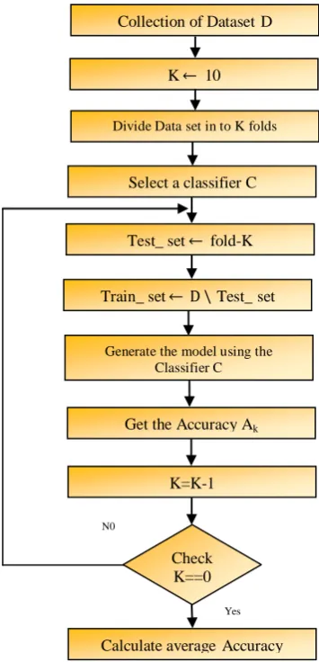
4.2PROPOSED CVMETHOD :

Input D= Training set; K=No folds (assumed K=10 for our experiment); C=Classifier

Select a classifier C

Divide Data set in to K folds

Generate the model using the Classifier C

Calculate averageAccuracy Check

K==0

N0

Yes

Get the Accuracy Ak

Test_ set fold-K

Train_ set D \Test_set

No

Select the classifier C Divide Data set in to 10

folds

Generate the model using the Classifier C

Calculate average Accuracy

Check K==0

Yes

Get the Accuracy Ak

Test_ set fold-K

Train_ set D \ Test_set

K=K-1 K 10(Default value) Collection of Dataset D

Randomize the indices of D

PROPOSED CVMETHOD Divide D in to K folds

Get the mode based on C using K-1 folds

Test the model based on C obtained in the step2 using Kth folds and get the accuracy Ak Generate the random indices for the dataset D

Repeat the testing step 3 using the model step2

OUTPUT

Average accuracy A= ( )/K

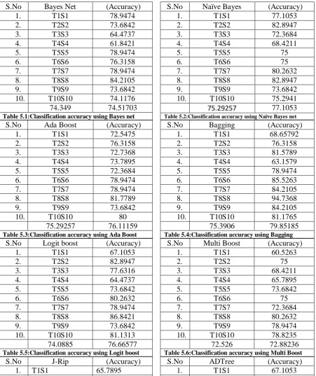
V. EXPERIMENTAL RESULTS

In the following table the partition TiSi represents with Ti, test set 10% and Si, train data 90%. Each Ti or Si is the randomised sub set of original data set.

S.No Bayes Net (Accuracy)

1. T1S1 78.9474

2. T2S2 73.6842

3. T3S3 64.4737

4. T4S4 61.8421

5. T5S5 78.9474

6. T6S6 76.3158

7. T7S7 78.9474

8. T8S8 84.2105

9. T9S9 73.6842

10. T10S10 74.1176

74.349 74.51703

Table 5.1:Classification accuracy using Bayes net

S.No Naïve Bayes (Accuracy)

1. T1S1 77.1053

2. T2S2 82.8947

3. T3S3 72.3684

4. T4S4 68.4211

5. T5S5 75

6. T6S6 75

7. T7S7 80.2632

8. T8S8 82.8947

9. T9S9 73.6842

10. T10S10 75.2941

75.29257 77.1053

Table 5.2:Classification accuracy using Naïve Bayes net

S.No Ada Boost (Accuracy)

1. T1S1 72.5475

2. T2S2 76.3158

3. T3S3 72.7368

4. T4S4 73.7895

5. T5S5 72.3684

6. T6S6 78.9474

7. T7S7 78.9474

8. T8S8 81.7789

9. T9S9 73.6842

10. T10S10 80

75.29257 76.11159

Table 5.3:Classification accuracy using Ada Boost

S.No Bagging (Accuracy)

1. T1S1 68.65792

2. T2S2 76.3158

3. T3S3 81.5789

4. T4S4 63.1579

5. T5S5 78.9474

6. T6S6 85.5263

7. T7S7 84.2105

8. T8S8 94.7368

9. T9S9 84.2105

10. T10S10 81.1765

75.3906 79.85185

Table 5.4:Classification accuracy using Bagging

S.No Logit boost (Accuracy)

1. T1S1 67.1053

2. T2S2 82.8947

3. T3S3 77.6316

4. T4S4 64.4737

5. T5S5 73.6842

6. T6S6 80.2632

7. T7S7 78.9474

8. T8S8 86.8421

9. T9S9 73.6842

10. T10S10 81.1313

74.0885 76.66577

Table 5.5:Classification accuracy using Logit boost

S.No Multi Boost (Accuracy)

1. T1S1 60.5263

2. T2S2 75

3. T3S3 68.4211

4. T4S4 65.7895

5. T5S5 73.6842

6. T6S6 75

7. T7S7 72.3684

8. T8S8 80.2632

9. T9S9 78.9474

10. T10S10 78.8235

72.526 72.88236

Table 5.6:Classification accuracy using Multi Boost

S.No J-Rip (Accuracy)

1. T1S1 65.7895

2. T2S2 78.9474

3. T3S3 69.7368

4. T4S4 61.8421

5. T5S5 75

6. T6S6 80.2632

7. T7S7 76.3158

8. T8S8 85.5263

9. T9S9 71.0526

S.No ADTree (Accuracy)

1. T1S1 67.1053

2. T2S2 78.9474

3. T3S3 71.0526

4. T4S4 59.2105

5. T5S5 77.6316

6. T6S6 76.3158

7. T7S7 78.9474

8. T8S8 81.5789

10. T10S10 75.2941

71.0417 73.97678

Table 5.7:Classification accuracy using J-Rip

10. T10S10 81.1765

72.9167 74.82818

Table 5.8:Classification accuracy using ADTree

S.No Decision Stump (Accuracy)

1. T1S1 70.5263

2. T2S2 72.3684

3. T3S3 70.4211

4. T4S4 70.7895

5. T5S5 71.0526

6. T6S6 77

7. T7S7 67.1053

8. T8S8 72.3684

9. T9S9 69.7368

10. T10S10 77.6471

71.875 71.90155

Table 5.9:Classification accuracy using Decision Stump

S.No J48 (Accuracy)

1. T1S1 68.4211

2. T2S2 80.2632

3. T3S3 71.0526

4. T4S4 59.2105

5. T5S5 77.6316

6. T6S6 85.5263

7. T7S7 81.5789

8. T8S8 97.3684

9. T9S9 78.9474

10. T10S10 78.8235

73.8281 77.88235

Table 5.10:Classification accuracy using J48

S.No Classifiers CV Accuracy Randomize

1. Bagging 75.3906 79.85185

2. Logit boost 74.0885 76.66577

3. Multi Boost 72.526 72.88236

4. J-Rip 71.0417 73.97678

5. ADTree 72.9167 74.82818

6. Decision Stump 71.875 72.00155

7. J48 73.8281 77.88235

8. Bayes Net 74.349 74.51703

9. Naïve bayes 75.29257 77.1053

10. Ada boost 75.29257 76.29159

Table 5.11: Table of summarization of results in tables 5.1 to 5.10

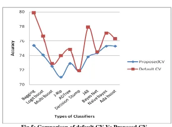
VI.CONCLUSIONS

We find the efficiency of results in randomizing the indices in the process of cross validation. The outputs of our experiments as shown in the Fig 5 proves the achievement of better performance. Specifically even in the small range of data sizes and collection of classifiers we achieve increment 0 to 6%.

Future remarks: The approach proposed in this paper can be further modified with the randomizing the indices as well as varying the learning models in each iteration step. Even though it may lead to cost intensive process, it can be verified in a parallel/distributed computational approach.

ACKNOWLEDGEMENT

The authors would like to thank the management of Annamalai University for the support and encouragement for this research work.

R

[1] V.N. Vapnik. Estimation of dependences based on empirical data. Springer, New York, 1982.

[2] Powers, D.M.W.; Atyabi, A, "The Problem of Cross-Validation: Averaging and Bias, Repetition and Significance," Engineering and Technology (S-CET), 2012 Spring Congress on , vol., no., pp.1,5, 27-30 May 2012

[3] Larson S. The shrinkage of the coefficient of multiple correlation. J. Educat. Psychol., 22:45–55,1931. [4] Mosteller F. and Wallace D.L. Inference in an authorship problem. J. Am. Stat. Assoc., 58:275–309, 1963. [5] Mosteller F. and Turkey J.W. Data analysis, including statistics. In Handbook of Social Psychology.

Addison-Wesley, Reading, MA, 1968.

[6] Stone M. Cross-validatory choice and assessment of statistical predictions. J. Royal Stat. Soc., 36(2):111– 147,1974.

[7] Geisser S. The predictive sample reuse method with applications. J. Am. Stat. Assoc., 70(350):320– 328,1975.

[8] Kohavi R. A study of cross-validation and bootstrap for accuracy estimation and model selection. In Proceedings of International Joint Conference on AI. 1995, pp. 1137–1145, URL http:// citeseer.ist.psu.edu/kohavi95study.html.

[9] Liu H. and Yu L. Toward integrating feature selection algorithms for classification and clustering. IEEE Trans. Knowl. Data Eng., 17(4):491–502,2005, doi:http://dx.doi.org/10.1109/ TKDE.2005.66.

[10] Efron, B. and Morris, C. (1973). Combining possibly related estimation problems (with discussion). J. R. Statist. Soc. B, 35:379.

[11] Efron, B. and Tibshirani, R. (1997). Improvements on cross-validation: the .632+ bootstrap method. J. Amer. Statist. Assoc., 92(438):548–560.

[12] Refaeilzadeh P., Tang L., and Liu H. On comaprison of feature selection algorithms. In AAAI-07 Worshop on Evaluation Methods in Machine Learing II. 2007.

[13] Salzberg S. On comparing classifiers: pitfalls to avoid and a recommended approach. Data Min. Knowl. Disc., 1(3):317–328, 1997, URL http://citeseer.ist.psu.edu/salzberg97comparing.html.

[14] D.Udhayakumarapandian.,RM.Chandrasekaran., andA.Kumaravel “A Novel Subset Selection For Classification Of Diabetes Dataset By Iterative Methods” Int J Pharm Bio Sci ,5 (3) : (B) 1 – 8, July(2014) [15] A.Kumaravel., Udhayakumarapandian.D.,Consruction Of Meta Classifiers For Apple Scab Infections ,

Int J Pharm Bio Sci, 4(4): (B) 1207 – 1213, Oct(2013)

[16] A.Kumaravel., Pradeepa.R., Efficient molecule reduction for drug design by intelligent search methods.Int J Pharm Bio Sci, 4(2): (B) 1023 – 1029,Apr (2013)

[17] https://www.waset.org/journals/waset/v68/v68-21.pdf world academy of science, engineering and technology, 2012.

[18] H.Dunham, Data Mining, Introductory and Advanced Topics, Prentice Hall, 2002 [19] Source about wekahttp://www.cs.waikato.ac.nz/ml/weka/ downloaded on 3rd august 2014 [20] L. Breiman, “ RandomForests,”inMachine Learning, vol. 45, pp. 5-32, 2001.

[21] Steve R. Gunn., University Of Southampton,Support Vector Machines for Classification and Regression. [22] Dietterich, T. G., Jain, A., Lathrop, R., Lozano-Perez, T. (1994). A comparison of dynamic reposing and

[23] A.Stensvand, T. Amundsen, L. Semb, D.M. Gadoury, and R.C. Seem. 1997. Ascospore release and infection of apple leaves by conidia and ascospores of Venturia inaequalis at low temperatures. Phytopathology 87:1046-1053.

[24] Website for attribute description

http://archive.ics.uci.edu/ml/machine-learning databases/pima-indians-diabetes., accessed on 3rd august 2014

[25] Bal,Hp.2005.Bioinformatics-principles and applications.Tata McGraw-Hill Publishing company Ltd New Delhi.

[26] Bo.Th and Jonassen,I-2002 New feature subset selection procedures for classification of expression profiles.Genome Biology 3:research 00170.-0017.11

[27] Khalid AA Abakar & Chongwen Yua., Performance of SVM based on PUK kernel in comparison to SVM based on RBF kernel in prediction of yarn tenacity, Indian Journal of Fibre & Textile Research, Vol. 39: (B) 55-59, March (2014).

[28] Steve R. Gunn., Support Vector Machines for Classification and Regression Technical Report., Faculty of Engineering, Science and Mathematics School of Electronics and Computer Science .,10 May 1998 [29] F. Girosi., An equivalence between sparse approximation and Support Vector Machines.A.I. Memo 1606,

MIT Artificial Intelligence Laboratory, 1997.

[30] N. Heckman., The theory and application of penalized least squares methods or reproducing kernel hilbert spaces made easy, 1997.