Implemented For Distance Measurement Technique Using
Image Processing for Android Application
Mr. Ghumare Amar Ashok , Dr.Jadhavar , Dr.MulajkarR.M
E&TC Department Jaihind college of Engineering, Kuran
B.R., E&TC Department Jaihind college of Engineering, Kuran
E&TC Department Jaihind college of Engineering, Kuran
Abstract
Existing distance measurement methods either require multiple images and special photographing poses or only measure the height with a special view configuration. We propose a novel image-based method that can measure various types of distance from single image captured by a smart mobile device. The embedded accelerometer is used to determine the view orientation of the device. Consequently, pixels can be back-projected to the ground, thanks to the efficient calibration method using two known distances. Then the distance in pixel is transformed to a real distance in centimeter with a linear model parameterized by the magnification ratio. Various types of distance specified in the image can be computed accordingly. Experimental results demonstrate the effectiveness of the proposed method. Index Terms—Accelerometer, distance measurement, single image, smart mobile device.
1. Introduction
Image classification research aims at finding representations of images that can be automatically used to categorize images into a finite set of classes. Typically, algorithms that classify images require some form of pre-processing of an image prior to classification. This process may involve extracting relevant features and segmenting images into sub-components based on some prior knowledge about their context ([1],[2]). Typically in order for the classification to be accurate one needs to choose one of the many methods and algorithms based on whatever side-information that one may have about
the images that one expects to classify. There is no universal best algorithm that is guaranteed to yield high rates of classification for all kinds of problems. However, in the area of text recognition there have recently been new string-distance measures [3],[4] that can compare any two strings of characters without any assumption on their context. These distances have been shown to be successful on a variety of pattern recognition tasks of data clustering and pattern classification. In this paper we introduce a new image distance measure which is based on such string distances. We are able thus to measure distances between any pair of images and do classification and clustering of images without any feature extraction.
mobile device oriented singleimage-based approach for distance measurement, which utilizes the embedded camera and accelerometer for photographing and recovering the scene geometry. 2) A new calibration method based on two known distances is proposed to obtain an accurate focal length, which is simpler and more efficient in comparison with the existing calibration methods. 3) Various types of distances including ground distance, depth, and height can be measured, while the existing methods can only handle one or two types.
2. Literature survey
[1] In this research, a novel vehicle-borne system of measuring three–dimensional (3-D) urban data using single-row laser range scanners is proposed. Two single-row laser range scanners are mounted on the roof of a vehicle, doing horizontal and vertical profiling respectively. As the vehicle moves ahead, a horizontal and a vertical range profile of the surroundings are captured at each odometer trigger. The freedom of vehicle motion is reduced from six to three by assuming that the ground surface is flat and smooth so resulting in the vehicle moving on almost the same.
[2] With the invention of the low-cost Microsoft Kinect sensor, high-resolution depth and visual (RGB) sensing has become available for widespread use. The complementary nature of the depth and visual information provided by the Kinect sensor opens up new opportunities to solve fundamental problems in computer vision. This paper presents a comprehensive review of recent Kinect-based computer vision algorithms and applications. The reviewed approaches are classified according to the type of vision problems that can be addressed or enhanced by means of the Kinect sensor. The covered topics include preprocessing, object tracking and recognition, human activity analysis, hand gesture analysis, and indoor 3-D mapping. For each category of methods, we outline their main algorithmic contributions and summarize their advantages/differences compared to their RGB counterparts. Finally, we give an overview of the challenges in this field and future research trends.
This paper is expected to serve as a tutorial and source of references for Kinect-based computer vision researchers.
[3] Time-of-flight (Tof) imaging based on the photonic mixer device (PMD) or similar ToF imaging solutions has been limited to short distances in the past, due to limited lighting devices and low sensitivity of ToF imaging chips. Long-range distance measurements are typically the domain of laser scanning systems. In this paper, PMD based medium- and long-range lighting devices working together with a 2-D/3-D camera are presented and several measurement results are discussed. The proposed imaging systems suffer from two systematic limitations in addition to problems due to wind and insufficient lighting: a low lateral resolution of the depth imaging chip and ambiguities in the distance measurements. In order to provide a robust and flexible system, we introduce algorithms to obtain unambiguous depth values (phase unwrapping) and to perform a joint motion compensation and super-resolution. Several experiments were conducted in order to evaluate the components of the multimodal imaging system.
3. Proposed method
Fig. 3.1 Pipeline of the proposed method. (a) Scene is captured by a hand-held mobile device to obtain the acceleration data. (b) Camera is calibrated with the view orientation to estimate the magnification ratio. (c) Different types of distance (e.g., depth, height, and ground distance) are measured with the ratio.
3.1 Coordinate Systems
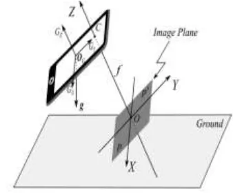
Let us first introduce the coordinate systems used in our method (Fig. 2). OXYZ is the image coordinate system of the device with the focal length f being the distance between the camera optical center C(0, 0, f ) and the origin O(0, 0, 0). For the gravitational acceleration data obtained by the accelerometer, each acceleration datum is a vector consisting of three orthogonally projected elements.
Correspondingly, we can translate the image coordinate system to the device and then obtain the acceleration coordinate system OGGXGYGZ. GX, GY, and GZ are axes corresponding to the three acceleration dimensions with OG being the origin on the device. g in Fig. 2 denotes the gravitation, which is also the norm of ground. Since the accelerometer records the acceleration of the gravitation, for simplicity, we also denote the acceleration data by g in the following paragraphs.
Fig 3.2. Coordinate systems
3.2 Initialization
gravitation in GX, GY, and GZ axes as Fig. 2 shows. Considering the gravitation is vertical to the ground, we can conclude that the view orientation of the device can be computed directly. For the distance measurement, this direction is required for fulfilling the back-projection which helps mapping the pixel distance to the real distance. Therefore, we record the gravitational acceleration when capturing the scene image.
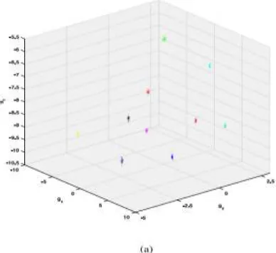
However, the recorded acceleration data are highly unstable with heavy noises due to the unavoidably continuous camera jitter, even when we try our best to hold the device still. Fig. 3(a) shows ten such noisy example acceleration data sets recorded from ten captures. Each capture lasts for one second and is depicted in a different color. In this figure, gx, gy, and gz denote the three elements of each data in GX, GY, and GZ dimensions, respectively. The dots in each set represent the recorded accelerations during the image capture. We can see the noticeable shaky movement of the device during capturing. Apparently, such noisy data cannot be directly used for view direction computation.
The technology has a wide variety of applications, from augmented reality in computer games and apps, to robot interaction, and self-driving cars. Historical images and videos can also be analysed by the software, which is useful for reconstruction of incidents or to automatically convert 2D films into immersive 3D.“Inferring object-range from a simple
image by using real-time software has a whole host of potential uses,” explained supervising researcher, Dr Gabriel Brostow (UCL Computer Science).
Fig 3.3. Examples of gravitational acceleration data denoising. (a) Ten acceleration data sets shown in different colors for ten captures at different positions, with each set being obtained during the one-second photographing duration. (b) Denoised results of the ten data sets shown in (a). Note that the results (shown in dots) in (b) are zoomed in for clear viewing.
We propose a weighted average method to denoise the noisy sensor data. In this method, for a recorded acceleration data set g(t), t ∈ [τ − (T/2), τ + (T/2)] at the exposure time τ, the denoised data g¯ can be computed by weighted averaging all the data during the sample time T
𝑔̅ = 1
∑𝜏+ 𝑤(𝑡)
𝜏 2 𝜏−𝜏 2
∑ 𝑤(𝑡)𝑔(𝑡) (1)
𝜏+2𝜏
𝜏−2𝜏
single datum. The view orientation of the device can then be easily computed with such a datum, which is the basis of back projection for computing the magnification ratio.
3.3 Camera Calibration and Magnification Ratio Estimation
Magnification ratio transforms the distance in pixel to the real distance in centimeter. To compute the magnification ratio e, the pixels specified by the user in the image have to be back projected to the ground. Focal length f is required to perform the back-projection operation, hence, we calibrate the camera first to obtain the focal length. Once we know f , e can be computed with a known distance.
1) Calibrating the Camera: The calibration method uses two unparallel known distances on the ground to estimate f . Normally, we only need to calibrate f once due to the fixed camera lens of most smart devices. Therefore, it is easier to apply compared with the traditional calibration method [29] which requires a checkerboard with multiple images captured.
Assume that the image plane being z = 0 (Fig. 2). The ground can be described as
[𝑔𝑥𝑔𝑦𝑔𝑧𝑑] [
𝑋 𝑌 𝑍 1
] = 0 (2)
where d is a parameter of ground equation and does not affect the measurement results, as explained in Section II-C2. p(px, py, 0) is a pixel corresponding to a ground point P(PX, PY, PZ).
The straight line Cp which passes C and p can be parameterized by t as
{
𝑥′= 𝑡𝑝𝑥
𝑦′= 𝑡𝑝𝑦
𝑧′= −𝑡𝑓 + 𝑓
(3)
P also lies on the straight line Cp and, therefore
𝑃 = [ 𝑃𝑋
𝑃𝑌
𝑃𝑍
] = [
𝑡𝑝 0 0 0
0 𝑡𝑝 0 0
0 0 0 (1 − 𝑡𝑝)𝑓
] [ 𝑝𝑥
𝑝𝑦
0 1 ]
= 𝐻𝑃 (4)
where t p = [(−d − gzf )/(gxpx + gypy − gzf ]. Equation (4) shows that p and P are connected by a transform matrix H. It can be used to compute the pixel distance between two pixels in the image. For instance, for the two pixels p(px, py, 0) and p(px, py, 0) whose back-projection points are P(PX, PY, PZ) and P(PX, PY, PZ), their pixel distance is
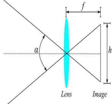
Fig 3.4. Illustration of the principle of the CCD camera. α represents the horizontal or vertical view angle with h being the corresponding width or height of the image.
‖𝑃𝑃1‖ = √(𝑃
𝑋− 𝑃𝑋′) 2
+ (𝑃𝑌− 𝑃𝑌′) 2
+ (𝑃𝑧− 𝑃𝑧′) 2
= 𝑠𝐹(𝑝, 𝑝1, 𝑓). (5)
n (5), s = d + fgzis a scalar and irrelevant to ground point and F(p, p, f ) is a function of p, p, and f
𝐹(𝑝, 𝑝′, 𝑓)
=
√𝐴𝑝𝑝′𝑓2+ 𝐵𝑝𝑝′𝑓 + 𝐶𝑝𝑝′
‖𝐷𝑝𝑝′𝑓2+ 𝐸𝑝𝑝′𝑓 + 𝐹𝑝𝑝′‖
Where
Equation (5) contains two unknown variables, s and f . Therefore, two different distances are required to estimate them. A more convenient way is to compute the ratio between two distances so that s which contains d is eliminated. The left variable f can be computed by PP and another distance QQfor two pixels q and q
‖𝑃𝑃′‖ ‖𝑄𝑄′‖=
𝐹(𝑝, 𝑝′, 𝑓)
𝐹(𝑞, 𝑞′, 𝑓) (7)
Equation (7) is a quartic function that every polynomial equation can be solved by radicals. We propose a robust prediction-based method to estimate f from four roots of (7). It is based on the geometric relationships among focal length, field of view and the image plane of a CCD camera, which is shown in Fig. 4.
The relationship can be formulated as
𝑡𝑎𝑛𝛼
2=
ℎ
2𝑓 (8)
The field of view α is almost fixed while the focal length f changes for this imaging model and, in practice, the horizontal field of view α of the embedded camera is approximately 60. Therefore, a prediction of f , f¯, can be first estimated by setting α = 60◦
𝑓̅ = ℎ
2𝑡𝑎𝑛 (1
2𝛼)
(9)
Then, the one closest to f¯ among the four roots is selected as the finally estimated focal length.
2) Computing the Magnification Ratio: Assume that the relationship between the real distance of two pixels and their corresponding pixel distance is linear. For two pixels p and p, their real distance, Lpp, can be estimated from their pixel distance, PP, via a linear model with a parameter, e called magnification ratio
However, there is no information on the relationship between the real distance and the pixel distance and, therefore, a known distance in centimeter whose pixel distance can be estimated by (5) is required to determine e. Consequently e can be obtained directly by solving (10) as
𝑒 = 𝐿̂𝑝𝑝′
‖𝑝𝑝′‖ (11)
where L pp represents the known real distance with PP being its pixel distance.
Such a known distance can be the ground distance, height or depth so that its pixel distance can be estimated by (5). This condition can be easily satisfied in the real measurement scenario. Furthermore, other kinds of known distance can also be adopted by (11) if some interactions can be taken to estimate its pixel distance (see Section IV for more details).
Although e is scaled by 1/s with the unknown s, the scale does not affect the distance computation. That is, if there is another pair of points u and u, their real distance Luu can be computed by (5), (10), and (11) as follows:
𝐿𝑢𝑢′= 𝑒 ∗ ‖𝑈𝑈′‖ =
𝐹(𝑢, 𝑢′, 𝑓)
𝐹(𝑝, 𝑝′, 𝑓)𝐿𝑝𝑝′ (12)
Apparently, s has no effect on distance measurement, and d included in s is useless as we have claimed before.
3.4 Distance Measurement
Fig. 5 illustrates the three types of distance (ground distance, depth, and height) to measure and their corresponding notations. These three types of distance can be the base distances so that an arbitrary distance can be measured.
Fig 4.5.Illustration of the measurements for different types of distance. Lp1p2 denotes the ground distance between P1 and P2. Hc and Hp1p3 represent the heights of camera and object P1P3 . eCP1, eCP2, and eCP 3are depths of p1, p2, and p3, respectively
1. Ground Distance: Ground distance can be
estimated in a relatively simple way according to the proposed method. For the two example ground points P1 and P2 shown in Fig. 5, their corresponding image pixels are p1 and p2. To compute the ground distance Lp1p2, p1 and p2 are first back projected from the image plane to their ground points P1 and P2 according to (4). Then Lp1p2 can be computed by
𝐿𝑃1𝑃2 = 𝑒 ∗ ‖𝑝1𝑝2‖ =
𝐹(𝑝1𝑝2, 𝑓)
𝐹(𝑝, 𝑝′, 𝑓)𝐿𝑝𝑝′ (13)
2. Depth: Depth is the distance between the camera
optical center and the user-specified point in 3-D space. If the specified point is above the ground, its projection on the ground also has to be specified to determine its position in 3-D space. The depth is also computed with the magnification ratio using (10). For the ground point P1 in Fig. 5 whose corresponding image pixel is p1, its depth of Dp1 can be computed as follows:
It is difficult to compute the depth directly if the specified point is above the ground. For example, for the pixel p3 as shown in Fig. 5, its corresponding point in 3-D space is P 3 with back-projected point P3 on the ground. CP 3, the pixel distance of depth of point p3, cannot be computed directly. However, the
distance between C and P3 can be computed in the similar way as Dp1, supposing that the specified point is on the ground. The length of the line segment P3P 3 also can be obtained with the ground distance Lp1p3 and θ. Then the depth of p3 can be computed according to the geometrical relationship as follows:
𝐷𝑃3 = 𝑒‖𝐶𝑃3
′‖ = 𝑒‖𝐶𝑃
3‖ =
𝐿𝑃1𝑃3
cos (𝜃) (14)
where θ is computed by the principle of the triangle geometry
𝜃 =𝜋
2− 𝑎𝑟𝑐𝑐𝑜𝑠
𝐶𝑃3
⃗⃗⃗⃗⃗⃗⃗ ∗ 𝑔 ‖𝐶𝑃⃗⃗⃗⃗⃗⃗⃗ ‖ ∗ ‖𝑔‖3
3. Height: Two kinds of height can be measured: 1)
camera height and 2) object height. The former means the distance from camera optical center C to the ground while the latter means the distance between two specified points: one for the top of object and the other as the ground position for the bottom.
Similar to the ground distance and depth, the height in pixel has to be computed first and then multiplied by the magnification ratio. For the camera height Hc shown in Fig. 5, whose bottom C is the projection of C on the ground, it can be computed as
𝐻𝑐 = 𝑒 ∗ ‖𝐶𝐶′‖ =
𝐿𝑝𝑝′
𝐹(𝑝, 𝑝′, 𝑓)‖𝑔‖ (15)
For the example object height Hp1p3 as shown in Fig. 5, p1 and p3 are its bottom and top, respectively, with their corresponding back-projected points on the ground being P1 and P3. The corresponding point in 3-D space for p3 is P 3. Consequently, the object height Hp1p3 can be computed as
𝐻𝑃1𝑃3 = 𝑒‖𝑃1𝑃3
′‖ = 𝑒‖𝑃
1𝑃3‖tan (𝜃)
where θ is the angle between the straight line CP3 and the ground
𝜃 =𝜋
2− 𝑎𝑟𝑐𝑐𝑜𝑠
𝐶𝑃3
4. RESULTS
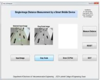
Fig 4.1 Overall Structure of Proposed Work GUI
Fig 4.2 Selected Input Image
Fig 4.3 Gray Scale of Selected Input Image
Fig 4.4 Error 3D plot for the selected input gray scale image
Fig 4.5 Go for Spatial Calibration First
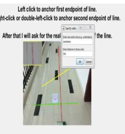
Fig 4.7.First calibrate the input Image(using scale of centimeters)
Fig 4.8. Different operations for Distance Measurement
Fig4.9 Calculated Distance and Its Intensity Profile
5. CONCLUSION
In this paper, we have proposed a novel method for conveniently measuring various distances from a single image captured by a smart mobile device. The accelerometer integrated in the smart device is used to estimate the view direction which thus helps back-projecting the image pixel to the ground. The back projection is performed based on a new camera calibration method which can estimate the focal length accurately with two known distances. Then, the magnification ratio can be computed for converting the pixel distance into real distance. With back-projection and the magnification ratio, various types of distance including ground distance, depth, and height can be measured accurately. Experimental results show the effectiveness of the proposed method. Currently, our method requires a known distance for the measurement. How to measure the distance without the known distance will be considered in our future work.
References
[1] H. Zhao and R. Shibasaki, “A vehicle-borne urban 3-D acquisition system using single-row laser range scanners,” IEEE Trans. Syst., Man, Cybern. B, Cybern., vol. 33, no. 4, pp. 658–666, Aug. 2003.
sensor: A review,” IEEE Trans. Cybern., vol. 43, no. 5, pp. 1318–1334, Jun. 2013.
[3] B. Langmann, W. Weihs, K. Hartmann, and O. Loffeld, “Development and investigation of a long-range time-of-flight and color imaging system,” IEEE Trans. Cybern., vol. 44, no. 8, pp. 1372–1382, Aug. 2014.
[4] Z. Jiang, N. Jiang, Y. Wang, and B. Zang, “Distance measurement in panorama,” in Proc. IEEE Int. Conf. Image Process. (ICIP), San Antonio, TX, USA, 2007, pp. VI-393–VI-396.
[5] M.-C. Lu, W.-Y.Wang, and C.-Y. Chu, “Image-based distance and area measuring systems,” IEEE Sensors J., vol. 6, no. 2, pp. 495–503, Apr. 2006.
[6] C.-M. Wang and W.-Y.Chen, “The human-height measurement scheme by using image processing techniques,” in Proc. Int. Conf. Inf. Security Intell. Control (ISIC), 2012, pp. 186–189.
[7] C.-T. Chuang, W.-Y.Wang, C.-P.Tsai, Y.-H.Chien, and M.-C. Lu, “An image-based area measurement system,” in Proc. Int. Conf. Syst. Sci. Eng. (ICSSE), 2011, pp. 644–648.
[8] M.-C. Lu, C.-C.Hsu, and Y. Y. Lu, “Improvements and application of the image-based distance measuring system,” in Proc. WSEAS Int. Conf. (CISST), 2007, pp. 17–19.
[9] W.-Y. Wang, M.-C.Lu, C.-T.Chuang, and J.-C. Cheng, “Image-based height measuring system,” in Proc. 7th WSEAS Int. Conf. Signal Process.Comput. Geometry Artifical Vis. (ISCGAV), 2007, pp. 147– 152.
[10] T.-H. Wang, M.-C.Lu, W.-Y.Wang, and C.-Y. Tsai, “Distance measurement using single non-metric CCD camera,” in Proc. 7th WSEAS Int. Conf. Signal Process.Comput.Geometry Artif. Vis., 2007, pp. 24– 26.
[11] C.-C. Chen, M.-C.Lu, C.-T.Chuang, and C.-P. Tsai, “Vision-based distance and area measurement system,” WSEAS Trans. Signal Process., vol. 4, no. 2, pp. 36–43, 2008.
[12] N. Pauly and N. I. Rafla, “An automated embedded computer vision system for object measurement,” in Proc. Int. Midwest Symp. Circuits Syst. (MWSCAS), Columbus, OH, USA, 2013, pp. 1108–1111.
[13] M.-C. Lu, C.-C.Hsu, and Y.-Y. Lu, “Image-based system for measuring objects on an oblique plane and its applications in 2-D localization,” IEEE Sensors J., vol. 12, no. 6, pp. 2249–2261, Jun. 2012.