An Efficient Numerical Technique to Calculate the High Frequency
Diffracted Fields from the Convex Scatterers
with the Fock-Type Integrals
Yang Yang1, Yu Mao Wu1, *, Ya-Qiu Jin1, Haijing Zhou2, Yang Liu2, and Jianli Wang3
Abstract—High frequency electromagnetic (EM) scattering analysis from the scatterers is important to the computational electromagnetics community. Meanwhile, high frequency diffraction technique, like the uniform geometrical theory of diffraction (UTD), is very important when the observation point lies in the transition, shadow and deep shadow regions of the considered scatterer. Furthermore, the diffracted fields arising from the scatterers via the UTD technique are usually highly oscillatory in nature, which is named as the Fock type integrals with the Airy function and its derivative involved. In this work, we propose a Fourier quadrature method to calculate the Pekeris integrals. Moreover, we first adopt the Fourier quadrature technique to calculate the diffracted fields from the dielectric convex cylinder with impedance boundary conditions, like the creeping wave fields and NU-diffracted wave fields. On invoking the Fourier quadrature method, the results of total scattered fields at the fixed observation points could achieve 1 dB relative errors. Moreover, numerical results demonstrate that the computational efforts for the oscillatory Pekeris-integrals are independent of wave frequency with the fixed sampling density and integration limit.
1. INTRODUCTION
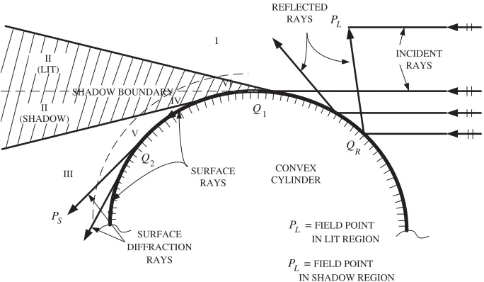
In the computational electromagnetic (CEM) community, efficient methods on calculating the high frequency scattered fields from the scatterers are very important. For instance, high frequency approximation methods including geometrical optics (GO) and physical optics (PO) methods have been widely used to calculate the EM scattered field. The classical GO method only takes effect in the lit region of the considered scatterers. Hence, the diffraction technique is in great need. A geometrical theory of diffraction (GTD) was developed in [1, 2], which accounts for the EM scattered field entering into the shadow region where the GO method fails. Several canonical GTD problems about the edge diffraction, corner or tip diffraction and surface diffracted rays were introduced in [1, 2]. Like the GO method, Keller gave a similar description about diffracted rays and interpreted the phenomenon of diffraction given in detail. Therefore, it could account for the field where geometrical rays cannot exist to overcome the failure of GO field in the shadow region and improve the accuracy in the lit region [3, 4]. Moreover, outside the shadow boundary transition region, the fields via the UTD method automatically are reduced to the fields via the GTD method, which are discussed in [12, 14, 16] for a smooth convex surface with the perfectly conducting boundary condition. The scattering space could be divided into six parts, as shown in Figure 1. It is demonstrated that there are incident and reflected fields in the illuminated region, namely, region I and the lit part of region II. Rays from the lit region traveling along the smooth surface contribute to the diffracted field in the deep shadow part as indicated in the
Received 22 April 2018, Accepted 13 June 2018, Scheduled 31 August 2018 * Corresponding author: Yu Mao Wu ([email protected]).
INCIDENT RAYS
PL
REFLECTED RAYS
SURFACE RAYS
SURFACE RAYS DIFFRACTION
CONVEX CYLINDER I
II
VI IV
III
V (LIT)
II (SHADOW)
SHADOW BOUNDARY
Q
1
2
R Q
Q
PS
P = L FIELD POINT IN LIT REGION
P = L FIELD POINT IN SHADOW REGION
Figure 1. Rays associated with the plane wave scattered by a smooth convex cylinder.
region III and the shadow part of transition region II, which are known as the Watson’s type creeping wave. The subregions IV, V and VI are extremely close to the surface of the convex scatterer. They are commonly referred to as the surface or caustic boundary layer regions. The Taylor series approximation for the canonical Fock integral is available to describe the field in the close regions of the surface. Also, a detailed discussion into the behavior and accuracy of UTD especially in the shadow region of a smooth convex surface is given for a PEC scatterer in [6, 7]. The incremental length diffraction technique, introduced by Shore and Yaghjian [8–10], also provides an efficient way to calculate the high frequency diffracted wave fields.
It is noted that there are several canonical UTD solutions in [11, 13, 15] focusing on smooth convex surfaces with an impedance boundary condition (IBC) which is more practical for predicting the EM scattered fields. The research on the UTD method for electromagnetic fields scattered by a circular cylinder with thin lossy coatings as well as the IBC is of great interest for the EM community. Transition integrals in Pekeris-function form were originally defined by Fock [17]. This kind of integral is formally the Fourier transform of a slowly varying factor comprising a quotient of terms containing Fock-type Airy functions and their derivatives. They are also known as the Fock-type integrals that indicate the mathematical representations of the integrals with the same general features as the Fock functions. Computational application can use the data in tabular form for the case of the PEC. In the general case, a heuristic mean for evaluating the Pekeris integral functions has been explored to represent the Green’s function from a coated cylinder [11]. A uniform GTD treatment procedure of surface diffraction of impedance and coated cylinder by using the residue series technique was introduced in [18] which requires the knowledge of the pole locations. Also, the numerical steepest descent path (NSDP) method [19–23] could be applied to compute the high-frequency PO scattered fields with frequency-independent computational effort and error controllable accuracy.
of integrals in the UTD solution along the transition region provides a simple way for the EM scattering of a circular cylinder for the special two dimensional (2-D) situation.
The main contribution of this work is that the efficient Fourier quadrature technique is adopted to calculate the high frequency scattered fields from both the perfectly conducting and dielectric convex scatterers. This paper is organized as follows. Section 2 gives a vivid depiction about the traveling of rays and introduces the UTD solution in a scalar form. The situation for the electromagnetic scattered by a PEC and impedance circular cylinder is illuminated by an incident plane wave [25] which contains both TM and TE Pekeris functions. In Section 3, the quadrature scheme for these Pekeris functions and the numerical results of the integrals are presented. Then, the UTD solution in Section 2 is computed by using the quadrature scheme and compared with the exact eigenfunction solution in Section 4. The final section summaries the UTD method and numerical procedure in this work. A time dependence of
ejωt is assumed and suppressed throughout the analysis.
2. THE DIFFRACTION PROBLEM FROM THE CONVEX SCATTERER
In this section, a canonical diffraction problem for the EM scattered from a circular cylinder with normal incident plane wave is considered. As known in [26], the plane wave in a homogeneous medium could be decomposed into its TE and TM components, respectively. To make the solution simpler, we consider TMz and TEz incident plane waves where z is the axis of the cylinder. Suppose that an infinitely long circular cylinder is placed at the origin point with the cylinder axis parallel to the z axis of the coordinate system in the free space. The incident TMz/TEz plane waves could be described as
uinc=u0ejkx =u0ejkρcosφ (1)
where the wave amplitude u0 is a complex constant with the cylindrical coordinates (ρ, φ) as shown in
Figure 2. When the EM wave is incident upon the perfectly conducting cylinder, it induces an electric current on the surface of the cylinder, which radiates a secondary scattered field [27]. The superposition of the incident fielduincand scattered field usca gives us the total field, namely, utot =uinc+usca. The diffracted ray theory was developed based on GO to give a reasonable explanation about the contribution of usca in the shadow region [1, 2]; however, it fails in the transition region. To remedy this limitation, uniform asymptotic results that work well are given in both the shadow and lit parts of the transition regions of the convex scatterer [5].
x y
O
uinc
Ps
s
s'
a Q
Q2 1
Q' Q'
1 2
θ ϕ
ρ φ
Figure 2. Ray paths in the shadow regions of the convex cylinder.
-3 -2 -1 0
0.2 0.4 0.6 0.8 1
-3 -2 -1 0
10 20 30 40 50
Phase of
F
(
X
) (degrees)
Phase Magnitude
1 0
Argument X
Magnitude of
F
(
X
)
F(X) = 2j Xe jX∫ ∞ e dτ X
-jτ2
Figure 3. Behaviors of the magnitude and phase of transition functionF(X) as a function of X.
2.1. Shadow Part of the Transition Region of the Considered Scatterer
incident plane wave gazes at Q1 and propagates along the surface ray path, which is known as the
geodesic curve. After reaching Q2, the rays detach the cylinder and propagate in the free space. The
scheme of the diffracted ray could be described in a simple way with the field at attachment pointQ1
multiplying the diffraction coefficients, the spatial attenuation and the phase factor as follows [5]
u(Ps)∼ −u(Q1)p
2
k ·e
−jkt
e−j(π/4)
2ξ√π [1−F(kLa)] +Ps,h(ξ)
e−jks (2)
where uinc(Q1) =u0, t=aθ, ξ =pθ ≥0,p = (ka/2)1/3 and s2 =ρ2−a2. The wave number k in free
space is ω√μ0ε0, and the function F(X) is known as the Fresnel transition function, as discussed for
the edge diffraction analysis [28]. The asymptotic expressions are adopted to compute the transition function F(X) for small (X < 0.3) and large (X > 5.5) parameters X, while a linear interpolation scheme is used for the intermediate values (0.3 ≤ X ≤ 5.5) [28]. Figure 3 gives us the behaviors of magnitude and phase of the transition function F(X) as a function ofX.
The parameters of the Fresnel transition function in Eq. (2) are defined as follows:
L=s, a=θ2/2 (3)
The Pekeris function Ps,h(ξ) is the Fock-type integral defined by
Ps,h(ξ) = e
−j(π/4)
√
π
∞
−∞
QV(τ)
Qw2(τ)
e−jξτdτ =
p∗(ξ)
q∗(ξ) − 1 2√πξ
e−j(π/4) (4)
with
Q=
1, for the TM case,
∂
∂τ, for the TE case. (5)
It is noted that the Pekeris functions in Eq. (4) are obtained under a circular conducting cylinder both for the TMz (soft case) and TEz (hard case) normal incident plane waves with the subscriptss andh. The above equation gives us uniform results around the shadow boundaries of the transition region.
2.2. Lit Part of the Transition Region
For the observation points lying in the lit region, the superposition of the incident fielduincand scattered (reflected) field uref give the total field, namely, utot = uinc+uref, as shown in Figure 4. We could use the usual geometrical optics (GO) field uGO to describe the scattered field in the deep lit region by multiplying the field at QR with the reflection coefficient, spatial attenuation, and phase factor. The
Fresnel reflection coefficients of plane waves reflected from perfected conducting plane surfaces are ±1 which could be obtained by Snell’s law. However, it is noted that the GO representation fails at caustics
as well as in the shadow region. The uniform solution which is valid within the lit region (including the lit part of the transition region) was introduced as follows [5]:
u(PL)uinc(PL)+uinc(QR)
−
−4
ξ ·e
−j(ξ12)3
e−j(π/4)
2ξ√π
1−FkLa+Ps,h(ξ) ρ γ
ργ+le
−jkl (6)
Here, the functions F(X) andPs,h(ξ) are the Fresnel transition function and Pekeris function defined in Equations (2) and (4), respectively. It is noted that the parameters in Equation (6) are different from those in the shadow region distinguished with a superscript, and expressed as
ξ =−2pcosθi ≤0 (7)
whereθi is the incident angle as well as the reflected angle as shown in Figure 4, and
L =l, a = (ξ
)2
2p2 = 2cos 2
θi, ργ = acosθ
i
2 (8)
It is observed that l is the distance of the reflected ray path from QR to PL, and ργ is the reflected ray caustic distance. For the observation pointr far away from the shadow boundary in the lit region,
F(kLa)→1 whileξ 0. In this situation,Ps,h(ξ) could be expressed in an asymptotic approximation
form as
Ps,h(ξ) ±
−ξ
4 e
j(ξ12)3, ξ 0 (9)
Thus, the field in the deep lit region is reduced to
u(PL)u(PL)∓uinc(QR)
ργ
ργ+le
−jkl=u(P
L) +uinc(QR)Rs,h
ργ
ργ+le
−jkl (10)
whereRs,h=∓1 is the surface reflection coefficient corresponding to the TMz/TEzcases. Moreover, the
uniform result will be reduced to the GO solution in the deep lit region. The second term contribution is simple by multiplying the field at QR with the reflection coefficients, spatial attenuation and phase
factor to represent the field propagating along the reflected ray path fromQR to PL.
2.3. The UTD Solution for the IBC Circular Cylinder
Meanwhile, the computation of EM scattering with the impedance boundary condition (IBC) is very important. It is convenient to express the boundary condition of a UTD solution for the EM scattered by a circular impedance cylinder illuminated by the normal incident plane wave as [29, 30]
∂Ez
∂r −jkCT MEz = 0 (11)
for the TMz field and
∂Hz
∂r −jkCT EHz= 0 (12)
for the TEz field, whereCT E =Zs/η0,CT M =Zs/η0, andZsis the surface impedance constant. Under
the new impedance boundary conditions, the total field could also be expressed as the UTD form [11]. Following the same procedure as given in Eqs. (2) and (6), Ps,h(ξ) and Ps,h(ξ) could be replaced by
P(X, q) = e
−j(π/4)
√
π
∞
−∞
V(t)−qV(t)
W2(t)−qW2(t)e
−jXtdt (13)
where q depends on the impedance of the surface and the local radius of the curvature, with the expression as q= ⎧ ⎪ ⎪ ⎪ ⎨ ⎪ ⎪ ⎪ ⎩ −j ka 2
1/2
Zs
η0,
for the TE case,
−j
ka
2
1/2
η0
Zs, for the TM case.
where Zs is the surface impedance and η0 =
μ0/ε0, namely as the characteristic impedance in the
free space. The index q is divided into TM and TE cases, respectively. The parameterX is associated with the angular coordinate of the observation point corresponding toξ in Eq. (2) or ξ in Eq. (6). The pointX = 0 defines the point along the shadow boundary. And the observation points withX <0 and
X >0 lie in the lit region and shadow region in Figure 1, respectively.
3. THE EFFICIENT NUMERICAL METHOD FOR CALCULATING THE FOCK-TYPE INTEGRAL
The uniform results in Eqs. (2) and (6) for the circular cylinder could be readily computed except for the Fock type integrals. The computation of the Fock-type is one of the main contributions in this paper. These kinds of integrals were originally derived by Fock [17], which are associated with the field diffracted by a locally cylindrical impedance surface. In this paper,W1,2(t) andW1,2(t) in Eq. (13) are
the Fock-type Airy functions and their derivatives with respect to the argument t. V(t) and V(t) are defined by
2jV(t) =W1(τ)−W2(t). (15)
It is noted that the Pekeris function in Eq. (13) with respect to the IBC cylinder is the general case. Specifically, we consider the Pekeris function in Eq. (13). The integral P(X, q) is singular as X → 0. One may extract the singular part by splitting the integration path in Eq. (13) into separate parts over (−∞,0) and (0,∞). After substituting Equation (15) into Equation (13), we can get
V(t)−qV(t)
W2(t)−qW2(t)
= 1 2j
W1(t)−qW1(t)
W2(t)−qW2(t) −
1
(16)
Hence,
P(X, q) =e
−j(π/4)
√
π
− 1
2X+
1 2j·
0
∞e−j2π/3
W1(t)−qW1(t)
W2(t)−qW2(t)e
−jXtdt+ ∞
0
V(t)−qV(t)
W2(t)−qW2(t)e
−jXtdt (17)
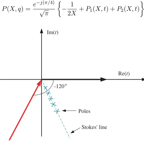
It is indicated from the definition that the integrand of (17) decays as|t| → ∞with arg(t)∈(−π,−2π/3) so that the lower limit of the integration could be changed from−∞to∞e−j2π/3. Hence, the integration path for the function in Eq. (17) is deformed along the path where the Airy function decays fastest, as shown in Figure 5. The asymptotic behavior of the integrand appearing in Eq. (17) is easily viewed by expressing the Fock-type Airy functions as the Miller-type Airy functions
P(X, q) = e
−j(π/4)
√
π
− 1
2X +P1(X, t) +P2(X, t)
(18)
Im(t)
Re(t)
-120o
Poles
Stokes' line
with
P1(X, q) = e
−j(π/6)
2 ·
∞
0
e−j(π/6)Ai(t) +qej(π/6)Ai(t)e−jXrt
ej(π/6)Ai(tej(2π/3)) +qe−j(π/6)Ai(tej(2π/3))dt (19)
and
P2(X, q) =−
1 2·
∞
0
(Ai(t)−qAi(t))e−jXt
ej(π/6)Ai(te−j(2π/3)) +qe−j(π/6)Aite−j(2π/3)dt (20)
The asymptotic approximation forms of the Airy functionAi(t) and its derivativeAi(t) can be arrived at
Ai(t) ∼ 1
2π1/2z1/4e
(−2z3/2)/3
, (21)
and
Ai(t)∼ − z
1/4
2π1/2e
(−2z3/2)/3
, for|arg(t)|< π (22)
In the integral P1, after substituting the integration variable t with te−j2π/3 and applying
r = e−j2π/3 in the exponential function, we can transform the complex path integral with the path parameter t∈ [0,∞). However, this transformation makes the exponential have a parameter r and is not a Fourier transform form. The properties of the transcend integrals depend on the Airy functions and their derivatives involved in the denominator of the integrands. We could take the integration path through the saddle point and leave it along the line of the increasing of the magnitude of the the exponential part e(−2z3/2)/3 in Eqs. (21) and (22). The magnitude of the exponential part e(−2z3/2)/3
of Eqs. (21) and (22) increases while the phase of the exponential part remains constant as |t| → ∞
along the rays with arg(t) = ±2π/3. Hence, the Miller-type Airy function and its derivative decay fast according to the asymptotic approximation form. The Airy functions are not oscillatory along these extreme paths while the e−jXrt factor is seen to produce oscillations with respect to t, whose rate depends on X. Fortunately, this kind of oscillations produced by the imaginary part of r will be overridden by the decay factor involved in the Airy function. Hence, we can use a method like the steepest descent path method according to the work in [24].
Now, we present a quadrature scheme for the integral formed as the following form
I(x) =
NT
0
f(t)e−jXrtdt (23)
Equation (20) fits this form if r is replaced by unity in Eq. (23). The properties of the integrands in Eqs. (19) and (20) ensure the existence of the associated integrals. The slowly varying functionf(t) is further approximated by a piecewise linear function
f(t)f(0)Λ0(t) + N
n=1
f(tn)Λn(t) (24)
where
Λn(t) =
⎧ ⎪ ⎪ ⎪ ⎨ ⎪ ⎪ ⎪ ⎩
t−tn−1
T , t∈(tn−1, tn) tn+1−t
T , t∈(tn, tn+1)
0, otherwise
(25)
and
Λ0(t) =
t
1−t
T , t∈(0, t1)
0, otherwise
(26)
integration here. After substituting Eq. (25) into Eq. (23), we express the integral in a approximation form
I(X)f(0)IΛ0(X) +IΛ0(X) N
n=1
f(tn)e−jnXT r (27)
where
IΛ0(X) =
T
0
Λ0(t)e−jXtrdt= 1
jXr −
e−jXT r
T(Xr)2 + 1
T(Xr)2 ∼
T
2, asX →0 (28)
and
IΛ0(X) =
T
−T Λ0(t)e
−jXtrdt=Tsin2(XT r/2)
(XT r/2)2 (29)
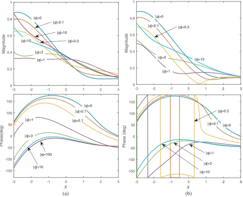
We present the approximation results for the Pekeris function in Eq. (13) as parameter q varies. Specifically, we vary the parameter q along the two paths arg(q) = −π/4 and arg(q) = −3π/4, respectively. Figures 6(a)–6(b) display the Pekeris transition functions as |q| varies from 0 to 10 for arg(q) = −π/4 and arg(q) = −3π/4, respectively. For convenience, we get rid of the singular term
-3 -2 -1 0 1 2 3
0 0.2 0.4 0.6 0.8 1
Magnitude
-3 -2 -1 0 1 2 3
X
-150 -100 -50 0 50 100 150
Phase(deg)
|q|=1 |q|=3
|q|=0.1
|q|=0.3 |q|=10
|q|=10 |q|=0
|q|=0
|q|=0.1
|q|=0.1 |q|=1
|q|=3
|q|=10 |q|=100
-3 -2 -1 0
0 0.2 0.4 0.6 0.8 1
Magnitude
-3 -2 -1 0
X
-150 -100 -50 0 50 100 150
Phase (deg)
|q|=1 |q|=3
|q|=10 |q|=0.3
|q|=0.3 |q|=0
|q|=0 |q|=0.1
|q|=0.1
|q|=1
|q|=3
|q|=10
1 2 3
1 2 3
(a) (b)
Figure 6. The function e−jπ/4(P1+P2)/ √
-3 -2 -1 0 1 2 -0.8
-0.6 -0.4 -0.2 0 0.2 0.4 0.6
Real component
Imaginary component
-3 -2 -1
-1 -0.5 0 0.5 1
Imaginary component
Real component
(a) (b)
ξ ξ
e p
(
ξ
)
-jπ
/4
*
e q
(
ξ
)
-jπ
/4
*
P (ξ) = [p (ξ) - ]1 e-j(π/4) 2 π ξ *
s
P (ξ) = [q (ξ) - ]1 e-j(π/4) 2 π ξ *
h
0 1 2
Figure 7. The real and imaginary parts of the function (a)e−jπ/4p∗(ξ) and (b)e−jπ/4q∗(ξ) in Eq. (4).
1/(2X) directly. Figures 7(a)–7(b) demonstrate Pekeris functions Ps,h(ξ) of PEC cylinder in terms of
related functions.
This algorithm is convenient for engineering applications with two parameters for the evaluation of a given integral: the sampling intervalT and the upper limitN T. The influence of truncation could be obtained by an analytical terms relative to the decay rate of the integrand. The influence of the sampling interval could be obtained by numerical experiments which is relative to the variation rate of the slowly varying function f(t). In this work, to reach an acceptable accuracy, a reasonable choice of sampling density and upper limitT = 0.1 andN T = 18 are adopted.
4. NUMERICAL RESULTS AND DISCUSSIONS
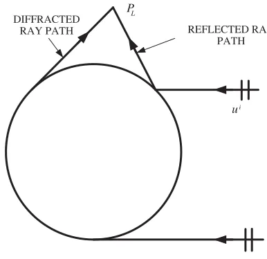
Before evaluating the accuracy of the UTD solution in this paper, the diffracted ray fields in the lit region are taken into consideration to improve the optical ray solutions. Actually, the diffracted rays not only exist in the shadow region, but also have contributions in the lit region, as shown in Figure 8.
PL
REFLECTED RAY PATH DIFFRACTED
RAY PATH
ui
-15 -10
-5 0 10
30
210
60
240
90
270 120
300 150
330
180 0
EIGENFUNCTION SOLUTION UTD
-15 -10
-5 0 5
30
210
60
240
90
270 120
300 150
330
180 0
ENGINFUNCTION SULOTION UTD
(a) (b)
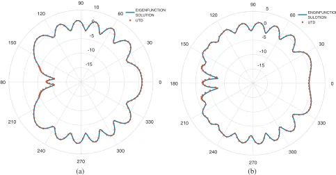
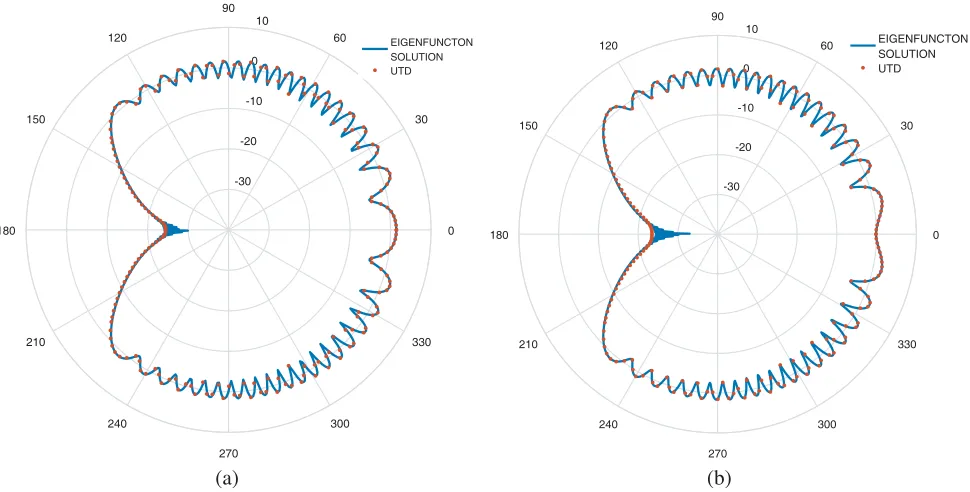
Figure 9. Total scattered field surrounding the circular conducting cylinder of Figure 2 and Figure 4 excited by the (a) TMz and (b) TEzplane wave as a function ofφwithφ = 0, the radius of the cylinder isa= 1.59λ, ρ= 4.76λ.
It is noted that the creeping waves propagate along the surface of cylinder with a spatial attenuation (spreading factor) and decay rapidly. Hence, the total field is actuallyutot =uinc+uref+udiff withudiff
as the higher order diffracted ray field contributions. A few numerical results of circular conducting and impedance cylinder are given in Figures 9(a)–10(b). The reason of the scattered fields obtained by the UTD method agreeing well with the eigenfunction solutions is that the high frequency diffracted fields via the Pekeris integrals are considered in success. Furthermore, the proposed Fourier quadrature technique can compute the Pekeris integral efficiently.
To assess the scattered fields of the UTD solution quantitatively and precisely, we simply fix the observation point in Figure 9(a) with polar angle φ= 2π/3 lying in the transition region. The radius of cylinder is a = 1.59λ. Figure 11 shows the total fields for both the exact eigenfunction solution and the Fourier quadrature technique with wave number kranging from 50 to 150. Relative errors are also given between these two methods. It is observed that the results of total fields using the Fourier quadrature technique can only have 1 dB relative error. Figure 12 demonstrates the consumed time about the aforementioned computation process. It is shown that the Fourier quadrature technique is frequency-independent because of the constant sampling density T and the integral upper limit N T.
-30 -20
-10 0 10
30
210
60
240
90
270 120
300 150
330
180 0
EIGENFUNCTON SOLUTION UTD
-30 -20
-10 0
10
30
210
60
240
90
270 120
300 150
330
180 0
EIGENFUNCTON SOLUTION UTD
(a) (b)
Figure 10. Total scattered field surrounding the impedance circular cylinder of Figure 2 and Figure 4 excited by the (a) TMz and (b) TEz plane wave as a function of φwith φ = 0, the radius of cylinder isa= 15λ,ρ= 25λ, the impedance have the valuesZs/η0 = 1.5j.
50 100 150
-5 0 5
Total Field (dB)
EIGENFUNCTION SOLUTION UTD
50 100 150
k
-1 -0.5 0 0.5 1
Relative Error (dB)
Figure 11. Total scattered field and relative error between eigenfunction and the UTD solution of an impedance circular cylinder excited by the TMz plane wave as a function of wave numberk
with φ= 2π/3, the radius of cylinder is fixed on
a= 1.59λ,ρ= 4.76λ,Zs/η0 = 0.25j.
50 100 150
k 0.02
0.03 0.04 0.05 0.06 0.07 0.08
CPU Time (Second)
EIGENFUNCTION SOLUTION UTD
Figure 12. Comparison of CPU time with eigenfunction solution as a function of wave numberkwith observation point fixed on (φ, ρ) = (2π/3,4.76λ), the radius of cylinder isa= 1.59λ,
5. CONCLUSION
In this work, we have analyzed the high-frequency scattered fields from the convex cylinder. The UTD method for computing the electromagnetic scattered fields of the perfect conducting and dielectric cylinder can significantly improve the solutions of the GO and GTD methods in the shadow region. Then, the Pekeris-integral which usually aries from the high frequency diffracted fields from the body via the UTD technique is considered. We propose the Fourier quadrature technique to calculate these Pekeris integrals which is usually difficult to calculate. Numerical results demonstrate that the Fourier quadrature technique based UTD method can achieve the frequency-independent computation effort and error controllable accuracy. These facts allow us to compute the scattered field from the objects. Finally, the Fourier quadrature technique to calculate the high frequency scattered fields from the convex scatterers is adopted in this work.
ACKNOWLEDGMENT
This work was supported in part by the Science Challenge Program (No. JCKY2016212A502), National Natural Science Foundation of China under Grant No. 11571196, Fudan University, CIOMP Joint Fund, Academy for Engineering and Technology, Fudan University.
REFERENCES
1. Keller, J. B., “Diffraction of a convex cylinder,” IEEE Trans. Antennas Propag., Vol. 4, No. 3, 312–321, 1956.
2. Keller, J. B., “Geometrical theory of diffraction,” J. Opt. Soc. Am., Vol. 52, No. 2, 116–130, 1962. 3. Wu, T. T., “High frequency scattering,” Phys. Rev., Vol. 104, 1201–1212, Dec. 1956.
4. H¨onl, H., A. W. Maue, and K. Westpfahl,Theory of Diffraction, Springer-Verlag, 1961.
5. Pathak, P. H., W. D. Burnside, and R. J. Marhefka, “A uniform gtd analysis of the diffraction of electromagnetic waves by a smooth convex surface,” IEEE Trans. Antennas Propag., Vol. 28, No. 5, 631–642, 1980.
6. Hussar, P. and R. Albus, “On the asymptotic frequency behavior of uniform GTD in the shadow region of a smooth convex surface,” IEEE Trans. Antennas Propag., Vol. 39, No. 12, 1672–1680, 1991.
7. Paknys, R., “On the accuracy of the UTD for the scattering by a cylinder,”IEEE Trans. Antennas Propag., Vol. 42, No. 5, 757–760, 1994.
8. Yaghjian, A. D., R. A. Shore, and M. B. Woodworth, “Shadow boundary incremental length diffraction coefficients for perfectly conducting smooth, convex surfaces,”Radio Sci., Vol. 31, No. 6, 1681–1695, Nov.–Dec. 1996.
9. Hansen, T. B. and R. A. Shore, “Incremental length diffraction coefficients for the shadow boundary of a convex cylinder,” IEEE Trans. Antennas Propag., Vol. 46, No. 10, 1458–1466, Oct. 1998. 10. Shore, R. A. and A. D. Yaghjian, “Shadow boundary incremental length diffraction coefficients
applied to scattering from 3-D bodies,” IEEE Trans. Antennas Propag., Vol. 49, No. 2, 200–210, Feb. 2001.
11. Kim, H. T. and N. Wang, “UTD solution for electromagnetic scattering by a circular cylinder with thin lossy coatings,” IEEE Trans. Antennas Propag., Vol. 37, No. 11, 1463–1472, 1989.
12. Brick, Y., V. Lomakin, and A. Boag, “Fast direct solver for essentially convex scatterers using multilevel non-uniform grids,”IEEE Trans. Antennas Propag., Vol. 62, No. 8, 4314–4324, 2014. 13. Syed, H. H. and J. L. Volakis, “High-frequency scattering by a smooth coated cylinder simulated
with generalized impedance boundary conditions,” Radio Sci., Vol. 26, No. 5, 1305–1314, 1991. 14. Chen, X., S. Y. He, D. F. Yu, H. C. Yin, W. D. Hu, and G. Q. Zhu, “Geodesic computation on
15. Tokgoz, C. and R. J. Marhefka, “A UTD based asymptotic solution for the surface magnetic field on a source excited circular cylinder with an impedance boundary condition,”IEEE Trans. Antennas Propag., Vol. 54, No. 6, 1750–1757, 2006.
16. Ruan, Y. C., X. Y. Zhou, J. Y. Chin, T. J. Cui, Y. B. Tao, and H. Lin, “The UTD analysis to EM scattering by arbitrarily convex objects using ray tracing of creeping waves on numerical meshes,”
Proc. IEEE Antennas Propag. Soc. Int. Symp., 1–4, 2008.
17. Fock, V. A.,Electromagnetic Diffraction and Propagation Problems, Pergamon, New York, 1965. 18. Hussar, P. E., “A uniform GTD treatment of surface diffraction by impedance and coated
cylinders,” IEEE Trans. Antennas Propag., Vol. 46, No. 7, 998–1008, 1998.
19. Wu, Y., L. J. Jiang, and W. C. Chew, “An efficient method for computing highly oscillatory physical optics integral,”Progress In Electromagnetics Research, Vol. 127, 211–257, 2012.
20. Wu, Y. M., L. J. Jiang, and W. C. Chew, “Computing highly oscillatory physical optics integral on the polygonal domain by an efficient numerical steepest descent path method,”J. Comput. Phys., Vol. 236, 408–425, Mar. 2013.
21. Wu, Y. M., L. J. Jiang, W. E. I. Sha, and W. C. Chew, “The numerical steepest descent path method for calculating physical optics integrals on smooth conducting surfaces,” IEEE Trans. Antennas Propag., Vol. 61, No. 8, 4183–4193, Aug. 2013.
22. Wu, Y. M., L. J. Jiang, W. C. Chew, and Y. Q. Jin, “The contour deformation method for calculating the high-frequency scattered field by the Fock current on the surface of the 3-D convex cylinder,”IEEE Trans. Antennas Propag., Vol. 63, No. 5, 2180–2190, 2015.
23. Wu, Y. M., W. C. Chew, Y. Q. Jin, L. J. Jiang, H. Ye, and W. E. I. Sha, “A frequency-independent method for computing the physical optics-based electromagnetic fields scattered from a hyperbolic surface,” IEEE Trans. Antennas Propag., Vol. 64, No. 4, 1546–1552, 2016.
24. Pearson, L. W., “A scheme for automatic computation of fock-type integrals,” IEEE Trans. Antennas Propag., Vol. 35, No. 10, 1111–1118, 1987.
25. Aguilar, A. G., P. H. Pathak, and M. Sierra-Perez, “A canonical UTD solution for electromagnetic scattering by an electrically large impedance circular cylinder illuminated by an obliquely incident plane wave,” IEEE Trans. Antennas Propag., Vol. 61, No. 10, 5144–5154, 2013.
26. Chew, W. C.,Waves and Fields in Inhomogeneous Media, IEEE Press, New York, 1995. 27. Jin, J. M., Theory and Computation of Electromagnetic Fields, Wiley, 2010.
28. Kouyoumjian, R. G. and P. H. Pathak, “A uniform geometrical theory of diffraction for an edge in a perfectly conducting surface,” Proc. IEEE, Vol. 62, No. 11, 1448–1461, 1974.
29. Senior, T. B. A., “Approximate boundary conditions,” IEEE Trans. Antennas Propag., Vol. 29, No. 5, 826–829, 1981.
![Figure 2. When the EM wave is incident upon the perfectly conducting cylinder, it induces an electriccurrent on the surface of the cylinder, which radiates a secondary scattered field [27]](https://thumb-us.123doks.com/thumbv2/123dok_us/1916447.1251416/3.612.312.551.489.630/incident-perfectly-conducting-cylinder-electriccurrent-cylinder-secondary-scattered.webp)