Estimation of the Population Variance Using a Smoothing Operator Under Simple Random Sampling

ESTIMATION OF THE POPULATION VARIANCE USING A SMOOTHING OPERATOR UNDER SIMPLE RANDOM SAMPLING

Lavender Akoth Odhiambo

(BSC Actuarial Science)

I56/PT/CTY/27344/2013

Department of Mathematics and Actuarial Sciences

A Project Submitted in Partial Fulfillment of the Requirements for the Award of the Degree of Master of Science (Statistics) in the School of Pure and Applied Sciences of Kenyatta University

Declaration

This project is my original work and has not been submitted to any other university for examination.

Signature... Date... Lavender Akoth Odhiambo

This project has been submitted for examination with my approval as the university supervisor.

Signature... Date... Dr. Christopher Ouma Onyango

Kenyatta University

This project has been submitted for examination with my approval as the university supervisor.

Signature... Date... Prof.Romanus Odhiambo Otieno

Dedication

Acknowledgment

Table of Contents

Declaration ii

Dedication iii

Acknowledgment iv

List of Tables . . . vii

List of Figures viii List of Appendices ix List of Abbreviations and Acronyms ix Abstract x 1 Introduction 1 1.1 Background of the Study . . . 1

1.2 Problem Statement . . . 2

1.3 Objectives of the Study . . . 3

1.3.1 General Objective . . . 3

1.3.2 Specific Objectives . . . 3

1.4 Significance of Study . . . 3

2 Literature Review 5 2.1 Introduction . . . 5

2.1.1 Review of Estimation Methods . . . 6

2.1.2 Nonparametric regression estimator of the population variance 7 2.1.3 Selection of the Kernel Function . . . 8

2.3 Comparison of the relative efficiency of existing variance estimators . 14

2.4 Research Gap . . . 16

3 Research Methodology 17 3.1 Introduction . . . 17

3.2 Estimation of Variance . . . 17

3.3 The variance of the ratio estimator under robust variance structure of the population mean . . . 17

3.4 Multiplicative bias robust variance estimator for ratio estimator using a smoother function . . . 20

3.5 Asymptotic Unbiasedness of the MBC Estimator . . . 23

3.6 Asymptotic Variance of the MBC estimator . . . 26

3.7 Asymptotic Mean squared of the MBC estimator . . . 27

4 Empirical Study 28 4.1 Introduction . . . 28

4.2 Simulation Procedure . . . 28

4.3 Simulation Results . . . 29

4.4 Real data analysis of the population . . . 30

4.5 Comparison of simulated data and real data . . . 32

4.6 Conclusion . . . 33

4.7 Recommendation for further study . . . 33

References 34

Appendix I: Multiplicative Bias Correction Simulation 37

Appendix II:Conditional Bias Regression 37

List of Tables

2.1 Efficiency Relative to Epanechnkov Kernel . . . 9 4.1 Unconditional biases and RMSE from simulated data . . . 29 4.2 Summary of the unconditional coverage probabilities from the simulted

data. . . 29 4.3 Unconditional biases and RMSE from actual data . . . 32 4.4 Summary of the unconditional coverage probabilities from the actual

List of Figures

List of Abbreviations and Acronyms

s Sample proportion

r Non sample proportion

p−s Non sample space

i Sample element

j Non sample element

n Sample size

N Population size

x Auxiliary variable

y Study variable

f Sampling fraction

ei Error term

p population size

k(t) Kernel function

Var Variance

iid Independent and identically distributed BLUE Best Linear Unbiased Estimator

SRSWR Simple random sampling without replacement MSE Mean Squared Error

RMSE Root Mean Squared Error MBC Multiplicative Bias Correction

UN United nations

Abstract

Chapter 1

Introduction

This chapter presents the background of the study, problem statement, objectives of the study and the significance of the study.

1.1

Background of the Study

The main aim in estimation theory is using sample data to estimate parameters of the population. Experimenters are always interested in using methods which improves precision of population parameters estimates. These parameters can be variance of the population, proportions and means of some characters of study.

Auxiliary information can be applied at both the estimation and selection stages to improve the design and achieve more efficient estimators. For instance, increased precision can be obtained when study variable Y is highly correlated with the auxiliary variable X.

Ratio estimation considers the correlation between the auxiliary variable X and the study variable Y. Whenever positively correlated information is available on the auxiliary variable and the study variable, the ratio estimator is the most suitable for estimating the population variance. For ratio estimators in sampling theory, pop-ulation information of the auxiliary variable such as the coefficient of variation or the coefficient of kurtosis is often used to increase the efficiency of the estimation for the population variance. It therefore follows that a model based approach can be used to increase precision of the estimators by incorporating auxiliary variables. As an approach to such a problem, a superpopulation model is used to describe the relationship between the auxiliary and study variable.

method is applicable to any sampling design and is computationally simple. However, this method can lead to multiple variance estimators that are asymptotically design unbiased under repeated sampling.

Quenouille (1949) proposed the Jacknife procedure for correcting bias and was later refined and given its current name by Tukey (1956) for constructing confidence limits for a large class of estimators. It is similar to the bootstrap in that it involves resampling, but instead of sampling with replacement, the method samples without replacement. The Jackknife estimator of the standard error is roughly equivalent to the delta method for large samples. Wolter (1985) deduced that both the the Taylor linearization and the repeated replication methods produce a consistent but a biased estimator of the population variance. An advantage of the balanced repeated replication over Taylor linearisation as shown by Krewski and Rao (1981) is that it asymptotically holds as the number of strata increases.

Linton and Nielsen (1994) developed the multiplicative bias correction technique that assures a positive estimate and reduces the bias of the estimate with negligible increase in variance. Burr et al (2010) showed that the multiplicative bias correction approach reduces bias with insignificant increase in variance. Stephane et al (2017) in their study found out that the multiplicative bias correction technique was statistically consistent and asymptotically unbiased.

Applying a model based design to estimation is motivated by the fact that it provides a flexible way of studying the relationship between variables and also results in good estimators thus increasing their efficiency as compared to estimators obtained using design based approaches.

The main concern in this project is to apply a multiplicative bias correction tech-nique to find a robust variance estimator of the population mean under simple random sampling. A robust variance estimator of the population mean is therefore derived with the aid of a superpopulation model. A methodology to elaborate the properties of the proposed estimator is also studied.

1.2

Problem Statement

applied ratio estimation to derive efficient ratio-type estimators of the population vari-ance by modifying the structure of existing estimators such as modified estimators of population variance using values of coefficient of variation, coefficient of kurtosis, coefficient of skewness of an auxiliary variable together with their biases and mean squared errors. Moreover, the value of quartiles and their functions are unaffected by the extreme values or the presence of outliers in the population values. For this rea-son, some considered the problem of estimating the population variance of the study variable using information on variance, quartiles, inter-quartile range, semi-quartile range and semi-quartile average of an auxiliary variable. The existing methods of estimating population parameters have shortcomings such as bias-variance trade off along the boundary points. This study seeks to develop a robust variance estimator of the population mean using a multiplicative bias correction approach that solves boundary problems.

1.3

Objectives of the Study

1.3.1

General Objective

To construct a robust variance estimator of the ratio estimator of the population mean using a multiplicative bias correction procedure under simple random sampling.

1.3.2

Specific Objectives

1.To derive a robust variance estimator for the ratio estimator of the population mean. 2.To compare the relative efficiency of the derived estimator to that of Royall and Cumberland (1981) and Otieno and Mwalili (2000).

1.4

Significance of Study

Chapter 2

Literature Review

2.1

Introduction

Previous work related to this study are reviewed in this chapter. The estimation of population variance is very important in sectors such as agriculture, industry, medical sciences and biology which have been facing the problem of evaluating a finite population variance. A reasonable comprehension of variability is essential for better results in different fields of study.

This project is concerned with estimation of a robust variance estimator of the population mean using a multiplicative bias correction technique. The issue of choos-ing an efficient variance estimator has still not been solved even in the simplest settchoos-ing. Many estimators of the variance have been derived as given in Rao (1969), Royall and Cumberland (1981) and Otieno and Mwalili (2000). Most of the derived esti-mators of variance are design based and few ones such as Royall and Cumberland and Otieno and Mwalili (2000) are model-based. Under the design based approach, inference is made based on observed sample and an assumed super population model. The sampling design becomes irrelevant under the design based approach.

Wu (1982) and Royall and Cumberland (1981) argued that the conditional mean and the conditional MSE of a variance estimator should be close. Measurements are used to estimate the population parameter of interest. The problem with this approach is that it assumes that all samples in the population are selected. This is not possible especially because of the problems associated with the selection of the samples.

2.1.1

Review of Estimation Methods

The main approaches used in the estimation of a robust variance are the design based approach, model-based or super-population approach, model assisted approach and design assisted approach

In the design based approach, the observed values of the survey variable Y given by

y1, y2, ..., ynare assumed to be unknown but fixed constants. In this concept a sam-ple is drawn from the finite population and the samsam-ple measurements are employed in the estimation of the population parameter of interest.

Under the model based approach, an assumption that the actual survey measure-ments y1, y2, ..., yn are realized values of the random vectorY1, Y2, ..., YN is made. In this approach, the model is summarized as Yi =m(Xi) +ei for i=1,2,...,N where

m(Xi) is a smooth function and ei is a sequence of independent and identically dis-tributed random variables with mean zero and finite variance. The estimator of the population variance under this approach is defined as:

ˆ

T = ΣiesYi+ ΣierYi

where ΣiesYi denotes the sample proportion and ΣierYi denotes the non sample pro-portion.

The model assisted approach incorporates auxiliary information into the design based estimation of the population variance. It assumes the existence of a superpop-ulation model between the auxiliary variables and variable of interest for the sampled population. The population quantities of interest are estimated in such a way that the design based properties of the estimators can be established. This contradicts the model-based approach for which the design based inference is not possible.

often requires that this models are linear. Of the survey approaches, the model based approach has been considered to be the most consistent method of estimation.

2.1.2

Nonparametric regression estimator of the population

variance

Non parametric regression has been studied by Nadaraya and Watson (1964), Hardle (1991) and Otieno and Mwalili (2000).

Dorfman (1992) introduced a non parametric regression estimator for the finite population variance based on a sample drawn from the population. Taking into consideration a simple Nadaraya Watson, the estimator of the survey variable is estimated as;

y=m(xi) +σ(x)e (2.1) where m(.) is a smoother function, xi are the auxilliary random variables that are assumed to be known for the whole population and ei is independently distributed with mean 0 and constant variance. When estimating m(x), one possibility is to average the nearby values of Y measured by the distance |Xi −X|. Let k(u) be a symmetric density function for example the standard normal function. For a chosen scaling factor also known as bandwidth b, define

k(u) = 1

bk( u

b) (2.2)

and weights

Wi =

kb(xi−x)

Σkb(xi−x) (2.3)

The largerb is the more equal the weights. The Nadaraya-Watson estimator of m(x) is

ˆ

mx = Σnj=1Wj(x)yi (2.4) The kernel function is always under the user’s control and is defined by K(.) =

1

nbK(

xi−xj

b ). The assumption made is that the kernel is a symmetrical function satis-fying the following properties, Silverman (1986).

K(t) ≥ 0, R

K(t)dt = 1, R

tK(t)dt = 0, R

t2_{K(t)dt = k} 2,

R∞

−∞[K(t)]2dt < ∞,

K(t) = K(−t).

Under reasonable conditions on m(.) and the design pointsxi,m(xi) will be consistent for m(xi),i= 1,2, ...., nas b→0, nb→ ∞, wheren → ∞.

Dorfman (1992) suggested an estimator of T as ˆ

whereP

jesyj is the sum of y values on the sample space and Piep−smˆ(xi) is an esti-mate of xi in the non sample space.

For model based estimators, the estimator in equation (2.5) ignores the sampling prob-abilities. Dorfman (1994) derived the conditional mean and variance under equation (2.5).The derived results were:

E( ˆTnp−T) = Σier(dsxj)−1[Σjes 1

bnk(

xi −xj

n )]m(xj) (2.6)

and

V ar( ˆTnp−T) = ΣiesWi2σ

2_(x

i) + Σjerσ2(xj) (2.7) Where, ds is the difference between x0is,b is the bandwidth andn is the sample size. The results imply that ˆTnpis a consistent estimator of T. ˆTnpis bias to misspecification of E[Yi|Xi = xi] and also to the misspecification of V ar[Yi|Xi = xi]. Otieno and Mwalili (2000) derived an improved estimator of σ2(xj) by smoothinge2j.

Let h be a smoothing parameter. Using this parameter the weightwi(x) was denoted by

ˆ

σ_np2 (xi) = Σjesw_j2(Xi) ˆej2 (2.8) So that the derived error variance was estimated by,

Vn = Σjeswj2(Xi) ˆσnp2(Xi) + Σjerσˆnp2(xi) (2.9) A comparison of variance estimators by Otieno and Mwalili (2000) and variance estimators suggested by Royall and Cumberland (1981) showed that Vn was more efficient than VL,VC, VD.

VL=N2

(1−f)

nx¯2

s ¯

XX¯rΣ

ei

√

xi

(2.10)

VD =N2

(1−f)

n2 X¯X¯rΣe 2

i(1−ki)−1 (2.11)

VC =

N2(1−f) n Σ

e2_i

n−1 (2.12)

where f = _Nn ,ei =yi−(¯ys/x¯s)xi

2.1.3

Selection of the Kernel Function

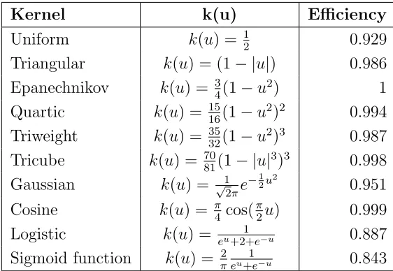
Kernel smoothers are many but the selected kernel should be easy to implement both theoretically and practically. Silverman (1986) gave the following requirements that ought to be met by the smoother.

ii) The kernel smoother should not take very small values that may result in numerical underflow in the computer.

iii) The kernel smoother should be user friendly i.e it should practically fit in both simulated and raw data.

iv) The range of the smoother should be well defined and not open as in the case of Gaussian kernel.

Table 2.1 gives the efficiency of various kernels with respect to the Epanechnkov kernel.

Table 2.1: Efficiency Relative to Epanechnkov Kernel

Kernel k(u) Efficiency

Uniform k(u) = 1₂ 0.929 Triangular k(u) = (1− |u|) 0.986 Epanechnikov k(u) = 3₄(1−u2_{) 1}

Quartic k(u) = 15₁₆(1−u2₎2 _0.994

Triweight k(u) = 35₃₂(1−u2₎3 _0.987

Tricube k(u) = 70₈₁(1− |u|3₎3 _0.998

Gaussian k(u) = √1

2πe

−1

2u2 0.951

Cosine k(u) = π₄ cos(π₂u) 0.999 Logistic k(u) = _eu₊₂₊1 _e−u 0.887

Sigmoid function k(u) = _π2_eu₊1_e−u 0.843

2.2

Existing estimators of the population variance

and their asymptotic properties

Assuming a population consisting of N distinct units of values (xi, yi), and xi > 0 for1 < i < N. Take from the population a SRSWR of size n. The sample and population means ofyi andxiare denoted by ¯yand ¯xrespectively. The ratio estimator

ˆ ¯

YR= ¯YX/¯ x¯ (2.13)

correlated. Royall (1970) proved that the ratio estimator is the BLUE predictor under the following super population model.

Yi =βxi+ei (2.14)

where ei are iid with mean zero and varianceσ2(xi).

There is no closed form for MSE ( ˆy¯R) or Var ( ˆy¯R). Cochran (1977) gave an approximation of Vo and V2 as,

Vo = 1−f

n

1

N −1Σ N

1 ((yi− ¯

Y

¯

X)xi)

2

(2.15)

V2 =

1−f n ( ¯ X ¯ x) 2 1

n−1Σ N

1 ((yi− ¯

Y

¯

X)xi)

2 _(2.16)

Priestly-Chao estimator is given as ˆ

mc(xj) = 1

nhΣiesWi(Xj)yi

where Wi(xj) = ( xi−xi−1

h )K( xi−xj

h )

The smoothing function however has a shortcoming when one needs to extrapolate various values of the survey variable. Furthermore, unlike the usual weighting scheme where the weights sum to one, this particular case the sum of the weights is not equal to one but is rather an approximation. Moreover this estimator assumes that the data set is ordered such that xi−1 < xi and the weights are only applicable to instances where the auxiliary variable is restricted to some interval.

Royall and Eberhardt (1975) suggested the variance estimator given by

VH =V0

¯

xcX¯ ¯

x2₍₁₋ cx2

n )

−1 (2.17)

where ¯xc is the mean of non-sampled units,cx is the x sample coefficient of variation.

VH is approximately unbiased for more general variance patterns and is asymptotically equivalent to Vj.

Another variance estimator, which parameter follows from standard least squares theory, is

VL =

(1−f)

n x¯cX¯

1

n−1Σe 2

i/xi

Cochran (1977) showed that Var ¯ycan be approximated by the approximate vari-ance

V appr= (1−f)

n(N −1)Σ(yi−rx¯)

2

(2.19) where f = n/N and r = ¯y/x¯. For large samples the approximation is adequate. Cochran (1977) showed that for a sample of size (n < 12) Vappr can greatly under-estimate MSE.

Later Royall and Cumberland (1981) suggested a closely related estimator

VD =

(1−f)

n

¯

xcx¯ ¯ x2 1 nΣ ˆ e2 i 1− xi

nx¯

(2.20)

Here bothVH and VD were shown to be unbiased under the model and approximately unbiased for more general variance patterns and asymptotically equivalent to Vj.

Gasser and Muller (1979) proposed an estimator that involved sorting of X vari-able. The estimator is given as

ˆ

mx = Σnj=1

Z sj

sj−1

k(u−1)dusj

where sj = 1₂(xj+xj+1) =−∞ and xn=1 =∞.

The resulting nonparametric estimator of the population variance is given as ˆ

TG = Σiesyi+ Σjermˆ(xj)

Where g(x) is a curve restricted to the functional form. The distance can be reduced by using any g(x) that is used to interpolate the data. This technique yields good results because it produces a good fit and the curve does not have too much variation. Dickey and Fuller (1981) suggested a regression adjustment to V0. The estimator

due to Fuller (1981) is given by

Vreg =V0+

(1−f)

n

ˆ_be2

x( ¯X−x¯) (2.21) where ˆbe2_x is the sample regression coefficient of eˆi

xi.

A common variance estimator is the Jackknife variance estimator Vj,

Vj = (1−f)¯x2

n

(n−1)ΣD

2

j (2.22)

whereDj is the difference between the ratio

(ny¯−yj)

The jackknife estimator is independent of a superpopulation model.

Royall and Cumberland (1981) studied the model-based and sampling properties of Vj and deduced that it is approximately unbiased.

Wu (1982) proposed a general class of estimators V g = gV0, where V0 is the

sample mean of e2_i. It was shown that the first terms of MSE (Vg) is minimized by

gopt =SxzX/S¯ x2Z¯ which is the population regression coefficient of Zi/z¯

Xi/¯x.

Where gopt is the sample regression coefficient of z_z¯i over x_x¯i,Zi =e2i −2eiΣxiei/ΣXi.

S_x2 and Sxz are the population variance and covariance respectively. The second term of Zi accounts for the possible non zero intercept in the population when fitted by a straight line.

Isaki (1983) proposed ratio type estimator of the population varianceS2

y when the population varianceS2

x of the auxiliary variable X is known together with its bias and mean squared error as:

ˆ

S_R2 =S_y2S

2

x

s2

x

(2.23)

B( ˆS_R2) = γS_y2[(β2x−1)−(λ22−1)] (2.24)

M SE( ˆS_R2) =γS_y4[(β2y −1) + (β2x−1)−2]−2(λ22−1) (2.25) where β2y = µ_µ40₂₀,β2x = µ_µ04₀₂,λ22 = _µ20µ22_µ02

When deriving the asymptotic properties of the Nadraya-Watson estimator, it becomes tedious to find the derivatives of the estimator due to the nature of the denominator of the estimator. Otieno and Mwalili(2000) therefore gave the estimator of the finite population variance as

ˆ

Tc = Σiesyi+ Σjermˆc(xj)

The residual sum of squares can be used to compute the regression function. It is given as,

ˆ

ms(xj) = Σn_i=1(yi−g(xi))2

Breidt and Opsomer (2000) studied the Horvitz Thompson estimator of the pop-ulation given by ˆty = Σiesy_πi

i whereπ is the inclusion probability. Breidt and Opsomer

of survey values in the finite population and a matrix of dimensionN∗(q+ 1) defined

byXUi =

       

1 (x1−xi) . . . (x1 −xi)q 1 (x2−xi) . . . (x2 −xi)q

..

. ... . .. ... 1 (xN −xi) . . . (xN −xi)q

       

Define an N∗N matrix byWUi =diag{

1

hNK(

xj−xi

hN )}.ei being a vector of 1 line in

the first position and 0 otherwise. The estimator of the regression function at m(xi) is then given by;

mi =e

0

i(X

0

UiWUiXUi)

−1_(X0

UiWUiXUi) (2.26)

as long as (X_U0

iWUiXUi) is invertible. The design unbiased estimator of the population

variance is then given by

t∗_y = Σies

yi−mi

πi

+ ΣieUNmi (2.27)

which is a generalised difference estimator with variance given by

Vp(t∗y) = Σi,jeUN(πi,j −πiπj)

yi−mi

πi

yj−mj

πj

(2.28)

However, the estimator is based on the entire population. The sample based consistent estimator of the regression function m(xi) is given by;

ˆ

mi =e

0

i(X

0

UiWUiX

−1

Ui )X

0

UiWUiXUi (2.29)

For observations less than (q+ 1), the matrix X_U0_iWUiXUi is singular. Breidt and

Opasomer (2000) therefore considered an adjusted sample based estimator that is guaranteed to exist for any sample drawn from the population. The sample based estimator of the population total is a linear combination of survey values with weights being the inverse inclusion probabilities. The estimator that uses the adjusted sample smoother was found to be asymptotically design unbiased and design consistent. The variance of the estimator was also found to be design unbiased and design consis-tent for the asymptotic mean squared error. The estimator satisfied the property of asymptotic normality and was found to be robust in the sense that it achieved the Godambe-Joshi lower bound.

Upadhyaya and Singh (2001) suggested a modified ratio type variance estimator using the population mean of the auxiliary variable together with its bias and mean squared error as,

ˆ

S₅₂2 =s2_y[ ¯

X

¯

x] (2.30)

M SE( ˆS₅₂2 ) =γS_y4[(β2y−1) +Cx2 −2λ21Cx] (2.32) The proposed variance estimators above are biased but have smaller mean squared errors compared to the traditional ratio type variance estimator suggested by Isaki (1983) under certain conditions.

Zheng and Little (2003) gave the spline estimator of the population variance as ˆ

TC = Σiesyi+ Σjermˆs(xj)

Subramani and Kumarapandiyan (2015) proposed a class of modified ratio type variance estimators ˆS_p2_i for estimating the population variance S_y2 given as

ˆ

S_p2_i =s2_y[ ¯

X+wi ¯

x+wi

], i= 1,2,3, ...,51 (2.33)

Subramani and Kumarapandiyan (2015) derived the bias and MSE of ˆS_p2_i as

Bias( ˆS_p2

i) =

(1−f)

n S

2

y(O

2

piC

2

x−Opiλ21Cx) (2.34)

M SE( ˆS_p2

i) =

(1−f)

n S

4

y((β2(y)−1) +O2piC

2

x−2Opiλ21Cx);i= 1,2,3, ...,51 (2.35)

2.3

Comparison of the relative efficiency of

exist-ing variance estimators

Based on the empirical study by Wu and Deng (1982), the estimator Vo is the least efficient among the estimators that they studied. It has unreliable t-intervals that neither estimates the MSE nor the conditional MSE ofYRwell. However it is the most commonly recommended estimator on sampling. Wu and Deng (1982) showed that the performance of the variance estimatorsVo and V2 for estimating MSE depends on

the underlying populations and has no direct bearing on the performance of interval estimates.

The jackknife variance VJ gives very reliable t-intervals than VH and VD. All the three estimators give t-intervals that are close to V2 for large samples, but not to Vg.

Wu and Deng (1982) emphasized that the reliable t-intervals seems to be related to the good performance of V2 for estimating the conditional MSE. The problem

of choosing a proper ancillary statistic and making inference conditional on it is an important one in the theory of survey sampling. Encouraged by the relative efficiency of V2 over V0, Wu and Deng (1982) considered the variance estimation problem in

other settings.

Otieno and Mwalili (2000) studied the empirical properties of VL, VD,VC and Vn in a natural population. Otieno and Mwalili (2000) found out that one can useVn to estimate the MSE. Otieno and Mwalili (2000) further investigated how efficient the four variance estimators were on tracking the conditional MSE. In the study VD and

Vn both follow the MSE very closely but, VC and VL does not efficiently approximate the MSE.This indicates that Vn is a strong competitor to VD.

The performance of the estimator proposed by Breidt and Opsomer (2000) was compared to that of other parametric and nonparametric estimators. Both the para-metric and nonparametic regression estimators performed better than the Horvitz Thompson estimator. However, the local polynomial regression estimator by Breidt and Opsomer (2000) was the best estimator among the nonparametric estimators considered.

2.4

Research Gap

Chapter 3

Research Methodology

3.1

Introduction

This chapter presents the estimation of variance, the variance of the ratio estimator under robust variance structure of the population mean, multiplicative bias robust variance estimator for ratio estimator using a smoother function and the asymptotic properties of the multiplicative bias corrected variance estimator.

3.2

Estimation of Variance

Estimation of variance is taken in consideration in this study. Suppose that there are units U1, U2, ..., UN with corresponding survey measurements y1, y2, ..., yN for the survey variable Y. If all the units are labeled and supposing that in each unit it is possible to collect survey measurements, then it is possible to determine variance for any set of data collected.

3.3

The variance of the ratio estimator under

ro-bust variance structure of the population mean

In this section, the exact procedure of estimating the robust variance of the population mean is presented. Let u = (u1, ..., uN) be a finite population of size N < ∞. Suppose that for every unitui, some unknown measurement (auxiliary measurement) denoted asxi;(i=1,2, , N) exists. It is of interest to find an estimator of the population variance i.e.

Y =µ(xi) +ei

E(y) = µ(xi)

Cov(Yi, Yj) =σ2(xi), f ori=j,0otherwise

whereµ(xi) andσ2(xi) are assumed to be smooth functions of xi mainly because the above are the simplest form of equations that describes the relationship between the auxiliary variable and the survey variable.

A simple random sample of size n is taken from the population U. The problem is how to estimate T, using knownxi, s in the entire population and the sampled values of yi ’s.

It is a common practice in survey sampling to use a ratio estimator in such context, especially when there is positive correlation between the auxiliary measurementsxi’s and the survey measurementsyi’ s.

Let ¯x,¯y be sample means of xi’s , yi ’s respectively and ˆX and ˆY be the corre-sponding population values. Then the estimator:

ˆ

TR= ¯

yX¯

¯

x =rn

¯

X (3.2)

where rn= y_¯x¯. ˆTR is called the ratio estimator of the population mean ˆY. A ratio estimator of the population is given by

ˆ

T =Ny¯

¯

x

¯

X =N rnX¯

The ratio estimator is generally motivated on the basis of a [superpopulation model, prediction model]. The ratio estimator is BLUE under the above model (best linear unbiased estimator). An estimator ˆθ is said to be model unbiased under the model if

Ecs(ˆθ) =Ecs(θ). that is under the above model if

Ecs( ˆTR) =Ecs(rnX¯)

Ecs(rnX¯ = ¯XEcs(rn) = ¯

X

¯

xEcs(¯y)

= ¯ X ¯ x 1 nΣ n

i=1E(yi) =βX¯

ButEcs( ¯Y) = Ecs 1

nΣ

n

i=1yi =βX¯ ˆ

TR is model unbiased estimator of the population mean, ¯Y. Then clearly,

Ecs( ˆTR−T) =Ecs( ˆTR−Yˆ) =

α ¯ x( ¯ X ¯

x) = αx¯

¯

which is not equal to zero.

Clearly R is not bias robust to model misspecification: E(Y i) =α+βxi.Many studies prefer using a ratio estimator R of the population mean ˆY in the presence of auxiliary measurements xis, (i= 1, ..., N). In such studies it is believed that the regression line passes through the origin. Assuming this to be true,this project is concerned with estimating the precision of the ratio estimator when the variance function is not linearly related to the auxiliary measurement xi (i = 1,2, ..., N). In particular we consider the following model Ecs(Yi) =βxi

The robust model of the variance of yi’s is given by

cov(Yi, Yj) =σ2(xi) =j 0, i6= 0

The function σ2_(x

i) is assumed to be twice continuously differentiable. Under the above model,

ˆ

TR−T = (Σiesyi+rΣierxi)−(Σiesyi+rΣieryi) (3.3) =rΣierxi−Σieryi

= Σsyi( Σrxi Σsxi

)−Σryi

V ar( ˆTR) = ( Σrxi Σsxi

)2Σsσ2(xi) + Σrσ2(xi) (3.4) then,

V ar( ˆTR) = ( Σrxi Σsxi

)2Σiesσ2xi+ Σierσ2xi =σ2Σierxi[Σierxi

Σiesxi + 1]

=σ2Σierxi(

Σrxi+ Σsxi Σsxi

)

(N(N−n) ¯Xx¯r

nx¯s

)σ2

A number of parametric estimators for estimating V ar( ˆTR) as studied by Otieno and Mwalili (2000) include:

VC =

N2(1−f)

n [Σies

ˆ

e2_i

(n−1)]

VL=

N2_(1−f)

n2

¯

XX¯r ¯

x2 Σies

ˆ

e2

i

√

VN = Σjeswj2(Xi)ˆσnp2 (xi) + Σjerσˆ2np(xi)

Where f = _Nn ,ˆei = yi − _xy_¯¯s_sxi,¯ys is the sample mean of yi0s, ¯Xr, ¯xs represent non-sample and sample means of x0_is respectively. Moreover, ˆσ_np2 = Σjeswj(xi)ˆe2j and

wj(x) is a weight.

In the recent past a non-parametric variance estimator based on Nadaraya-Watson smoother has been proposed. This estimator is based on squared residuals

e2_i = (yi−rxi)2

The estimator of equation (3.4) is then obtained by substituting a smoother toσ2_(x

i) in (3.4) as

ˆ

σ2(xi) = Σjeswj(xi)ˆe2j to give,

VN w = ( Σrxi Σs(xi

)2ΣiesσˆN w2 (xi) + ΣierσˆN w2 (xi) (3.5) here wj(xi) = 1₄(1−u2i). This estimator, like many other Kernel smoothers suffers from boundary problem, including outlier sensitivity.

In this project a multiplicative bias reduction procedure is used to develop a bias robust variance estimator.

3.4

Multiplicative bias robust variance estimator

for ratio estimator using a smoother function

Suppose (X1, Y1),(X2, Y2)...,(XN, YN) are bivariate independent r.vs (X, Y). As-sume allXi’s are unknown.

Define

ˆ

e2

j =σ2(Xi) +O(n−1) = σ2(Xi) +i (3.6) Consider a smoother of variance function

σ_n2(Xi) = ΣjesWj(Xi)ˆe2j (3.7) Then the ratio βj = _σ2e₍j_X

i) is a noisy estimator of

σ2_(X i)

σ2 n(Xi.

Smoothing βj yields

ˆ

α(Xi) =σn2(Xi)βj (3.8) Equation(3.8) is used as a multiplicative correction of the pilot smoother in equa-tion (3.7) and is defined as

ˆ

Assumptions of the study

The following assumptions are made in the estimation of ˆσ2

n(Xi) a)The regression function is bounded and strictly positive i.e

b)0 < a < σ(xi)< b

c)The regression function is twice continuously differentiable everywhere.

The positivity assumption on the regression function σ(xi) is important when performing the multiplicative bias correction.The regression function might cross the x-axis and in such a situation Glad (1998) proposed to shift all the response data by a distance a such that the new regression function is σ(xi) +a

substituting (3.8)to (3.9) yields,

ˆ

σn(xi) = Σn_j=1wj(xi) ˆ

σn(x) ˆ

σnxj

yj (3.10)

Suppose that

E[ˆσ(x)|xi, ..., xN] = Σnj=1wj(xi)E[Yj] = Σnj=1wj(xi)σ(Xj) = ˆσn(x) (3.11) Using σˆn(x)

ˆ

σnxj in equation (3.10)yields

ˆ

σn(x) ˆ

σnxj

= σ¯n(x) ¯

σnxj

∗ σˆn(x)

ˆ

σn(xj)

∗(σˆn(xj) ˆ

σnxj

)−1 (3.12)

ˆ

σn(x) ˆ

σn(xj)

= σ¯n(x) ¯

σn(xj)

∗(σ¯n(x) + ˆσn(x)−σ¯n(x) ¯

σn(x)

)∗(

¯

σ(xj) ¯

σ(xj) + ˆσ(xj)−σ¯(xj)

) (3.13) ˆ

σn(x) ˆ

σn(xj)

= σ¯n(x) ¯

σn(xj)

∗(1 + σ¯n(x)−_¯ σ¯n(x)

σn(x)

)∗(1 + σˆn(xj)−σ¯(xj) ¯

σ(xj)

)−1 (3.14) Let σ¯n(x)−σ¯n(x)

¯

σn(x) ) =bn(x) and

ˆ

σn(xj)−σ¯(xj)

¯

σ(xj) =bn(xj).

Equation (3.14)can now be expressed as, ˆ

σn(x) ˆ

σn(xj)

= σ¯n(x) ¯

σn(xj)

∗(1 +bn(x))∗(1 +bn(xj))−1 (3.15) Applying the binomial expansion to equation (3.15) yields

This further reduces to

(1 +bn(x))∗(1 +bn(xj))−1+rj(x, xj) = 1 +bn(x)−bn(xj) +rj(x, Xj) (3.16) whererj(x, xj) is the remainder term involvingxand xj Substituting equation (3.16) to equation (3.15) yields

ˆ

σn(x) ˆ

σn(xj)

= σ¯n(x) ¯

σn(xj)

∗[1 +bn(x)−bn(xj) +rj(x, xj)] (3.17)

Substituting equation (3.17) to equation (3.10)and using the model Yj =σ(Xj) +ej yields,

ˆ

σn(Xi) = Σnj=1wj( ¯

σn(x) ¯

σn(xj)

∗[1 +bn(x)−bn(xj) +rj(x, xj)][σ(Xj) +ej]) (3.18)

ˆ

σn(Xi) = Σnj=1wj(( ¯

σn(x) ¯

σn(xj)

σ(Xj)∗[1 +bn(x)−bn(xj) +rj(x, xj)])

+Σn_j=1wj(( ¯

σn(x) ¯

σn(xj)

ej[1 +bn(x)−bn(xj) +rj(x, xj)]) (3.19)

ˆ

σn(Xi) = Σnj=1wj ¯

σn(x) ¯

σnxj

σ(Xj)+Σnj=1wj ¯

σn(x) ¯

σnxj

(ej+σ(Xj)[bn(x)−bn(xj)])+Σnj=1wj ¯

σn(x) ¯

σnxj

ej (3.20) [bn(x)−bn(xj) +rj(x, xj)] + Σnj=1wj

¯

σn(x) ¯

σnxj

rj(x, xj)[σ(Xj) +ej] (3.21) Applying the assumption thatnh→ ∞, in probability the remainder terms converge to 0. Thereforerj(x, xj)[σ(Xj) +ej] =Op(_nh1 ) and equation (3.20)reduces to,

ˆ

σn(Xi) = Σnj=1wj ¯

σn(x) ¯

σnxj

σ(Xj)+Σnj=1wj ¯

σn(x) ¯

σnxj

(ej+σ(Xj)[bn(x)−bn(xj)])+Σnj=1wj ¯

σn(x) ¯

σnxj

ej

[bn(x)−bn(xj) +rj(x, xj)] +Op( 1

nh) (3.22)

Our estimator of the population variance therefore is

ˆ

VM BC = ΣiesYi+ Σie(p−s)[Σnj=1wj(x;h) ˆ

σn(x) ˆ

σn(xj)

+ Σn_j=1wj(x;h) ˆ

σn(x) ˆ

σn(xj) (ej

σ(xj)[bn(x)−bn(xj)]) + Σnj=1wj(x;h) ˆ

σn(x) ˆ

σn(xj)

ej[bn(x)−bn(xj)] +Op( 1

3.5

Asymptotic Unbiasedness of the MBC

Estima-tor

Under the model based approach, the bias of the estimator ˆVM BC is defined by,

E[ ˆVM BC−V] =E[ ˆVM BC]−E[V] The expected value of the MBC estimator is calculated as,

E[ ˆVM BC] =E[ΣiesYi+ Σje(p−s)(Σnj=1σˆn(xi))] = ΣiesE[Yi] + Σie(p−s)Σn

j=1E[ˆσn(xi)] (3.24)

The calculation of E[ˆσn(xi)] is based on establishing a stochastic approximation of the estimator ˆσn(xi) in which each term can be directly analyzed.

E[ˆσn(xi)] = E[Σnj=1wj(x;h) ˆ

σn(x) ˆ

σn(xj)

σ(xj)+Σnj=1wj(x;h) ˆ

σn(x) ˆ

σn(xj)

(ej+σ(Xj)[bn(x)−bn(xj)])

+Σn_j=1wj(x;h) ˆ

σn(x) ˆ

σn(xj)

ej(bn(x)−bn(xj)) +Op( 1

nh)] (3.25)

=E[Σn_j=1wj(x;h) ˆ

σn(x) ˆ

σn(xj)

σ(xj) + Σnj=1wj(x;h)Aj(x) + Σnj=1wj(x;h)Bj(x)] +Op( 1

nh)

(3.26) Where

Aj(x) = ¯

σn(x) ¯

σnxj

(ej+σ(Xj)[bn(x)−bn(xj)]) and

Bj(x) = ¯

σn(x) ¯

σnxj

ej[bn(x)−bn(xj)] Analyzing the first term of equation (3.26)

E[Σn_j=1wj(x;h) ˆ

σn(x) ˆ

σn(xj)

σ(xj)]

yields

Σn_j=1wj(x;h) ˆ

σn(x) ˆ

σn(xj)

σ(xj)

E[Σn_j=1wj(x;h) ˆ

σn(x) ˆ

σn(xj)

(ej+σ(Xj)[bn(x)−bn(xj)])]

=E[Σn_j=1wj(x;h)] (3.27) This yields

E[Σn_j=1wj(x;h) ¯

σn(x) ¯

σn(xj)

] = Σn_j=1wj(x;h) ¯

σn(x) ¯

σn(xj)

This is becauseσ(Xj) is the variance function. Analyzing the second term of equation (3.26)

E[Σn_j=1wj(x;h) ¯

σn(x) ¯

σn(xj)

(ej +σ(Xj)((bn)(x)−bn(Xj))]

=E[Σn_j=1wj(x;h)( ¯

σn(x) ¯

σn(xj)ej+ ¯

σn(x) ¯

σn(xj)

σ(Xj)( ¯

σn(x)−σ¯n(x) ¯

σn(x) )− ¯

σn(x) ¯

σn(xj)

σ(Xj)( ¯

σn(xj)−σ¯n(xj) ¯

σn(xj) )] = Σn_j=1wj(x;h)

¯

σn(x) ¯

σn(xj)

E[ej]+Σnj=1wj(x;h) ¯

σn(x) ¯

σn(xj)

E[ej]−Σjn=1wj(x;h) ¯

σn(x)σ(xj) ¯

σ(Xj)2

E[¯σn(Xj)]

+Σn_j=1wj(x;h)E[¯σn(x)σ(xj) ¯

σ(Xj)

] (3.29)

[Σn_j=1wj(x;h) ¯

σn(x) ¯

σn(xj)

(ej+σ(Xj)((bn)(x)−bn(Xj))] = 0+0−Σnj=1wj(x;h) ¯

σn(x)σn(Xj)¯σ(Xj) ¯

σ(Xj)2 +Σn_j=1wj(x;h)

¯

σn(x)σn(Xj) ¯

σ(Xj)

E[1] (3.30)

E[Σn_j=1wj(x;h) ¯

σn(x) ¯

σn(xj)

(ej +σ(Xj)((bn)(x)−bn(Xj))]

= 0 + 0−Σn_j=1wj(x;h) ¯

σn(x)σn(Xj) ¯

σ(Xj)

+ Σn_j=1wj(x;h) ¯

σn(x)σn(Xj) ¯

σ(Xj)

(3.31) Thus

E[Σn_j=1wj(x;h) ¯

σn(x) ¯

σn(xj)

(ej +σ(Xj)((bn)(x)−bn(Xj))] = 0 (3.32) Analyzing the third term of equation (3.26)

E[Σn_j=1wj(x;h) ¯

σn(x) ¯

σn(xj)

ej((bn)(x)−bn(Xj))] =

E(Σn_j=1wj(x;h)[ ¯

σn(x) ¯

σn(xj)

ej ¯

σn(x)−σ¯n(x) ¯

σn(x)

]− σ¯n(x)

¯

σn(xj)

ej( ¯

σn(xj)−σ¯(xj) ¯

σn(xj)

)] (3.33)

E[Σn_j=1wj(x;h) ¯

σn(x) ¯

σn(xj)

ej((bn)(x)−bn(Xj))] =

Σn_j=1wj(x;h) ¯

σn(x) ¯

σn(xj)

[σ¯n(x)−σ¯n(x) ¯

σn(x)

]E[ej]−Σjn=1wj(x;h) ¯

σn(x) ¯

σn(xj)

[¯σn(xj)−σ¯n(xj) ¯

σn(xj)

]E[ej] (3.34) Therefore

E[Σn_j=1wj(x;h) ¯

σn(x) ¯

σn(xj)ej((bn)(x)−bn(Xj))] = 0 (3.35) equation (3.26)thus reduces to

E[ˆσn(xi)] = Σjn=1wj(x;h) ¯

σn(x) ¯

σn(xj)

σ(Xj) +Op( 1

ThusE[ ˆVM BC] is given by the expression

E[ ˆVM BC] = ΣiesY¯i+ Σie(p−s)[Σnj=1wj(x;h) ¯

σn(x) ¯

σn(xj)

σ(Xj)] +Op( 1

nh) (3.37)

Equation (3.36) can be simplified by taking a Taylor series expansion of the ratio

¯

σn(x)

¯

σn(xj) about the point xas follows.

¯

σn(x) ¯

σn(xj) = ¯

σn(x) ¯

σn(xj)

+ (Xj−x)(

σ(x) ¯

σn(x))

0

+ 1

2(Xj −x)

2₍σ(x)

¯

σn(x))

00

+ (1 +Op) (3.38)

Substituting equation (3.38) to equation (3.37) yields

E[ ˆVM BC] = ΣiesY¯i+ Σie(p−s)[Σnj=1wj(x;h)¯σn(x)(

σ(x) ¯

σn(x)

+ (Xj−x)(

σ(x) ¯

σn(x) )0

+1

2(Xj −x)

2 σ(x)

¯

σn(x)

)00+ (1 +Op))] +Op( 1

nh) (3.39)

Considering the first two terms of the Taylor series expansion,equation (3.39) reduces to

E[ ˆVM BC] = ΣiesY¯i+ Σie(p−s)[Σnj=1wj(x;h)ˆσn(x)(

σ(x) ˆ

σn(x)

+ (Xj −x)(

σ(x) ˆ

σn(x)

0

)] +Op( 1

nh)

(3.40) since Σn_j=1wj(x;h) = 1 and Σnj=1wj(x;h)(Xj−x) = 0,equation (3.40)can be expressed as

E[ ˆVM BC] = ΣiesY¯i+ Σie(p−s)[Σnj=1wj(x;h)σ(x)] +Op( 1

nh) (3.41)

Also we have,

T = ΣiesYi+ Σie(p−s)Yi (3.42)

E[T] =E[ΣiesYi+ Σie(p−s)Yi] (3.43) Substituting equation (3.41) and equation (3.43) into equation (3.23)yields,

E[ ˆVM BC−T] = ΣiesYi+ Σie(p−s)[Σnj=1wj(x;hσ(x)] +Op( 1

nh)−[ΣiesYi+ Σie(p−s)σ(x)]

(3.44)

E[ ˆVM BC−T] = Σie(p−s)[Σnj=1wj(x;h)σ(x)]−Σie(p−s)σ(x) +Op( 1

nh) (3.45)

Hence the bias of ˆVM BC is given by;

Bias[ ˆ

VM BC

N ] =E[

ˆ

VM BC−T

N ] =

1

N[Σie(p−s)Σ

n

j=1(wj(x;h)σ(x))−Σie(p−s)σ(x)]+Op( 1

nh)

3.6

Asymptotic Variance of the MBC estimator

Using equation (3.21),the estimator of the robust variance is given by; ˆ

VM BC = ΣiesYi+ Σie(p−s)[Σnj=1wj(x;h) ˆ

σn(x) ˆ

σn(xj) + Σ n

j=1wj(x;h) ˆ

σn(x) ˆ

σn(xj)(ej

σ(xj)[bn(x)−bn(xj)]) + Σnj=1wj(x;h) ˆ

σn(x) ˆ

σn(xj)ej[bn(x)−bn(xj)] +rj(x, Xj) (3.47) where rj(x, Xj) is the remainder term that involves the terms x and Xj using the assumption that nh → ∞,the terms converge to zero in probability. Therefore

rj(x, Xj)[σ(Xj) +ej] =Op(_nh1 ) and equation (3.47) reduces to ˆ

VM BC = ΣiesYi+Σie(p−s)[Σnj=1wj(x;h) ˆ

σn(x) ˆ

σn(xj)

∗[ˆσn(xj)+ej][1+bn(x)−bn(xj)]+Op( 1

nh)

(3.48) Truncating the binomial expansion at the first term yields

ˆ

VM BC = ΣiesYi+ Σie(p−s)[Σnj=1wj(x;h) ˆ

σn(x) ˆ

σn(xj)

∗[ˆσn(xj) +ej] +Op( 1

nh) (3.49)

The variance of the estimator is then defined by;

V ar[ ˆVM BC] =V ar[ΣiesYi+ Σie(p−s)[Σnj=1wj(x;h) ˆ

σn(x) ˆ

σn(xj)

∗[ˆσn(xj) +ej] +Op( 1

nh)]

(3.50) =V ar[ΣiesYi]+V ar[ΣiesYi]+V ar[Σie(p−s)[Σnj=1wj(x;h)

ˆ

σn(x) ˆ

σn(xj)

∗[ˆσn(xj)+ej]+(Op( 1

nh))

2

(3.51)

V ar[ ˆVM BC] =V ar[ΣiesYi] + [Σie(p−s)Σnj=1wj(x;h) ˆ

σn(x) ˆ

σn(xj)

∗V ar(Yj)] + (Op( 1

nh))

2

(3.52)

V ar[ ˆVM BC] = Σiesσ2(xi) + Σie(p−s)Σnj=1(wj(x;h))2( ˆ

σn(x) ˆ

σn(xj)

)2σ2(xi) +Op( 1

nh))

2 _(3.53)

Obtaining the Taylor series expansion of the ratio σ2(xj)

σ(xj)2 in the second part of the

equation (3.53) gives

V ar[ ˆVM BC] = Σiesσ2(xi) + Σie(p−s)Σjn=1(wj(x;h))2σ2(xi) +Op( 1

nh))

2

(3.54)

Thus the asymptotic variance of [VˆM BC

N ] is given by;

V ar[VˆM BC

N ] =

1

N2Σiesσ 2_(x

i) + 1

N2Σie(p−s)Σ

n

j=1(wj(x;h))2σ2(xi+Op( 1

nh))

3.7

Asymptotic Mean squared of the MBC

esti-mator

The mean squared error of ˆVM BC is given by

M SE[ ˆVM BC] =V ar[ ˆ

VM BC

N ] + [Bias[

ˆ

VM BC

N ]

2_{] (3.56)}

Bias[VˆM BC

N ] =E[

ˆ

VM BC −T

N ] =Op(

1

nh) (3.57)

using equation (3.55) and (3.57) in equation (3.56) yields

M SE[ ˆVM BC] = 1

N2[Σiesσ 2

(xi) + Σie(p−s)Σnj=1(wj(x;h)) 2

σ2(xi)] +Op( 1

nh))

2

Chapter 4

Empirical Study

4.1

Introduction

This chapter presents the description of the population and the results of the asym-potic variance estimators.

4.2

Simulation Procedure

A simulation experiment is performed in order to investigate the statistical proper-ties of the proposed estimator as well as compare its performance to that studied by Otieno and Mwalili (2000). The unconditional MSE and Biases are computed for each of the variance estimators. R statistical programming version R.2.12.1 is employed to simulate the coverage probabilities using randomly selected samples of size n=50, n=100, n=200, n=500 and n=1000. The samples of n=50, n=100, n=200, n=500 and n=1000 are generated using simple random sampling without replace-ment. A comparison of the performance of the proposed estimator and the variance estimators studied by Otieno and Mwalili (2000) over the randomly selected samples is done. The biases of the proposed variance estimator and those studied by Otieno and Mwalili (2000) are calculated. The Root Mean squared Error(RMSE) for the proposed variance estimators is calculated as given below,

RM SE(VM BC) =

s

1

N( ˆVM BC −T)

2

The results are displayed in a table and was compared to the following rival estimators,

RM SE(VN) =

s

1

N( ˆVN −T)

2

RM SE(VC) =

s

1

N( ˆVC −T)

RM SE(VL) =

s

1

N( ˆVL−T)

2

4.3

Simulation Results

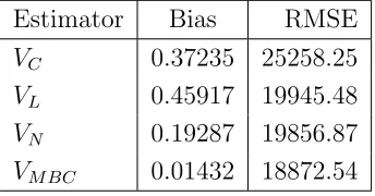
Table 4.1 represents the unconditional biases and root Mean Squared Errors (RMSE) for the multiplicative bias corrected estimator and those studied by Otieno and Mwalili (2000). Table 4.1 show that the bias and the RMSE of the multiplicative bias corrected estimator is lower than the bias and mean squared error of the vari-ance estiamtors studied by Otieno and Mwalili(2000).

Table 4.1: Unconditional biases and RMSE from simulated data Estimator Bias RMSE

VC 0.37235 25258.25

VL 0.45917 19945.48

VN 0.19287 19856.87

VM BC 0.01432 18872.54

Table 4.2 gives a comparison of the coverage probabilities of the four variance esti-mators for different population sizes. The coverage probabilities for the Multiplicative bias corrected estimator is closer to the nominal value of 0.95 than are the coverage probabilities for the other three rival variance estimators. The variance estimatorVL has a better coverage ability under a small sample size of n=50.

Table 4.2: Summary of the unconditional coverage probabilities from the simulted data.

4.4

Real data analysis of the population

A population of size 188 was obtained from United Nations development Programme 2015. UN studied development in 188 countries. UN grouped development in the countries as either very high human development, high human development, medium human development or low human development. Kenya tops the list in countries under low medium development as per the UN statistics 2015 and ranks at number 145 among the 188 countries studied. The UN study used Human Development Index (HDI), Life expectancy at birth, Expected years of schooling, Mean years of schooling, Gross National Income (GNI) per capita and GNI per capita rank minus HDI to rank human development index in the 188 countries.

In this study a relationship between HDI and GNI is considered. HDI acts as the auxiliary variable while GNI acts as the variable under studyyi(i= 1,2,3, ...,188). Figure 4.1 gives a scatter plot of HDI against GNI and also demonstrates a line of best fit between GNI and HDI.

0.4 0.5 0.6 0.7 0.8 0.9

0

20000

60000

100000

SCATTERPLOT

data$HDI

d

a

ta

$

G

N

I

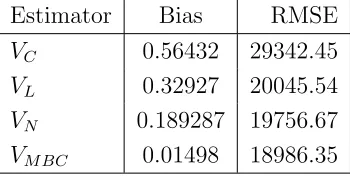
Table 4.3 presents the unconditional biases and RMSE for the multiplicative bias corrected estimator and those studied by Otieno and Mwalili (2000) from the actual data set.

Table 4.3: Unconditional biases and RMSE from actual data Estimator Bias RMSE

VC 0.56432 29342.45

VL 0.32927 20045.54

VN 0.189287 19756.67

VM BC 0.01498 18986.35

Employing R statistical programming version R.2.12.1, simulate the coverage probabilities using randomly selected samples of size n=50, n=100, n=200, n=500 and n=1000 from the UN data. Table 4.4 gives a summary of the results of coverage probabilities using a nominal value of 0.95.

Table 4.4: Summary of the unconditional coverage probabilities from the actual data set

Sample size VM BC VN VL VC n=50 0.912 0.798 0.942 0.832 n=100 0.862 0.763 0.621 0.798 n=200 0.934 0.821 0.451 0.524 n=500 0.962 0.926 0.689 0.653 n=1000 0.949 0.931 0.664 0.792

4.5

Comparison of simulated data and real data

4.6

Conclusion

The main objective of this study was to construct a robust variance estimator of the ratio estimator of the population mean using a multiplicative bias correction technique. As a way of achieving this, a pilot smoother was utilized and the resulting variance estimator using the multiplicative bias correction technique was found to be a useful tool in correcting of boundary bias. The methodology used possesses a kind of robustness in the sense that the multiplicative factor is bounded. The method is easy to implement and has good asymptotic properties both theoretically and practically. We have also assessed the performances of our estimator with that of the existing estimators for simulated data and real data sets. It is observed from the numerical comparison that our proposed estimatorVM BC is more efficient than existing variance estimators. The derived estimatorVM BC has better coverage probability as compared to rival variance estimators of the population mean.

4.7

Recommendation for further study

In this study, a single auxiliary variable was considered. The use of more than one auxiliary variable need to be investigated and the performance of the resulting esti-mator compared to determine if it yields better estimations.

References

Chambers, R.L., Dorfman, A.H.Wehrly, T.E.(1993). Bias robust estimation in finite populations using non parametric calibration. Journal of the American Statistical Association 88 : 268−277.

Cochran, W.G.(1977) Sampling Techniques. Edn. 3. Wiley Eastern Publication, New York.

Hansen, M. H. , Hurwitz, W. N. and Madow, W.O.(1983). An evaluation of model dependent and probability sampling inference in sample surveys. Journal of the American Statistical Association 78:776.-807.

Otieno and Mwalili (2000). Nonparametric regression method for estimating the error variance in unistage sampling. East African Journal of Science 2(2):107-112 (2000).

Nadaraya, E.pt.(1964). On estimating regression. Theory of Probability Applications 9: 141-142.

Royall, R. M.and Cumberland, W.O.(1981). An empirical study of the ratio estimator and estimators of its variance. Journal of the American Statistical Association 76:66-77.

Silverman, (1986). Density Estimation.Chapman and Hall, London.

J.Subramani and G.Kumarapandiyan (2015). A class of ratio estimators for estimation of population variance jamsi, 11 (2015), No.1

Dorfman, A.H. (2009) Nonparametric Regression and the Two Sample Problem. Proceedings of the Joint Statistical Meetings, Section on Survey Research Methods, Washington DC, August 1-6 2009, 277-270.

Quenouille, M. H. (1949). Approximate tests of correlation in time-series. J.R. Statistic. Soc. B 11, 68-84.

Linton, O. and Nielsen, J.P. (1994). A Multiplicative Bias Reduction Method for Nonparametric Regression. Statistics and Probability Letters , 19, 181-187. Dorfman, A.H. (1992) Nonparametric Regression for Estimating Totals in Finite Populations. Proceedings of the Section on Survey Research Methods , American Statistical Association Alexandria, Washington DC, 622-625.

Brewer, K. R. W., Ratio estimation and finite populations: Some results deducible from the assumption of an underlying stochastic process, Australian Journal of Statistics 5 (1963), 93-105.

Wu, C. F., Estimation of variance of the ratio estimator, Biometrika 69 (1982), 183-189.

Isaki, C.T. (1983). Variance estimation using auxiliary information. Journal of the American Statistical Association, 78:117-123.

Upadhyaya, L.N. and Sing, H.P. (2001). Estimation of population standard deviation using auxiliary information. American Journal of Mathematics and Management Sciences, 21(3-4), 345-358.

Royall, R. M. and Eberhardt, K. R. (1975). Variance estimates for the ratio estimator, Sankya, Ser. C 37, 43-52.

Royall, R. M. (1970). On finite population sampling theory under certain linear regression models. Biometrika 57, 377-387.

Krewski, D. ; Rao, J. N. K. (1981). Inference From Stratified Samples: Properties of the Linearization, Jackknife and Balanced Repeated Replication Methods. Ann. Statist no. 5, 1010–1019.

Priestly, M. B. and Chao, M. T. (1972). Non-Parametric Function Fitting. Journal of the Royal Statistical Society, Series B, 34, 385–392.

Appendix I: Multiplicative Bias Correction

Simulation

> data <−read.delim(f ile.choose(), header=T)

> data

xbar=mean(HDI)

xbar

sumy =sum(GN I)

> linearM od <−lm(GN I HDI)

> linearM od <−lm(dataGNI dataHDI)

> print(linearM od)

Call:

lm(f ormula=dataGNI dataHDI)

Coef f icients: (Intercept)dataHDI

> scatter.smooth(x=dataHDI, y=dataGN I, main= ”SCAT T ERP LOT”)

> cor(dataHDI, dataGN I)

Appendix II: Conditional Bias Regression

> n <−50

> data

> mse <−numeric(n)

> bias <−numeric(n)

> f or(iin1 :n)

+mse[i]<−M SE((1−data[i])∗Z, mu) +bias[i]<−mu∗data[i]

+variance[i]<−(1−data[i])2

plot(x, mse, type= ”o”, col= ”blue”, pch= ”o”, lty = 1, ylim=c(0,1000), xlab= ”(Groupmean)/100”, ylab= ”Averagesquaredpredictorerror”, main=

”AverageSquaredP redictorError”)

> lines(x, vc, type= ”o”, col = ”red”, lty = 2)

> lines(x, vl, type= ”o”, col= ”green”, lty = 3)

> lines(x, vn, type= ”o”, col = ”orange”, lty = 4)

> lines(x, vmbc, type= ”o”, col = ”black”, lty = 5)

legend(”bottom”, legend =c(”M SE”,”V C”,”V L”,”V N”,”V M BC”), col=

c(”blue”,”red”,”green”,”orange”,”black”), lty = 1 : 5, cex= 0.8)

Appendix III: Coverage probabilities

N =c(50,100,200,500,1000)

CP =array(0, length(N))

f or(kin1 :length(N)) [n=N[k]

X =array(rexp(n∗1000), c(1000, n))

M =apply(X,1, mean)

M X =apply(X,1, max)

M N =apply(X,1, min)

C = (M X −M N)/(2∗sqrt(n))