Comprehensive Analysis of Shielding Effectiveness of Enclosures
with Apertures: Parametrical Approach
Ibrahim B. Ba¸syi˘git* and Mehmet F. C¸ a˘glar
Abstract—The main section of this paper comprehensively analyzes electrical shielding effectiveness (ESE) of enclosures with rectangular apertures for producing valuable information used in electromagnetic interference and compatibility guiding enclosure designers of electronic devices. Firstly, results of conventional analytical equivalent circuit model, measurement and simulation with computer
simulating technology (CSTTM) of ESE for an enclosure with a single aperture size are compared
to improve closeness in different models at 0–1 GHz. After getting a suitable simulation model, all possible parameters with detailed cases are examined to approach beneficial conclusions. Especially, size of enclosure, aperture size, aperture shape, configuration and number of apertures, probe position parameters that affect ESE are investigated. Also, some double parameters are analyzed together to achieve detailed review as two enclosure dimensions, two aperture dimensions and probe position with enclosure depth. Therefore, three-dimensional graphical investigations are performed. Obtained results of these parametric approaches are explained with acceptable reasons. Finally, detailed and itemized comments are given about simulated results of ESE parameters, which are collected from previous sections.
1. INTRODUCTION
Electromagnetic shielding is usually used to decrease the emissions or to the progress of equipment immunity. By increasing used shielding enclosures for electronics systems, apertures and slots of these
enclosures come into prominence for heat allocation, ventilation, I/O cable, etc. These slots and
apertures induce the coupling route of electromagnetic interference (EMI) from the inside to outside [1]. So, metallic shielding enclosures are generally used to reduce radiation from external electromagnetic fields and exudation effects from interior devices. The general definition of the shielding effectiveness (SE) according to the IEEE Standard 299 (IEEE Standard Method for Measuring the Effectiveness of Electromagnetic Shielding Enclosures) [2] is generally used to determine the efficiency of a shield.
Electrical shielding effectiveness (ESE) can be identified in Eq. (1). Ea and Ep are the electric field
strengths with absence and presence of enclosure, respectively
ESE= 10 log10Ea
Eb [dB] (1)
Robinson et al. [3] claimed an analytical formulation based on a transmission line model, where the rectangular enclosure and aperture are modeled by a short-circuit rectangular waveguide and a coplanar strip transmission line, respectively. There are also many studies on analytical method on ESE of enclosures with apertures: New formulas based on electromagnetic [4–7], circuit models [8–10], transmission line theory [11] and surface equivalent principles [12] are some of the analytical methods
Received 25 July 2016, Accepted 2 October 2016, Scheduled 5 December 2016 * Corresponding author: Ibrahim Bahadir Basyigit ([email protected]).
used to calculate ESE. These analytical methods are common and accurate but can be applied only to very simple geometries with approximations.
There are numeric methods to calculate ESE of enclosures with apertures: Finite difference time domain (FDTD) [13–15], transmission line matrix (TLM) [9, 16], and moment of method (MoM) [17]. These numerical methods are useful for complex apertures of enclosures and also accurate, but lead to high cost, big memory on computer and high CPU time. For example, MoM technique requires thousands of seconds for running per frequency point on computers with high speed (3–4 GHz) and high capacity. So, it takes 3–4 hours to produce data containing nearly one thousand frequency points. Also different transformation codes on numerical methods take more time to get data.
We have already investigated aperture size [18] by measurement results and some parameters of magnetic shielding effectiveness (MSE) [19] by theoretical results before. In this study, computer
simulating technology on electromagnetic compatibility (CSTTM-EMC) based on finite integration
technique (FIT) in time-domain [20] is used to acquire accurate modeling results for comprehensive analysis of ESE of enclosures with apertures in 0–1 GHz in many different viewpoints. It should be noted that some studies calculate ESE of enclosure with apertures using CST microwave simulation [6, 12, 21]. Among studies in literature about SE, only a few analyze cases for some shielding parameters as aperture size, enclosure size, and enclosure depth and probe position. Unlike these studies, in this paper as the first novelty, similar shielding parameters with 18 cases are investigated and analyzed in details with cause and effect relation of electromagnetic principles to get more useful suggestions for designers. As the second novelty, the length and width of apertures, the length and width of enclosures and probe position and enclosure depth are analyzed in cross-evaluation with three-dimensional (3D) figures for selected frequencies. Therefore, many different sizes of enclosures and apertures are observed — 2209 different aperture sizes, 11521 different enclosure sizes and 3660 different enclosure depths with probe position. As a consequence, the results of cross-evaluation with 3D figures are comprehended effectively using analyzed 18 cases in detail.
Aim of this paper is first to verify CST simulation results compared with analytical formulation and measurement results and second by using this model to analyze parameters that affect ESE in details and to give suggest enclosure designers and device producers, before design process to get better performance against to EMI.
The paper is organized as follows. Section 2 gives test and measurement setup. Measurement results conducted by this setup and analytical formulation of Robinson are compared to verify CST model. Section 3 includes the analysis of simulation results of ESE versus frequency, the effects of enclosure size, aperture size, aperture shape, aperture configuration, number of apertures, probe position, 3D different aperture sizes, enclosure sizes and enclosure depth and probe distance. Section 4 contains conclusion of results investigated in Section 3 and future work.
2. TEST AND MEASUREMENT SETUP
ESE measurements were performed in the anechoic chamber at EMC Pre-Compliance Test Laboratory at Akdeniz University Industrial Based Microwave and Medical Applications Research Center
(EMUMAM). This chamber is a 3 m standard type having 4×4×8 m dimension. Rohde-Schwarz
(SMF-100A) signal generator operating between DC and 41 GHz and Agilent (E4405B-ESA-E Series) spectrum analyzer were used as radio equipment. Pin terminals were used for 0–1 GHz as both transmitting and receiving antennas were attached above the wooden reference table and chair for avoiding any
interference. Some photos of measurement process are shown in Fig. 1. A 160×160×800 mm sized
enclosure was selected for ESE measurements. Details of test setup in an anechoic chamber are shown with the block diagram in Fig. 2. Measurements were carried out between 0.01 and 1 GHz with 10 MHz increments. Each measurement was repeated 20 times for each frequency, and mean values were used to reduce measurement errors.
A metallic enclosure having size of 160×160×800 mm with a single aperture size of 300×18.75 mm was preferred for all results in Fig. 3. The material of enclosure was aluminum with 2 mm thickness. The receiver probe was at the center of enclosure which was 80 mm distance to aperture. The incident
angle was zero (θ= 0◦) due to the normal incident plane wave, and the angle of polarization was 90◦
(a) (b)
(c) (d)
Figure 1. Measurement setup scenes: (a) Reference measurement (Absence of enclosure); (b) Measurement with enclosure (Presence of enclosure); (c) Measurements conducted by network analyzer; (d) Enclosures having different aperture dimensions.
1.
8m
System Room Enclosure
(EUT)
Pin Terminal Antenna (Tx) Pin Terminal Antenna
(Rx)
3m Anechoic Chamber
Figure 2. Block diagram of test set-up.
have been verified with others especially analytical model. These results allow us to continue making CST models for analyzing shielding parameters in next sections. The CST settings are used in all simulations, and the technique is FIT in time-domain. The version is CST EMC Studio-2014; the mesh shape is hexahedral; maximum mesh length is min/15 for all. The number of mesh cells and computing time are changed according to the aperture size and shape, enclosure size and shape and number of apertures. So the number of mesh cells was between 1 560 600 and 1 960 800, and the computing time took between 29–37 mins for CST-TD. It should be noted that all simulations were carried out on a personal computer using an Intel Core i7 2.60 GHz processor with 16 GB RAM and 256 GB SSD.
3. ANALYSIS OF ESE PARAMETERS
0 0.1 0.2 0.3 0.4 0.5 0.6 0.7 0.8 0.9 1 -30
-20 -10 0 10 20 30 40 50 60
Frequency [GHz]
Electrical Shielding Effectiveness [dB]
Robinson
CST-EMC Studio
Measurement
Figure 3. Analytical (Robinson), simulation and measurement results of ESE versus frequency.
0 0.1 0.2 0.3 0.4 0.5 0.6 0.7 0.8 0.9 1
-40 -20 0 20 40 60 80 100
Electrical Shielding Effectiveness [dB]
Robinson (700x120x160mm)
CST (700x120x160mm)
CST (750x160x200mm)
CST (800x200x240mm)
f = 640 MHz f = 750 MHz f = 200 MHz
ESE = 43.63 dB (CST 800x200x240mm) ESE = 41.46 dB (CST 750x160x200mm) ESE = 38.65 dB (CST 700x120x160mm)
f = 880 MHz
ESE = 28.09 dB (CST 800x200x240mm) ESE = 11.16 dB (CST 750x160x200mm) ESE = -21.17 dB (CST 700x120x160mm)
Frequency [GHz]
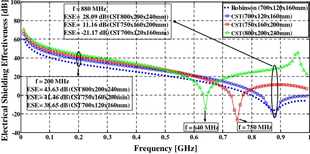
Figure 4. Simulation results of ESE versus frequency for case 1, 2 and 3 on Table 1.
aperture width and pthe probe position. For all cases, the frequency range is 0–1 GHz. The thickness
of metallic enclosure is 2 mm; the incident angle is zero (θ= 0◦) due to the normal incident plane wave; the angle of polarization is 90◦ (α = 0◦). The effect of enclosure size, aperture size, probe location, aperture shape, multiple apertures and aperture configuration are investigated as indicated in Figs. 4– 14. Generally, for 0–1 GHz interval, ESE decreases with increased frequency until resonant frequencies. Onwards resonant frequencies, ESE increases with increased frequency. This result can be explained as that wave length is inversely correlated with frequency. If the wave length is low (with increased frequency), higher amplitude of electrical field get in to aperture of enclosure. At resonance frequency, ESE is negative, which means that there are such sources which lead to the rise of noise and interference. That is the unwanted case for shielding and why we have high ESE at low frequencies in CST model.
3.1. Effect of Enclosure Size
In Fig. 4 for cases 1, 2 and 3, ESE is 43.63, 41.46 and 38.65 dB at 200 MHz (below resonant frequency)
and 28.09, 11.16 and −16.12 dB, respectively at 880 MHz (above resonant frequency). So, when the
enclosure size is increased from 700×120×160 mm to 800×200×240 mm, ESE is 4.98 dB higher at
200 MHz and 44.2 dB higher at 880 MHz. At same frequencies, ESE gets higher with increased enclosure size. These results can be explained with Eqs. (2a), (2b), (2c) and (2d) as given below [22]. In these
equations for TE (Transverse Electric) modes, the amplitude of electric fieldEx andEy which gets into
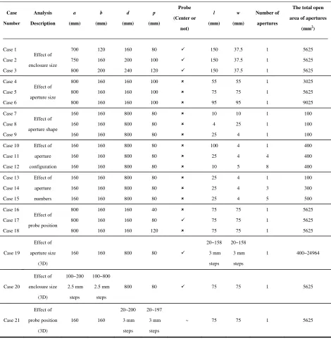
Table 1. The cases and its parameter values used in CST simulation to calculate ESE. Case Number Analysis Description a (mm) b (mm) d (mm) p (mm) Probe (Center or not) l (mm) w (mm) Number of apertures
The total open
area of apertures
(mm2)
Case 1
Effect of
enclosure size
700 120 160 80 150 37.5 1 5625
Case 2 750 160 200 100 150 37.5 1 5625
Case 3 800 200 240 120 150 37.5 1 5625
Case 4
Effect of
aperture size
800 160 160 100 55 55 1 3025
Case 5 800 160 160 100 75 75 1 5625
Case 6 800 160 160 100 95 95 1 9025
Case 7
Effect of
aperture shape
160 160 800 80 10 10 1 100
Case 8 160 160 800 80 4 25 1 100
Case 9 160 160 800 80 25 4 1 100
Case 10 Effect of
aperture
configuration
160 160 800 80 100 4 1 400
Case 11 160 160 800 80 25 4 4 400
Case 12 160 160 800 80 10 5 8 400
Case 13 Effect of
aperture
numbers
160 160 800 80 25 4 1 100
Case 14 160 160 800 80 25 4 3 300
Case 15 160 160 800 80 25 4 5 500
Case 16
Effect of
probe position
800 160 160 40 75 75 1 5625
Case 17 800 160 160 80 75 75 1 5625
Case 18 800 160 160 120 75 75 1 5625
Case 19
Effect of
aperture size
(3D)
160 160 800 80
20~158 3 mm steps 20~158 3 mm steps 1 400~24964 Case 20 Effect of enclosure size (3D) 100~200 2.5 mm steps 100~800 2.5 mm steps
800 80 75 75 1 5625
Case 21 Effect of probe position (3D) 160 160 20~200 3 mm steps 20~197 3 mm steps
~ 75 75 1 5625
ESE in CST model via increasing enclosure size.
Ex = βy
ε Amnpcos (βxx) sin (βyy) sin (βzz) (V/m) (2a)
Ey = −βx
ε Amnpsin (βxx) sin (βyy) sin (βzz) (V/m) (2b)
Ez = 0 (V/m) (2c)
Here βx, βy, and βz are the components of phase constants of TE mode plane EM wave; Amnp is the amplitude of the electric field;ε is the dielectric constant of the medium where m,n,p= 0,1,2,3, . . .,
exceptm=n= 0.
As seen in Fig. 4, for cases 1, 2 and 3, resonance frequency is 640, 750 and 880 MHz, respectively, which means that resonance frequency decreases with increased enclosure size. This result can be explained with Eq. (3) [22], and resonance frequency decreases with increased enclosure size values (a,
band d). That is why in case 3, lower resonance frequency is 640 MHz. The resonance frequency of TE
mode is given by
(fresonance)T Emnp = 1 2π√με
mπ
a
2
+
nπ
b
2
+
pπ
d
2
(Hz) (3)
where m, n, p = 0,1,2,3, . . ., except that m = n = 0 and that μ and ε are the permeability and dielectric constant of the enclosure material, respectively.
3.2. Effect of Aperture Size
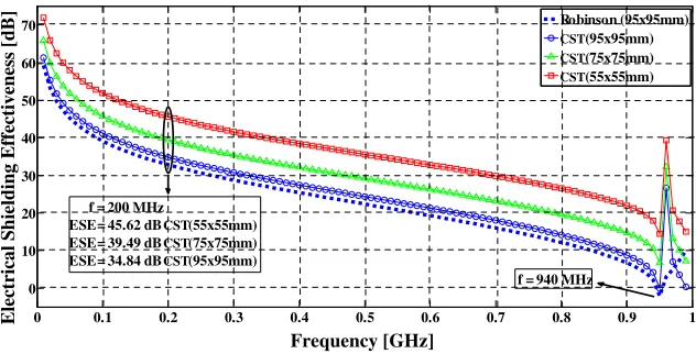
For cases 4, 5 and 6, ESE is 45.23, 39.49 and 34.84 dB, respectively at 200 MHz, which means that ESE
gets 10.78 dB higher when the aperture size is decreased from 95×95 mm to 55×55 mm. At the same
frequencies, ESE has increased with decreased aperture size. This situation can be explained with Eq. (4) [22] as:
Pe= 12
SRe
E×H∗
·dS(W) (4)
Pe is the existing total power of surfaceS. Increased aperture size means that area of aperture increases by differential surface elementsdS as seen in Eq. (4). So, ESE gets higher with increased aperture size. As seen in Fig. 5, for cases 4, 5 and 6, ESE has the same resonance frequency 940 MHz in these cases due to the same enclosure size as discussed before with Eq. (3).
0 0.1 0.2 0.3 0.4 0.5 0.6 0.7 0.8 0.9 1
0 10 20 30 40 50 60 70
Electrical Shielding Effectiveness [dB]
Robinson (95x95mm)
CST (95x95mm)
CST (75x75mm)
CST (55x55mm)
f = 940 MHz f = 200 MHz
ESE = 45.62 dB CST (55x55mm) ESE = 39.49 dB CST(75x75mm) ESE = 34.84 dB CST (95x95mm)
Frequency [GHz]
Figure 5. Simulation results of ESE versus frequency for case 4, 5 and 6 on Table 1.
3.3. Effect of Aperture Shape
For cases 7, 8 and 9, the total open area of apertures is fixed as 100 mm2. Resonance frequency has no
change as 955 MHz, as explained with Eq. (3). ESE changes with the ratio of aperture length/width. For cases 7, 8 and 9, the ratios of aperture length/width are 1, 0.16 and 6.25 as seen in Fig. 6. When the aperture has long length with short width, ESE gets higher. At the same frequency sample point at
200 MHz, ESE is 86.13, 71.98 and 99.86, respectively. When the aperture size is modified from 4×25 mm
to 25×4 mm, ESE gets 27.88 dB higher. This result can be explained with Fig. 7. Perpendicular
field and the location of aperture width have the same direction, which means that when the aperture width is higher, high amplitude of electric field gets into aperture of enclosure. Then, from Eqs. (2a)
and (2b), ESE becomes worse with increased amplitudeAmnp of electric field. Finally, ESE is decreased
with increased aperture width. It can be remembered that cases 7, 8 and 9’s aperture widths are 10, 25 and 4 mm, respectively. ESE has the best value 99.86 dB when aperture width is at the lowest value of 4 mm @ 500 MHz. As a result, ESE changes with polarization of plane wave and the direction of electric field according to the aperture shape (in this situation, it is aperture width).
0 0.1 0.2 0.3 0.4 0.5 0.6 0.7 0.8 0.9 1
0 20 40 60 80 100 120
Frequency [GHz]
Electrical Shielding Effectiveness [dB]
Robinson (4x25mm)
CST(4x25mm)
CST (10x10mm)
CST (25x4mm) The total open areas are fixed as 100mm2 and number of aperture is one in this case
f = 955 MHz f = 200 MHz
ESE = 99.86 dB CST (25x4mm) ESE = 86.13 dB CST (10x10mm) ESE = 71.98 dB CST (4x25mm)
Figure 6. Simulation results of ESE versus frequency for case 7, 8 and 9 on Table 1.
Er kˆ
Hr
Figure 7. The location of plane wave and its parameters: Perpendicular polarization of TE mode means the angle of polarization (α= 90◦) (the angle between electric field and travelling wave direction
z-axis), the incident angle θ = 0◦ (the angle between traveling wave ˆk and z-axis) and other incident angle (Φ = 90◦) (the angle from positivex-axis onx-y plane up to 360◦).
3.4. Effect of Aperture Configuration
For cases 10, 11 and 12, resonance frequency does not change at 935 MHz as indicated from Eq. (3) and as seen in Fig. 8. As discussed before for perpendicular polarization, aperture width of enclosure and total open area of aperture of enclosure affect ESE. For cases 10, 11 and 12, aperture width is nearly
the same as 4 and 5 mm. The total open area of aperture(s) is fixed as 400 mm2. In this situation,
0 0.1 0.2 0.3 0.4 0.5 0.6 0.7 0.8 0.9 1 0
20 40 60 80 100 120
Frequency [GHz]
Electrical Shielding Effectiveness [dB]
Robinson n=8 (8 apertures with 10x5mm) CST n=8 (8 apertures with 10x5mm)
CST n=4 (4 apertures with 25x4mm) CST n=1 (1 apertures with 100x4mm)
f = 935 MHz The total open area is fixed as 400mm2
f = 200 MHz
ESE = 90.42 dB CST n=1 (1 apertures with 100x4mm) ESE = 81.85 dB CST n=4 (4 apertures with 25x4mm) ESE = 64.12 dB CST n=8 (8 apertures with 10x5mm)
Figure 8. Simulation results of ESE versus frequency for case 10, 11 and 12 on Table 1.
3.5. Effect of Number of Apertures
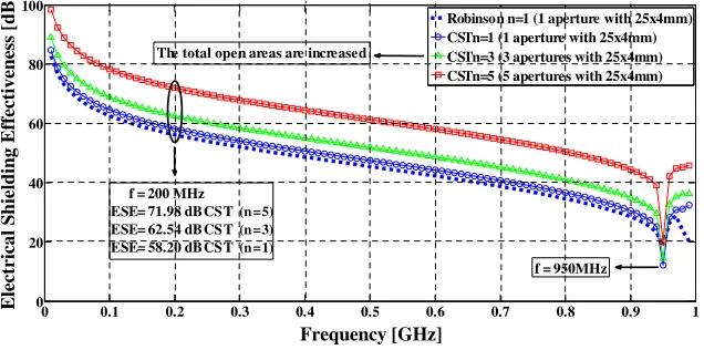
For cases 13, 14 and 15, resonance frequency has no change as 950 MHz, as discussed in Section 3.4. It is better to minimize number of apertures on enclosure when the total open area of aperture(s) is fixed. While the total open area aperture(s) is increased for cases 13, 14 and 15, number of aperture(s) is analyzed here. At the same frequency, ESE gets higher with decreased number of apertures. In Fig. 9 for cases 13, 14 and 15, ESE is 71.98, 62.54 and 71.98 dB, respectively, at 200 MHz. When the number of apertures is increased from 1 to 5, ESE gets 13.78 dB higher. ” The reason of this improvement (total open area of aperture) is explained in Section 3.2 that ESE gets higher with increased aperture size. While the number of apertures decreases from 8 to 1, as noted before in Section 3.4, ESE gets 26.3 dB higher. So, simulations tell us that the effect of aperture number is more effective than total area of apertures on electric shielding.
0 0.1 0.2 0.3 0.4 0.5 0.6 0.7 0.8 0.9 1
0 20 40 60 80 100
Frequency [GHz]
Electrical Shielding Effectiveness [dB]
Robinson n=1 (1 aperture with 25x4mm) CST n=1 (1 aperture with 25x4mm) CST n=3 (3 apertures with 25x4mm) CST n=5 (5 apertures with 25x4mm)
f = 950 MHz The total open areas are increased
f = 200 MHz ESE = 71.98 dB CST (n =5) ESE = 62.54 dB CST (n=3) ESE= 58.20 dB CST (n=1)
Figure 9. Simulation results of ESE versus frequency for case 13, 14 and 15 on Table 1.
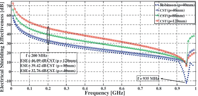
3.6. Effect of Probe Position
For cases 16, 17 and 18, resonance frequency has no change as 935 MHz. At the same frequency, when the distance between probe location and aperture is far, ESE gets better. In Fig. 10, for cases 16, 17 and
18, ESE is 32.76, 39.42 and 46.09 dB, respectively at 200 MHz. When the probe position pof enclosure
0 0.1 0.2 0.3 0.4 0.5 0.6 0.7 0.8 0.9 1 -10
0 10 20 30 40 50 60 70
Frequency [GHz]
Electrical Shielding Effectiveness [dB]
Robinson (p=40mm)
CST (p=40mm)
CST (p=80mm)
CST (p=120mm)
f = 935 MHz f = 200 MHz
ESE = 46.09 dB CST (p = 120mm) ESE = 39.42 dB CST (p = 80mm) ESE = 32.76 dB CST (p = 40mm)
Figure 10. Simulation results of ESE versus frequency for case 16, 17 and 18 on Table 1.
input power of the transmitting antenna Pt. The term (λ/4πR)2 is called free-space loss factor, and
it takes into account the losses due to the spherical spreading of the energy by the antenna. G0t and
G0r are the gains of transmitting and receiving antennas in the directions 0tand 0r, respectively [23].
In simulations, plane wave is out of enclosure (Transmitter propagates plane wave), and receiver probe is in the enclosure. Eq. (5) tells us that receiver power is inversely proportional to squared distance. While the transmitter wave is travelling, in simulation model, onz-axis as seen in Fig. 7, power of wave decreases. When the probe distance is increased, power of wave decreases. Friis transmission equation is given as:
Pr Pt =
λ
4πR
2
G0tG0r (5)
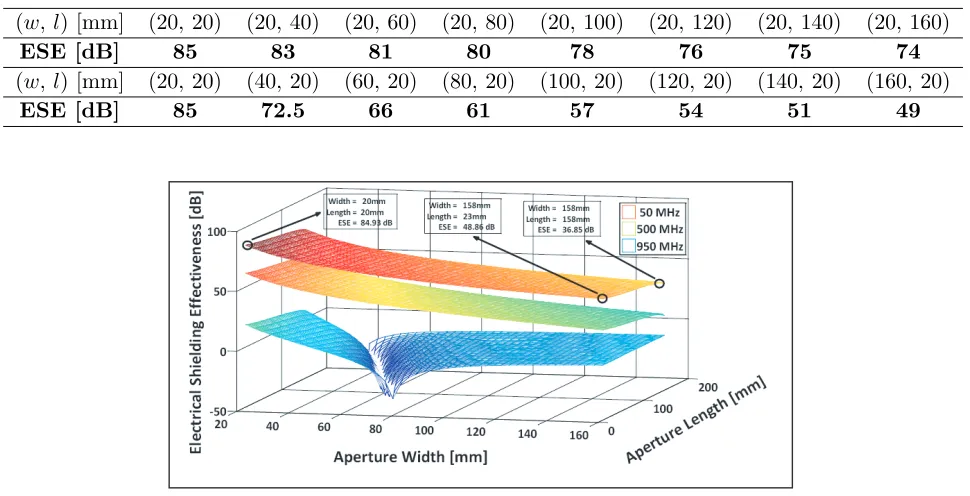
3.7. Effect of Aperture Sizes by 3D Investigation
For cases 4, 5 and 6, three apertures which have different sizes are investigated as discussed before in Fig. 5. For case 19 in Fig. 11, aperture width and length are changed linearly from 20 to 158 mm with 3 mm increment. 47 apertures having different lengths, 47 apertures having different widths, totally 2209
(47×47) different aperture sizes are used. So, all possible square and rectangular sizes are computed
for ESE. From the top to bottom, the selected frequencies are 50, 500 and 950 MHz, respectively. ESE gets better with decreased frequency as discussed before. Since 950 MHz is resonance frequency or too close to resonance frequency, there is a valley at this frequency.
At 50 MHz, when the aperture length is fixed as 20∼23 mm and the aperture width increased from
20 to 158 mm, ESE gets 36.08 dB lower as seen in Fig. 11. This decrease is due to increased total open area of apertures on enclosure as discussed before in Section 3.2. When the aperture length is fixed and the width increased at the same time, the total open area of aperture is increased, so the influence of power keeps ESE lower. At 50 MHz, when the aperture width is fixed as 158 mm and the aperture length increased from 23 to 158 mm, ESE gets 12.01 dB lower. This decrease can also be explained in Section 3.2.
Figure 11. Simulation results of ESE versus aperture width and length for case 19 (Perpendicular Polarization).
Table 2. ESE values versus aperture width and length (Aperture width and length size modified 20 mm each).
(w,l) [mm] (20, 20) (20, 40) (20, 60) (20, 80) (20, 100) (20, 120) (20, 140) (20, 160)
ESE [dB] 85 83 81 80 78 76 75 74
(w,l) [mm] (20, 20) (40, 20) (60, 20) (80, 20) (100, 20) (120, 20) (140, 20) (160, 20)
ESE [dB] 85 72.5 66 61 57 54 51 49
Figure 12. Simulation results of ESE versus aperture width and length for case 19 (Parallel Polarization).
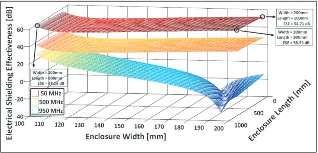
3.8. Effect of Enclosure Size by 3D Investigation
As discussed before in Fig. 4, for cases 1, 2 and 3, three enclosures which have different sizes are designed. In Fig. 13 for case 20, enclosure depth is fixed as 160 mm for all situations. Enclosure length (a) is varied
linearly from 100 to 800 mm with 18 mm increment. Enclosure width (b) is varied linearly from 100 to
200 mm with 2.55 mm increment. 41 enclosures having different lengths, 280 enclosures having different
widths, totally 11521 (41×281) different enclosure sizes have been used. So, all possible enclosure
Figure 13. Simulation results of ESE versus enclosure width and length for case 20 on Table 1.
before. Since 950 MHz is resonance frequency or too close to resonance frequency, there is a valley at 950 MHz.
At 50 MHz, when the enclosure length (a) is fixed as 800 mm and the enclosure width (b) varied
from 100 to 200 mm, ESE gets just 0.41 dB better. However, when the enclosure width (b) is fixed as
200 mm and enclosure length (a) modified from 100 to 800 mm, ESE gets just 3.88 dB better. The effect
of modified values of sizes (100 mm for enclosure width and 700 mm for enclosure length) on ESE is only 0.41 dB and 3.88 dB, so these results can be ignored. The same conclusions can be seen also at 500 MHz. But similar conclusion is not seen at resonance frequency or the frequency close to resonance frequency. For example, at 950 MHz when enclosure width is decreased from 200 to 100 mm, ESE is significantly
increased from −17 to 26 dB. It means that there is a 43 dB improvement on ESE. At 950 MHz when
enclosure length is decreased from 800 to 100 mm, ESE is increased from−16 to−11 dB. It means that
there is only 5 dB improvement on ESE in this situation. At 50 and 500 MHz, there is no significant effect. At 950 MHz, the effect of enclosure width (43 dB) is more important than the effect of enclosure width (5 dB) due to the direction of incidence electric field as discussed before. That is why in resonance region, designers need optimization to rescue devices from negative shielding.
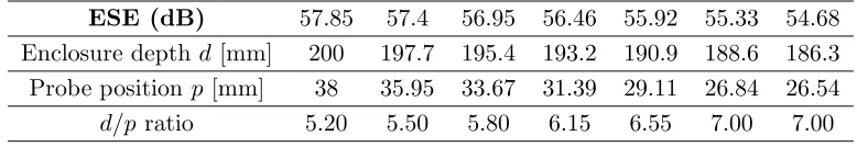
3.9. Effect of Probe Position and Enclosure Depth by 3D Investigation
As discussed before in Fig. 10, effect of three different probe positions on ESE is investigated. In Fig. 14
for case 21, the probe position (p) and enclosure depth (d) are varied from 20 to 200 mm with 2.3 mm
increment. 61 enclosures having different depths, 60 enclosures having different probe positions, totally
3660 (61×60) different enclosure cases have been used. All situations in which enclosure depth (d) is
bigger than the probe position (p) have been analyzed.
At 50 MHz, while the enclosure depth (d) is fixed as 200 mm and the probe position (p) moved
away from 20 to 197 mm, ESE gets 58.7 dB better. The reason for these results is the same as that in
Section 3.6. At 500 MHz, when the probe position (p) is fixed as 60 mm and the enclosure depth (d)
moved away from 63.29 to 200 mm, ESE gets 36 dB better (from 43.85 to nearly 80 dB).
Except resonance frequencies (at 50 and 500 MHz), we recommend that it is better to increase
enclosure depth (d) and probe position (p). But at resonance frequencies (at 950 MHz here), when the
enclosure depth is high and probe position low, there is a different and important region as seen in the left of Fig. 14. There is an improvement on ESE in this special region as also seen in Table 3.
The highest ESE values at 950 MHz are seen in Table 3 for different 7 points where the ratio of d/pis
Figure 14. Simulation results of ESE versus probe position and enclosure depth for case 21 on Table 1.
Table 3. Investigation of enclosure depth (d), probe position (p) and the ratio of d/p at 950 MHz on Figure 14.
ESE (dB) 57.85 57.4 56.95 56.46 55.92 55.33 54.68
Enclosure depthd[mm] 200 197.7 195.4 193.2 190.9 188.6 186.3
Probe positionp [mm] 38 35.95 33.67 31.39 29.11 26.84 26.54
d/p ratio 5.20 5.50 5.80 6.15 6.55 7.00 7.00
4. CONCLUSION AND FUTURE WORK
Metallic shielding enclosures are used to reduce radiation from external electromagnetic fields and exudation effects from interior devices as examples which are mainboard circuits, Wi-Fi transceivers, RAMs, sub-boards, solid-state drives (SSD), etc. in a computer case, laptop or TV. As a fact, the required slots and apertures on enclosures for heat allocation, ventilation, I/O cable, etc. induce the coupling route of EMI from the inside to outside. So, the investigation of SE becomes important for designing metallic enclosures of EMI sensitive devices in manufacturing process. When ESE is negative, it is a harmful situation for devices as known. Thus, the device producers need to calculate resonance frequency of enclosure at first against electric interference before the design of device enclosure. ESE is always higher in lower frequencies, so devices should be operated in small frequency whenever possible to get higher performance and quality. We give detailed comments depending on simulated results of ESE parameters noted in Section 3 as the following:
√
First, increasing the enclosure size makes ESE higher, and that is why designers should prefer larger size of enclosure. Second, since the operating frequency of device and the resonance frequency of enclosure are the same or close to each other, a) producers need to adjust device parameters to change operating frequency, and b) they need to modify enclosure size (prefer increasing as discussed above) to change resonance frequency.
√
When aperture shape is square, using small aperture size on enclosures makes ESE better. In this situation, designers are required to identify the polarization of incident electric field. For parallel polarization decreasing aperture length and for perpendicular polarization decreasing aperture width are more effective on ESE. First, designers should decrease aperture width for perpendicular
polarization. Second, if the polarization is fixed, they need locate the aperture on enclosure
√
Minimizing number of apertures makes ESE better while total open area of aperture(s) is fixed. So, device producers should use fewer apertures. But when the total area of aperture(s) is not fixed, increasing number of used apertures makes ESE higher, so designers should use more apertures in this manner.
√
Increasing probe distance gets ESE higher. So, it is better for designers to locate device/circuit as far away from aperture(s) of enclosure as possible and to find the best direction of device according to the aperture size and polarization to improve quality. But at resonance frequencies, there is a
special region whered/pratio is 5.2–7 and ESE the highest, and optimization engineers should not
ignore this effective region for resonance frequencies.
In computer enclosures there are many apertures with different geometrical shapes for airing, I/0 connections and other purposes. This paper provides that insight about effect of rectangular aperture number, configuration, etc. on ESE. In our future work, for a sample computer box, the effect of round, hexagonal and triangle apertures on ESE will be investigated. Then, according to these effects, location and polarization of mainboard, hard disc, airing fan, etc. will be tried to determine.
ACKNOWLEDGMENT
This work was supported by the Department of Scientific Research Projects in S¨uleyman Demirel
University named as “Investigation the effect on total electromagnetic emission distribution of metallic enclosure topology” and in Turkish “Metalik kutulama topolojisinin toplam elektromanyetik emisyon
da˘gılımına etkisinin incelenmesi” [Project Number: 4384-D2-15].
REFERENCES
1. Ansari, M. S., S. V. G. Ravindranath, M. S. Bhatia, B. Singh, and C. P. Navathe, “Electromagnetic coupling through apertures and shielding effectiveness of a metallic enclosure housing electro-optic
pockels cell in a high power laser system,”International Journal of Applied Electromagnetics and
Mechanics, Vol. 42, No. 2, 191–199, 2013.
2. IEEE, “Standard method for measuring the effectiveness of electromagnetic shielding enclosures,” IEEE Std 299TM-2006 (R2012), 2012.
3. Robinson M. P., T. M. Benson, C. Christopoulos, J. F. Dawson, M. Ganley, A. Marvin, S. Porter, and D. W. Thomas, “Analytical formulation for the shielding effectiveness of enclosures with
apertures,”IEEE Transactions on Electromagnetic Compatibility, Vol. 40, No. 3, 240–248, 1998.
4. Solin J. R., “Formula for the field excited in a rectangular cavity with an aperture and lossy walls,” IEEE Transactions on Electromagnetic Compatibility, Vol. 57, No. 2, 203–209, 2015.
5. Nobakhti M., P. Dehkhoda, and A. Tavakoli, “Improved modal method of moments technique
to compensate the effect of wall dimension in shielding effectiveness evaluation,” IET Science,
Measurement & Technology, Vol. 8, No. 1, 17–22, 2014.
6. Liu E., P.-A. Du, and B. Nie, “An extended analytical formulation for fast prediction of shielding
effectiveness of an enclosure at different observation points with an off-axis aperture,” IEEE
Transactions on Electromagnetic Compatibility, Vol. 56, No. 3, 589–598, 2014.
7. Hao, C. and D. Li, “Simplified model of shielding effectiveness of a cavity with apertures on different
sides,”IEEE Transactions on Electromagnetic Compatibility, Vol. 56, No. 2, 335–342, 2014.
8. Belkacem, F. T., M. Bensetti, A.-G. Boutar, D. Moussaoui, M. Djennah, and B. Mazari, “Combined
model for shielding effectiveness estimation of a metallic enclosure with apertures,”IET Science,
Measurement & Technology, Vol. 5, No. 3, 88–95, 2011.
9. Nie, B.-L. and P.-A. Du, “An efficient and reliable circuit model for the shielding effectiveness
prediction of an enclosure with an aperture,”IEEE Transactions on Electromagnetic Compatibility,
Vol. 57, No. 3, 357–364, 2015.
10. Wang, C.-C., C.-Q. Zhu, X. Zhou, and Z.-F. Gu, “Calculation and analysis of shielding effectiveness
of the rectangular enclosure with apertures,” Applied Computational Electromagnetics Society
11. Karami, H., R. Moini, S. H. Sadeghi, H. Maftooli, M. Mattes, and J. R. Mosig, “Efficient analysis of shielding effectiveness of metallic rectangular enclosures using unconditionally stable time-domain
integral equations,” IEEE Transactions on Electromagnetic Compatibility, Vol. 56, No. 6, 1412–
1419, 2014.
12. Hussein, K. F., “Spatial filter housing for enhancement of the shielding effectiveness of perforated
enclosures with lossy internal coating: Broadband characterization,” International Journal of
Antennas and Propagation, Vol. 2, No. 8, 2013.
13. Xiong, R., B. Chen, Z. Y. Cai, and Q. Chen, “A numerically efficient method for the FDTD analysis of the shielding effectiveness of large shielding enclosures with thin-slots,”International Journal of Applied Electromagnetics and Mechanics, Vol. 40, No. 4, 251–258, 2012.
14. Azizi, H., F. TaharBelkacem, D. Moussaoui, H. Moulai, A. Bendaoud, and M. Bensetti, “Electromagnetic interference from shielding effectiveness of a rectangular enclosure with apertures–
circuital approach, FDTD and FIT modeling,”Journal of Electromagnetic Waves and Applications,
Vol. 28, No. 4, 494–514, 2014.
15. Lei, J.-Z., C.-H. Liang, and Y. Zhang, “On shielding effectiveness of metallic cavities with apertures
by combining parallel FDTD method with windowing technique,” Progress In Electromagnetics
Research, Vol. 74, 85–112, 2007.
16. Dehkhoda, P., A. Tavakoli, and R. Moini, “Fast calculation of the shielding effectiveness for a
rectangular enclosure of finite wall thickness and with numerous small apertures,” Progress In
Electromagnetics Research, Vol. 86, 341–355, 2008.
17. Dehkhoda, P., A. Tavakoli, and M. Azadifar, “Shielding effectiveness of an enclosure with finite wall thickness and perforated opposing walls at oblique incidence and arbitrary polarization by
GMMoM,” IEEE Transactions on Electromagnetic Compatibility, Vol. 54, No. 4, 792–805, 2012.
18. Basyigit, I. B., M. F. Caglar, and S. Helhel, “Magnetic shielding effectiveness and simulation
analysis of metalic enclosures with apertures,” Proceedings of the 9th International Conference on
Electrical and Electronics Engineering (ELECO), 328–331, Bursa, Turkey, November 2015.
19. Basyigit, I. B., P. D. Tosun, S. Ozen, and S. Helhel, “An affect of the aperture length to
aperture width ratio on broadband shielding effectiveness,”Proceedings of the XXXth URSI General
Assembly and Scientific Symposium, 1–4, Istanbul, Turkey, August–November 2011. 20. C. S. Technology, CST-EMC Studio, 2015, Available: www.cst.com.
21. Celozzi, S. and R. Araneo, “Alternative definitions for the time-domain shielding effectiveness of
enclosures,”IEEE Transactions on Electromagnetic Compatibility, Vol. 56, No. 2, 482–485, 2014.
22. Balanis, C. A.,Advanced Engineering Electromagnetics, Wiley, New York, 2012.