Copyright1998 by the Genetics Society of America
Combining Different Line Crosses for Mapping Quantitative Trait Loci
Using the Identical by Descent-Based Variance Component Method
Chongqing Xie, Damian D. G. Gessler and Shizhong Xu
Department of Botany and Plant Sciences, University of California, Riverside, California 92521 Manuscript received October 1, 1997
Accepted for publication February 20, 1998
ABSTRACT
Mapping quantitative trait loci (QTLs) is usually conducted with a single line cross. The power of such QTL mapping depends highly on the two parental lines. If the two lines are fixed for the same allele at a putative QTL, the QTL is undetectable. On the other hand, if a QTL is segregating in the line cross and is detected, the estimated variance of the QTL cannot be extrapolated beyond the statistical inference space of the two parental lines. To reduce the likelihood of missing a QTL and to increase the statistical inference space of the estimated QTL variance, we present a consensus QTL mapping strategy. We adopt the identical by descent (IBD)-based variance component method originally applied to human linkage analysis by combining multiple line crosses as independent families. We explore the properties of consensus QTL mapping and demonstrate the method with F2, backcross (BC), and full-sib (FS) families. In addition, we examine the effects of the QTL heritability, marker informativeness, QTL position, the number of families, and family size. We show that F2families notably outperform BC and FS families in detecting a QTL. There is a substantial reduction in the standard deviation of the estimated QTL position and the separation of the QTL and polygenic variance. Finally, we show that the power to detect a QTL is greater when using a small number of large families than a large number of small families.
L
INE crossing is a common experimental design for individuals within that line cross; i.e., the QTL variance is formulated as conditional on the cross. As a result, mapping quantitative trait loci (QTLs) in plantsthe variance itself is a variable that differs from one and laboratory animals. Crosses are initiated from at
cross to another. Therefore, a QTL variance estimated least two inbred lines, such as backcrosses (BC), F2, and
from a single line cross cannot be extended to a statisti-more derived generations. Statistical methods are well
cal inference space beyond that cross. In addition, the developed for QTL mapping using such line crossing
number of founder alleles at any locus is expected to data (LanderandBotstein 1989;Haley andKnott
be small in a line cross. For instance, there are at most 1992;Martı´nezandCurnow1992;Jansen1993;Zeng
two alleles at each locus in an F2 family. With such a
1994). These methods are mainly designed to handle
single line cross, one’s entire effort is invested in this a single line cross. The characteristics of line crossing
single large family. If the two founder alleles of a QTL experiments are: (1) a small number of parental lines
are polymorphic, then detection of the QTL is possible are involved, (2) the linkage phases of the parental
with a relatively large family. On the other hand, if the markers are known, and (3) family sizes are usually
two parental lines are fixed for the same allele at a large. These properties allow the effects of a gene
substi-particular QTL, then this QTL is undetectable, indepen-tution to be tested directly. The methods developed by
dent of the sample size. To increase the statistical infer-the above authors all test infer-the effects of a gene
substitu-ence space of the estimated QTL variance and ensure tion (the first moments) and therefore are referred to
that polymorphic alleles are present in the parental as the fixed model approach (XuandAtchley1995).
gene pool, one needs to sample a sufficient number Quantitative geneticists are interested not only in
de-of parents (Muranty1996). This can be achieved by tecting QTLs and locating their positions, but also in
combining data from multiple line crosses. estimating the contribution of the detected QTLs to
Suppose that there are 10 F2families derived from 10
a trait. The contribution of a QTL, however, is only
pairs of inbred lines. What is the appropriate statistical meaningful when expressed relative to the total
pheno-method for analyzing the data from these F2families?
typic variance. Therefore, the effect of a QTL is actually
One may simply extend the regression approach to fit measured by its variance. In a single line cross, the
2 additional parameters, 1 mean and 1 gene substitution QTL variance is relative to the genetic variance among
effect, for each F2 family added to the data set. This
means estimating 20 parameters and testing 10 additive effects. If dominance deviations are considered, 10
addi-Corresponding author: Shizhong Xu, Department of Botany and Plant
tional terms must be estimated and tested. In a single-Sciences, University of California, Riverside, CA 92521-0124.
E-mail: [email protected] line, fixed model, one can easily convert the effect of
1140 C. Xie, D. D. G. Gessler and S. Xu
being twice the coancestry coefficients for the polygenic
com-a gene substitution into the vcom-aricom-ance vicom-a s2
g 5 a2/2,
ponent, and I is the identity matrix.
where a is the average effect of a gene substitution
Under the assumption that y is multivariate normal andP
(Falconer andMackay1996). But as the number of
is known, the likelihood function for a particular family is
parameters increases, extension of this method becomes
complicated. L(buyP)5 1
(2p)n/2uVu1/2exp[2
1⁄2(y21m)TV21(y21m)],
Data from multiple line crosses, such as diallelic and
four-way crosses, can occasionally be analyzed using the whereb 5[m s2
gs2as2e]Tare the unknown parameters and the superscript T stands for matrix transposition.
methods ofRebaiandGoffinet(1993) andXu(1996a).
Assume that families are independent so that the overall
A survey of the literature shows that the most popular
likelihood function for multiple families is simply the product
computer software, such as MAPMAKER/QTL (
Lin-of these family-specific likelihoods. Therefore, the overall log coln et al. 1993), QTL Cartographer (Basten et al.
likelihood for N families is:
1997), MapQTL (van OoijenandMaliepaard1996),
and MQTL (TinkerandMather1995), are designed L5
o
N
k51
log[Lk(buykPk)],
to handle only a single line cross.
where Lk(buykPk) represents the likelihood of the kth family.
In contrast to the difficulties of the fixed model, the
To test the presence of a QTL, a log likelihood ratio test
IBD-based variance component method initially
devel-statistic is used, which isL 5 22(L02L1), where L1is the
oped for human genetic studies can handle multiple log likelihood value evaluated at the maximum likelihood families (Haseman and Elston 1972). This method solution under the alternative model (b15[m s2
g s2as2e]T) and
has been referred to as the random model approach L0is the log likelihood value evaluated at the maximum likeli-hood solution under the null model (b05[m s2
as2e]T).
because the QTL variance is directly estimated and
The IBD value between two sibs at a QTL: Because of
tested (XuandAtchley1995). To separate the QTL
inbreeding, the IBD values among F2individuals are different
variance from the polygenic variance, the IBD-based
from those among regular full sibs. If the parental lines are
approach relies on variation in the proportion of genes fixed for alternative QTLs, then F2individuals have three possi-IBD shared by relatives at the putative QTL. The random ble genotypes at a QTL: QQ, Qq, and qq. Given the genotypic configuration of individuals i and j, the IBD value is measured
model approach is adopted here for combining data
as
from different line crosses because each line cross is effectively a different family.
Before one can apply the random model approach to p
ij52uij5
5
2 for QQ-QQ or qq-qq 1 for QQ-Qq, qq-Qq, or Qq-Qq 0 for QQ-qq,
,
line crosses, one needs to adjust for the fact that regular full-sib (FS) families and families of line crosses differ
wherepijare the ijth elements ofPanduijisMale´cot’s (1948)
in that the latter involves inbreeding (for example, an
coefficient of coancestry. Note that while pij between
non-F2 individual is equivalent to a progeny resulting from inbred, full sibs ranges from zero to one, under inbreeding
a selfing parent). The traditional IBD-based method pijranges from zero to two. In this usage,pijis not interpreted
as the proportion of alleles IBD, but rather as twice the
coeffi-must therefore be modified to reflect the inbreeding
cient of coancestry (Kempthorne1955;Harris1964; Cock-effect. Our purpose here is to develop such an
IBD-erham1983). For example, when the two individuals have a based random model methodology for combining data genotypic configuration of QQ-Qq, the coefficient of coances-from different line crosses. We examine two types of try is
line crosses: F2and BC. We then compare the results
uij51⁄4[Pr(Q;Q)1Pr(Q;q)1Pr(Q;Q)1Pr(Q;q)]
with regular noninbred, FS families.
51⁄4[1101110]51⁄2.
Without inbreeding, the IBD value of an individual with
STATISTICAL METHODS itself (p
jj) always takes a value of 1. Under inbreeding,pjjcan be greater than 1, depending on whether the individual is
Linear model and likelihood function: We combine line
homozygous or heterozygous, i.e., crosses by treating each line cross as a family and using a
multipoint QTL mapping methodology. Consider a family
pjj511φj5
5
2 if QQ-QQ or qq-qq
1 if Qq-Qq ,
with n individuals; the phenotypic value (yi) of the ith individ-ual is described as yi5 m 1gi1ai1ei(Goldgar1990;Xu
andAtchley 1995), where mis the overall mean, g
iis the where φj is the inbreeding coefficient of individual j at the additive effect of a putative QTL with mean 0 and variance QTL. Here,pjjcan be interpreted as 1 plus the inbreeding s2
g, aiis the polygenic effect (excluding gi) with mean 0 and coefficient (Harris1964;Cockerham1983).
variance s2
a, and ei is the residual error distributed as The elements in the additive relationship matrix A are IBD
N(0,s2
e). Inclusion of a dominance effect is discussed later. values of the polygenic component and can be obtained by In matrix notation, the model is y51m 1g1a 1e. The taking the unconditional expectation ofpij. In an F2family, expectation and variance of the model are E(y) 51m and Ahas elements of Aij5E(pij)51 and Ajj5 E(pjj)5 3⁄2, in Var (y)5 V 5Ps2
g 1 As2a 1 Ise2, respectively, where 1 is a contrast to Aij51⁄2and Ajj51 in a regular FS family. column vector of order n,P5 {pij}n3nis a square matrix of In BC populations, thep’s are derived similarly. They are order n with the element of the ith row and the jth column
being the shared IBD value between sibs i and j at the QTL, p
ij52uij5
5
2 for QQ-QQ
1 for QQ-Qq or Qq-Qq
for between individuals and nent to the total phenotypic variance was 50%, with 25% for each component. We referred to this as the standard setting. To examine the effect of different factors on the perfor-pjj511φj5
5
2 for QQ-QQ
1 for Qq-Qq mance of the methods, we varied each of the following factors successively: (a) the number of families3 family size: 203 for the individual with itself. A has elements of Aij55⁄4and 25, 25032, or 50032, (b) QTL heritability, h2g50.10 (s2a5
Ajj53⁄2. 12.5,s2g 55.0, ands2e 532.5) or h2g 50.5 (s2a512.5,s2g 5
Inferring the IBD value of a QTL from markers:The IBD 25.0, ands2
e5 12.5), (c) true QTL position at 10 cM or 30 value is completely determined by the genotypes of two indi- cM, (d) low marker information (two alleles, one with a fre-viduals at the QTL of interest. The actual genotype of an quency of 0.9 and the other with 0.1) and high marker infor-individual, however, is not observable and it must be inferred mation (six equally frequent alleles at each marker), and (e) from its marker information. In F2and BC populations, two 11 markers each with two alleles spaced every 10 cM. We flanking markers are sufficient if Haldane’s mapping function report results of 100 repeated simulations for each parametric is assumed and the markers are completely informative. The setting.
conditional distribution of the QTL genotype given the geno- To estimate the strength of a false positive signal, we ran types of the flanking markers is given by Jiang and Zeng an additional 1000 simulations with no QTL segregating. We
(1996). Denote the conditional probabilities of the three ge- augmented the polygenic variance such that the total genetic notypes of the QTL by pj 25Pr(QQuIM), pj 15Pr(QquIM), and variance remained unchanged. From each simulation we
pj 0 5 Pr(qquIM), and let pi 5 [pi 2 pi1 pi 0]T and pj 5 chose the maximum observed likelihood ratio (LR) found [pj 2 pj 1 pj 0]T. The conditional expectations of the IBD val- across the chromosome and then determined the 95th percen-ues are pˆij5 E(pijuIM)5pTiCpj for between individuals, and tile from the list of 1000 runs as an estimate of the chromo-pˆij5E(pjjuIM)5cTpjfor the individual with itself, where some-wise critical value.
C5
3
2 1 0
1 1 1
0 1 2
4
and c5
3
2 12
4
RESULTSThe conditional expectations of the IBD in a BC population The average likelihood ratio (test statistic) profiles are over 100 replications of the three mating designs under
the standard setting are depicted in Figure 1. It is evident
pˆij5E(pijuIM)52pi 2pj 21pi 2pj 11pj 1pi 21pi 1pj1
that the F2 families notably outperform the two other for between individuals, and
mating designs. The benefit of QTL mapping using F2 pˆjj5E(pjjuIM)52pj 21pj1 families is manifest as a signal 70% higher than BC
families, with BC families having a slightly higher signal
for an individual with itself. When the maximum
likeli-than FS families. Since the critical values of the LR
hood method is performed,pˆij5E(pijuIM) is used in
substitu-test statistic in the three mating populations are nearly
tion ofpij.
SIMULATION STUDIES
Individuals within an F2family are equivalent to full sibs resulting from selfing a single parent. As a consequence, we randomly sampled a single parent from an infinitely large panmictic (or base) population. This single parent was then selfed to produce an F2family. Individuals within a BC family were derived by crossing an F1hybrid with one of its homozy-gous parents. The regular (noninbred) FS families were gener-ated from the mating of two unrelgener-ated parents sampled from the base population. Families, including those of regular (non-inbred) FS families, were analyzed via the maximum likelihood method (XuandAtchley1995).
To infer the IBD value of a QTL from markers, we used a multipoint methodology (Fulkeret al. 1995;Kruglyakand Lander1995;Olson1995). In most cases, we simulated one
chromosome of length 100 cM with six biallelic markers evenly spaced along the chromosome. The two alleles at each marker were equally frequent. A single QTL with six equally frequent alleles was simulated at position 50. In addition to the QTL of interest, we also simulated 12 independent biallelic loci of equal effects to form the polygenic contribution. A detailed description of the simulation process for random mating pop-ulations can be found inGesslerandXu(1996).
We simulated 50 families each with 10 siblings (a total of
500 individuals). For each run, a single set of phenotypic Figure1.—Comparison of the LR profiles of the standard
values was generated with a QTL, polygenic, and residual setting for F2, backcross (BC), and full-sib (FS) families. The variance of s2
g 512.5,s2a512.5, and s2e 525, respectively. horizontal dotted line indicates the corresponding 5% empiri-cal threshold.
compo-1142 C. Xie, D. D. G. Gessler and S. Xu
TABLE 1
Estimates of the position, total phenotypic variance (s2
P), and QTL (h2g) and polygenic (h2a) heritabilities
in the standard setting
Family Position s2
P h2g h2a
F2 50.86 (13.67) 49.06 (3.38) 0.25 (0.076) 0.22 (0.121)
BC 51.46 (18.85) 49.05 (4.17) 0.26 (0.106) 0.22 (0.131)
FS 50.66 (17.32) 49.49 (3.77) 0.24 (0.146) 0.25 (0.177)
The standard setting is a QTL at position 50 cM, a phenotypic variance of 40, h2
g 5h2a 5 0.25, medium marker informativeness (defined in the text), a 20-cM marker interval, with 50 families3 10 sibs. Standard deviations among 100 replicates are given in parentheses.
TABLE 2
Estimates of QTL parameters under two levels of heritabilities for three mating populations
Family True h2
g Position s2P h2g h2a
F2 0.50 50.58 (5.44) 49.03 (4.64) 0.46 (0.097) 0.28 (0.166)
0.10 48.58 (22.76) 49.94 (3.27) 0.13 (0.068) 0.23 (0.116)
BC 0.50 49.82 (6.93) 48.43 (4.75) 0.47 (0.138) 0.26 (0.181)
0.10 49.16 (26.81) 49.97 (3.89) 0.11 (0.096) 0.22 (0.117)
FS 0.50 48.84 (7.17) 49.84 (4.18) 0.50 (0.094) 0.26 (0.174)
0.10 49.32 (27.76) 49.72 (3.71) 0.14 (0.090) 0.20 (0.122)
See Table 1 for the standard setting. Each additional run differs from the standard setting by parameter change noted in the second column. Standard deviations among 100 replicates are given in parentheses.
TABLE 3
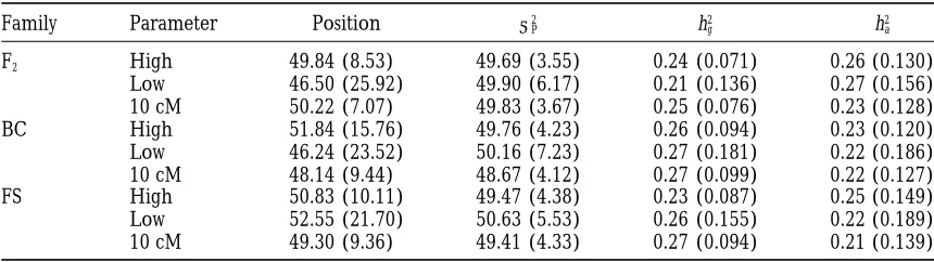
Estimates of QTL parameters with high (or low) marker informativeness and a 10-cM marker interval
Family Parameter Position s2
P h2g h2a
F2 High 49.84 (8.53) 49.69 (3.55) 0.24 (0.071) 0.26 (0.130)
Low 46.50 (25.92) 49.90 (6.17) 0.21 (0.136) 0.27 (0.156)
10 cM 50.22 (7.07) 49.83 (3.67) 0.25 (0.076) 0.23 (0.128)
BC High 51.84 (15.76) 49.76 (4.23) 0.26 (0.094) 0.23 (0.120)
Low 46.24 (23.52) 50.16 (7.23) 0.27 (0.181) 0.22 (0.186)
10 cM 48.14 (9.44) 48.67 (4.12) 0.27 (0.099) 0.22 (0.127)
FS High 50.83 (10.11) 49.47 (4.38) 0.23 (0.087) 0.25 (0.149)
Low 52.55 (21.70) 50.63 (5.53) 0.26 (0.155) 0.22 (0.189)
10 cM 49.30 (9.36) 49.41 (4.33) 0.27 (0.094) 0.21 (0.139)
See Table 1 for the standard setting. Each additional run differs from the standard setting by the parameter change noted in the second column. Standard deviations among 100 replicates are given in parentheses.
equivalent, we conclude that QTL mapping using F2 estimated QTL position. As expected, a higher QTL
effect or higher marker informativeness decreases the families has a higher power than BC and FS families
under the standard parameter setting. standard deviation of the estimated QTL position (Ta-bles 2 and 3). However, the levels of QTL heritability Under the standard setting, the QTL position and
the total phenotypic variance are successfully estimated, or marker informativeness have a smaller effect on the precision of the phenotypic variance and estimated heri-while the sum of the heritabilities, h2
g1h2a, is as expected
for all three mating designs, implying a fair partitioning tabilities. Higher marker informativeness tends to de-crease the standard deviation of various ML estimates, of the genetic and residual variances (Table 1). In
addi-tion, F2families provide more accurate estimates than while a decrease in marker informativeness leads to an
increase in the confounding of h2
g and h2a. In contrast,
BC and FS families in the estimated QTL position and
various variance components. higher heritability levels tend to be associated with a slightly larger standard deviation in the estimated phe-The levels of the QTL effect (proportional to the
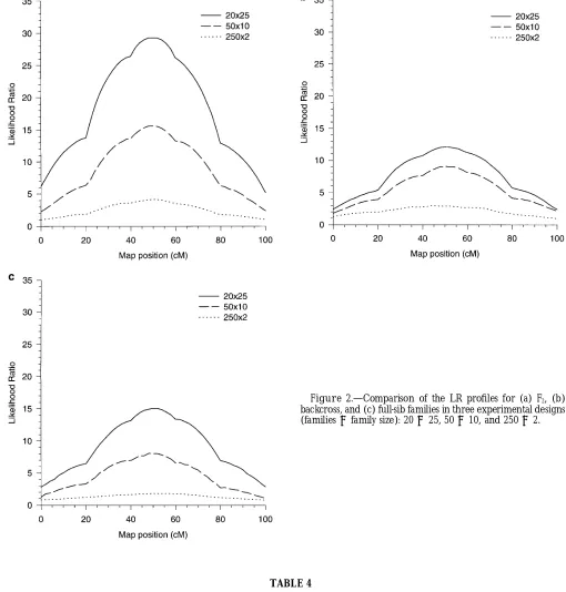
heritability value at the QTL) and marker informa- notypic variance and heritabilities.
backcross, and (c) full-sib families in three experimental designs (families3family size): 20325, 50310, and 25032.
TABLE 4
Estimates of QTL parameters under different experimental designs
Family Designa Position s2
P h2g h2a
F2 20325 48.92 (10.24) 48.94 (4.92) 0.23 (0.085) 0.24 (0.190)
25032 48.57 (22.41) 49.84 (2.95) 0.30 (0.120) 0.20 (0.148)
50032 49.16 (18.54) 50.15 (2.15) 0.26 (0.087) 0.24 (0.103)
BC 20325 49.72 (13.10) 48.76 (5.59) 0.25 (0.111) 0.22 (0.155)
25032 49.80 (27.54) 49.70 (3.39) 0.32 (0.152) 0.18 (0.160)
50032 51.64 (22.78) 50.24 (2.04) 0.30 (0.130) 0.20 (0.133)
DS 20325 50.28 (11.64) 48.88 (5.30) 0.26 (0.093) 0.20 (0.165)
25032 50.09 (29.93) 49.88 (3.48) 0.30 (0.192) 0.20 (0.212)
50032 47.47 (28.47) 49.81 (2.18) 0.25 (0.178) 0.25 (0.195)
See Table 1 for the standard setting. Each additional run differs from the standard setting by the parameter change noted in the second column. Standard deviations among 100 replicates are given in parentheses.
1144 C. Xie, D. D. G. Gessler and S. Xu
TABLE 6
Observed 95th percentile likelihood ratios under the hypothesis of no QTL segregation
Case F2 Backcross Full-sib
Standard 4.97 4.88 5.00
h2
a50.75a 5.76 5.18 5.89
h2
a50.35a 5.40 4.83 5.54
Marker informativeness:
High 5.75 5.22 5.72
Low 5.29 4.88 4.58
10-cM interval 4.19 4.19 4.63
500 families32 sibs 5.13 5.88 5.52
See Table 1 for the standard setting. Each additional run differs from the standard setting by the parameter change noted in the first column.
ah2 g 50.
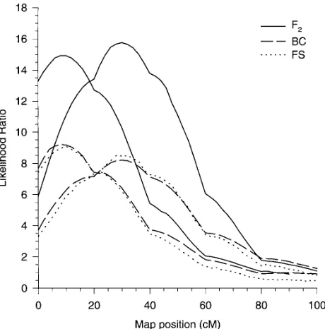
cM. It is generated by taking the average value at each position, and this method shows no bias in predicting the position of the QTL. Alternatively, taking the aver-Figure3.—Comparison of the LR profiles for F2, backcross
(BC), and full-sib (FS) families. All other information is the age maximum value of each run produces a slight bias
same as that in Figure 1 except that a single QTL is located toward the center of the chromosome, as reported in at 10 cM for the left set of curves and at 30 cM for the right Table 5. Of the three populations, the BC population set of curves.
has the largest bias in the estimated QTL position. This bias is caused by some runs where the QTL effect is not significant. In these situations, the QTL position, on average, tends to be close to the center.
large sibship per family has a pronounced effect on the
ability to detect the QTL. Figure 2 presents the results The empirical threshold values of LR test statistics over 1000 replicated simulations are reported in Table of sibships for three mating populations. The signal at
the QTL with 10 or 25 sibs per family is 250 or 500% 6. It can be seen that all three mating populations have nearly equivalent critical values. The average LR test higher, respectively, than that for two sibs per family.
In addition, with a fixed number of 500 individuals statistics and the power estimates (Type I error rate at
a 50.05) over 100 replicated simulations are summa-tested, increasing family size from 2 to 25 decreases the
standard deviation of the estimated QTL position. It rized in Table 7. First, the average LR in F2 families is
notably greater than that in BC or FS families, whereas also increases the ability to separate the genetic variance
into the polygenic and the QTL components (Tables 1 both BC and FS families have similar test statistics and powers. Second, under the condition of low marker and 4). The standard deviation of the estimated
pheno-typic variance increases as the number of families de- informativeness, FS families have a power in QTL detec-tion relatively higher than that of either F2or BC
fami-creases (Table 4).
Figure 3 shows the simulation results with the QTL lies. Recall that an F2family is generated from a single
parent by selfing. Accordingly, only two alleles at a spe-at position 10 or 30 of a chromosome of length 100
TABLE 5
Estimates of QTL parameters with the QTL located at position 10 or 30 cM
True Estimated
Family position position s2
P h2g h2a
F2 10 13.96 (18.56) 49.12 (3.44) 0.23 (0.084) 0.26 (0.125)
30 31.78 (11.19) 50.77 (4.16) 0.24 (0.086) 0.24 (0.136)
BC 10 17.90 (18.43) 49.42 (4.12) 0.27 (0.107) 0.22 (0.141)
30 36.25 (20.08) 49.83 (4.75) 0.26 (0.109) 0.23 (0.135)
FS 10 14.75 (16.17) 50.13 (4.20) 0.28 (0.101) 0.21 (0.159)
30 31.58 (13.26) 49.87 (3.72) 0.27 (0.107) 0.20 (0.153)
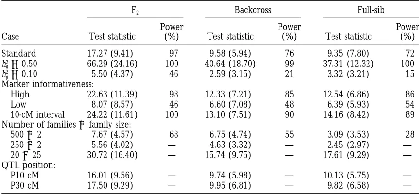
TABLE 7
Test statistic and power to detect QTLs
F2 Backcross Full-sib
Power Power Power
Case Test statistic (%) Test statistic (%) Test statistic (%)
Standard 17.27 (9.41) 97 9.58 (5.94) 76 9.35 (7.80) 72
h2
g50.50 66.29 (24.16) 100 40.64 (18.70) 99 37.31 (12.32) 100
h2
g50.10 5.50 (4.37) 46 2.59 (3.15) 21 3.32 (3.21) 15
Marker informativeness:
High 22.63 (11.39) 98 12.33 (7.21) 85 12.54 (6.86) 86
Low 8.07 (8.57) 46 6.60 (7.08) 48 6.39 (5.93) 54
10-cM interval 24.22 (11.61) 100 13.10 (7.51) 90 14.16 (8.42) 89
Number of families3family size:
50032 7.67 (4.57) 68 6.75 (4.74) 55 3.09 (3.53) 28
25032 5.56 (4.02) — 4.63 (3.32) — 2.45 (2.97) —
20325 30.72 (16.40) — 15.74 (9.75) — 17.61 (9.29) —
QTL position:
P10 cM 16.01 (9.56) — 9.74 (5.98) — 10.13 (5.75) —
P30 cM 17.50 (9.29) — 9.95 (6.81) — 9.82 (6.58) —
See Table 1 for the standard setting. Each additional run differs from the standard setting by the parameter change noted in the first column.
— Simulations are not performed under the hypothesis of no QTL segregation of these schemes.
cific locus are randomly sampled from the reference component (genetic drift) and decreases the standard deviation for the within-family component. When the population. The two alleles have a large probability
be-ing the same state under the condition of low marker increase is greater than the decrease, the net effect on the estimated phenotypic variance is an increased informativeness. In contrast, to generate FS families, two
parents or four alleles at a specific locus are randomly standard deviation.
To make the most efficient use of marker data, many sampled. This process essentially reduces the chance
of a locus being monomorphic and thus increases the QTL mapping experiments are designed to detect a number of economic traits, rather than only one trait marker and QTL informativeness. This explains why the
FS design is more powerful than the F2 and BC when (e.g.,Edwardset al. 1987). How to select parental lines
that are fixed for alternative QTLs for multiple traits is the marker information content is low.
a difficult task. The natural choice is to use more than two parental lines in a mating design. Limited
investiga-DISCUSSION
tions have shown that QTL mapping by using multiple line crosses has several advantages. First, it can handle What contributes to the variance in the estimate of
the total phenotypic variances2
P? For example, in Table multiple alleles at any locus and thus has a wider
statisti-cal inference space than a single line cross. Second, the 2 the standard deviation is higher for the high
heritabil-ity—something counter to expectation. This is due to a use of mating designs with an increased number of parents is more efficient than the use of only one F2
-scaling effect, i.e., the standard deviation being positively
correlated with the mean. The phenotypic variance is like FS family in outbred populations. This is because the variance attributable to the QTL is better estimated estimated bys2
P5 s2a1 s2g1 s2e, and thus is the sum of
three random variables. Because of the relation V 5 as the number of parents increases (Muranty1996). However, with a fixed number of individuals, there is As2
a 1 Ps2g 1 Is2e, the variance in estimates of s2g is
greater than that for s2
e. This is due in part to a con- an optimal allocation between the number of families
and the number of individuals per family where QTL founding betweens2
gands2agreater than that between s2
gands2e. This means that the variance ins2Pincreases mapping reaches its maximum power and minimum
estimation error (Soller and Genizi 1978). Third, a with s2
g, rendering a standard deviation for h2 5 0.5
higher than that for h250.10. joint test for multiple line crosses is more powerful than
a test considering crosses independently (Rebai and Similarly, in Table 4 small families have smaller
stan-dard deviations. Note that the phenotypic variance can Goffinet1993).
For convenience of presentation, the consensus be partitioned into variance between families and
vari-ance within families. When the total number of individu- method of QTL mapping described above assumes that a dominance effect is absent. We now discuss how to als is fixed, reducing the number of families increases
1146 C. Xie, D. D. G. Gessler and S. Xu
Edwards, M. D., C. W. StruberandJ. F. Wendel, 1987 Molecular
The model can be described byyj⫽ ⫹gj⫹ ␦j⫹s⫹
marker-facilitated investigations of quantitative trait loci in maize.
ej, where ␦j is the dominance deviation of a putative I. Number, distribution, and types of gene action. Genetics116:
QTL with mean 0 and variance 2
␦ and s is a family- 113–125.
Falconer, D. S.,and T. F. C.Mackay, 1996 Introduction to
Quantita-specific effect distributed asN(0,2
s). Note that2s
con-tive Genetics, Ed. 4, Longman, NY.
sists of a portion of the additive polygenic variance and Fulker, D. W., S. S. Chernyand L. R.Cardon, 1995 Multipoint dominance variance (Xu 1996b). The covariance be- interval mapping of quantitative trait loci using sib pairs. Am. J.
Hum. Genet.56:1224–1233. tweenyiandyjis Cov(yi,yj)⫽ ij2g⫹ ⌬ij2␦⫹ 2s, where
Gessler, D. D. G.,andS. Xu, 1996 Using the expectation or the
⌬ijis a descent measure indicating whetheriandjshare distribution of the identity by descent for mapping quantitative
both alleles IBD (Harris1964;Cockerham1983). The trait loci under the random model. Am. J. Hum. Genet. 59: 1382–1390.
coefficient of the dominance variance (⌬ij) is
deter-Goldgar, D. E.,1990 Multipoint analysis of human quantitative
mined by⌬jj⫽1 and genetic variation. Am. J. Hum. Genet.47:957–967.
Haley, C. S.,andS. A. Knott,1992 A simple regression method
for mapping quantitative trait loci in line crosses using flanking
⌬ij ⫽
1 forQQ-QQ,Qq-Qq-orqq-qq
0 otherwise . markers. Heredity69:315–324.
Harris, D. L.,1964 Genotypic covariances between inbred relatives. Genetics50:1319–1348.
The conditional expectation of ⌬ij given the marker Haseman, J. K.,andR. C. Elston, 1972 The investigation of linkage between a quantitative trait and a marker locus. Behav. Genet. information is computed using⌬ˆij⫽E(⌬ij|IM)⫽pi2pj2⫹
2:3–19.
pi1pj1⫹pi0pj0. In our simulation experiments we consider Jansen, R. C.,1993 Interval mapping of multiple quantitative trait
only additive effects at the QTL. loci. Genetics135:205–211.
Jiang, C.,andZ. B. Zeng,1996 Multiple trait analysis of genetic
In this study, we have used a random model
methodol-mapping for quantitative trait loci. Genetics140:1111–1127. ogy to detect a QTL. Essentially, the theoretical basis
Kempthorne, O.,1955 The correlation between relatives in inbred
of the random model is based on the variability of the populations. Genetics40:681–691.
Kruglyak, L.,andE. S. Lander, 1995 Complete multipoint
sib-IBD proportion shared by sibs at the putative QTL. For
pair analysis of qualitative and quantitative traits. Am. J. Hum. example, the variance of the IBD proportions are, on
Genet.57:439–454.
average, 1/8 for noninbred full sibs and 3/16 for sib- Lander, E. S.,andD. Botstein,1989 Mapping Mendelian factors underlying quantitative traits using RFLP linkage maps. Genetics lings from a BC. In contrast, the variance of the IBD
121:185–199. proportion is 1/4 for siblings from F2. This difference
Lincoln, S. E., M. J. DalyandE. S. Lander,1993 Mapping Genes
results in QTL mapping using F2 families being more Controlling Quantitative Traits Using MAPMAKER/QTL Version 1.1:
powerful than BC or FS families, while both BC and FS A Tutorial and Reference Manual. Whitehead Institute, Cambridge, MA.
families have similar test statistics and powers.
Male´cot, G., 1948 Les mathe´matiques de l’he´re´dite´. Masson et Cie, The F2and BC mating designs require the availability Paris.
of inbred lines. If no such lines exist in nature, one Marti´nez, O.,andR. N. Curnow, 1992 Estimating the locations and the sizes of the effects of quantitative trait loci using flanking must develop such lines, and this is costly and time
markers. Theor. Appl. Genet.85:480–488.
consuming. In this case, the FS mating design is more Muranty, H.,1996 Power of tests for quantitative trait loci detection preferable than F2and BC. In self-incompatible organ- using full-sib families in different schemes. Heredity76:156–165.
Olson, J. M.,1995 Robust multipoint linkage analysis: an extension isms, the FS mating design is the only choice.
of the Haseman-Elston method. Genet. Epidemiol.12:177–193. The consensus QTL mapping proposed here is a gen- Rebai, A.,andB. Goffinet,1993 Power of tests for QTL detection eral approach for combining or updating data. By set- using replicated progenies derived from a diallel cross. Theor.
Appl. Genet.86:1014–1022. ting the relevant⌸andAmatrices on a family-by-family
Soller, M., andA. Genizi, 1978 The efficiency of experimental
basis, families from all types of mating designs can be designs for the detection of linkage between a marker locus and sampled at different locations or different laboratories a locus affecting a quantitative trait in segregating populations.
Biometrics34:47–55. may be combined. Alternatively, data can be combined
Tinker, N. A.,andD. E. Mather,1995 MQTL: Software for Simplified
vertically; that is, data collected in the same laboratory Composite Interval Mapping of QTL in Multiple Environments. J. but at different times can be pooled through the consen- Quant. Trait Loci 1 (on line). WWW: http://probe.nalusda.
gov:8000/otherdocs/jqtl/jqtl1995-02/jqtl16r2.html. sus mapping strategy.
Van Ooijen, J. W.,andC. Maliepaard, 1996 MapQTL Version 3.0:
This research was supported by the National Institutes of Health Software for the Calculation of QTL Positions on Genetic Maps.Plant Grant GM-55321-01 and the United States Department of Agriculture Genome IV. San Diego, CA.
Xu, S.,1996a Mapping quantitative trait loci using four-way cross. National Research Initiative Competitive Grants Program
97-35205-Genet. Res.68:175–181. 5075 to S.X.
Xu, S., 1996b Computation of the full likelihood function for esti-mating variance at a quantitative trait locus. Genetics144:1951– 1960.
Xu, S., and W. R.Atchley, 1995 A random model approach to interval mapping of quantitative trait loci. Genetics141:1189–
LITERATURE CITED
1197.
Basten, C. J., B. S. Weirand Z. B.Zeng,1997 QTL Cartographer. Zeng, Z. B.,1994 Precision mapping of quantitative trait loci.
Genet-Version 1.12, North Carolina State University, Raleigh, NC. ics136:1457–1468. Cockerham, C. C.,1983 Covariances of relatives from