Investigation of the Effect of Partial Heating in an Internally Heated Vertical Annulus

(1)

ISSN(Online): 2319-8753 ISSN (Print): 2347-6710

I

nternational

J

ournal of

I

nnovative

R

esearch in

S

cience,

E

ngineering and

T

echnology

(An ISO 3297: 2007 Certified Organization)

Vol. 4, Issue 5, May 2015

Investigation of the Effect of Partial Heating

in an Internally Heated Vertical Annulus

Shahid Husain

1

, Jawed Mustafa

2

and M Altamush Siddiqui

3

Research Scholar, Department of Mechanical Engineering, Zakir Husain College of Engineering and Technology,

A.M.U, Aligarh,U.P, India1

Guest Faculty, Department of Mechanical Engineering, Zakir Husain College of Engineering and Technology,

A.M.U, Aligarh,U.P, India2

Professor, Department of Mechanical Engineering, Zakir Husain College of Engineering and Technology,

A.M.U, Aligarh, U.P, India3

ABSTRACT: Numerical Analysis has been carried out for transient two dimensional heat transfer and fluid flow during natural convection of a fixed Prandtl number (0.71) fluid through an internally heated vertical annulus. The governing continuity, Navier stokes and energy equations have been solved using finite volume SIMPLER technique. The governing equations are solved on a staggered mesh. The solutions are obtained for an aspect ratio of 10 and radius ratio of 2 by varying the heating length from full to 50%. The MPI parallel programming technique was used for domain decomposition and parallelization of code. The transient behavior of the system has been discussed in detail.

KEYWORDS: Annulus, Natural Convection, Partial heating, SIMPLER, Transient.

I. INTRODUCTION

The buoyancy induced flow occurs in geophysical, astrophysical and environmental phenomena and is also made use of in solar energy devices, thermo-siphons, nuclear reactors and in the cooling of electronic equipments and turbine blades.In the last few decades, significant interest has been shown on the modelling and control of thermal convection loops. The absence of moving components drastically reduces the probability of a failure in the removal of heat from the source. Infact, this is the main reason why natural convection is preferred to forced convection in Nuclear energy plants where safety is a primary requirement. The refrigeration of reactors in nuclear power plants and electrical machine rotor cooling therefore represent the main applications of closed-loop thermosyphon. Some important applications in which closed-loop thermosyphons are preferred to forced circulation loops are those in which the absence of pumping elements allows a considerable cost reduction, like in geothermal plants or solar heaters that have low-temperature thermal sources but a relatively high circulating flow rate or, finally, where the pumping system cannot be conveniently positioned, as incooling systems for internal combustion engines, turbine blade cooling or computer cooling. The natural convection heat transfer in vertical annuli has also a wide application in the field of engineering. The annulus represents a common geometry employed in a variety of heat transfer systems, ranging from a simple heat exchanger to the most complicated nuclear reactors[Sankar and Younghae (2010)].

(2)

I

nternational

J

ournal of

I

nnovative

R

esearch in

S

cience,

E

ngineering and

T

echnology

Vol. 4, Issue 5, May 2015

Shaarawi and Al-Aattas (1992) developed a finite-difference scheme for solving the boundary layer equations during the unsteady laminar free convection flow in open ended vertical concentric annuli. The Numerical results for a fluid of Pr= 0.7 in an annulus of radius ratio 0.5 were presented showing the developing velocity and pressure fields with respect to space and time. Sankar [2008] performed a numerical study of laminar double-diffusive natural convection in an open ended vertical cylindrical annulus with unheated entry and unheated exit.Sankar [2008] solved the steady continuity, momentum and energy equations using finite difference technique.Sankar in his study considered uniform wall temperatures, uniform wall concentration, uniform heat flux and uniform mass flux on both boundaries. The results show that there is a severe effect of the unheated entry and exit on the heat and mass transfer rates. Sankar and Younghae [2010] investigated the effect of discrete heating on convection heat transfer in a vertical cylindrical annulus. The numerical results show that the heat transfer rate was always higher at the bottom heater, which increases with the radii ratio and decreases with the aspect ratio. Venkata Reddy and Narasimham [2008] performed a numerical study of the conjugate natural convection in a vertical annulus with a centrally located vertical heat generating rod. The formulation in primitive form is solved using a pressure-correction algorithm. The average Nusselt numbers on the inner and outer boundaries show an increasing trend with the Grashof number. Wang et al. [2012] developed a finite volume model and analyzed transient natural convection in closed ended vertical annuli, with isothermally heated (or cooled) inner surface and insulated horizontal and outer surfaces. Lopez et al. [2012] performed finite difference numerical analysis of Natural convection in a closed ended annulus with a discrete heat source on the inner cylinder while the outer cylinder is cooled isothermally; the top and bottom walls and unheated portion of the inner cylinder are assumed as insulated.

The present numerical analysis solves the unsteady continuity, momentum and energy equations using finite volume method and deals with transient aspects of the flow. The study considers open ended annulus of aspect ratio 10 and radius ratio 2, the annulus being full heated and partial heated. When the annulus is considered as partially heated, the middle length is heated while the entrance and exit are unheated. The annulus being heated 98% of the total length means there is 0.01L (x=1%) unheated portion at the entrance and 0.01L unheated portion at the exit. Similarly, for 90% heated length, there will be 0.05L (x=5%) at the entrance and 0.05L at the exit that will be unheated, and so on.

II. FORMULATIONANDSOLUTION

Since, the flow is in annulus a cylindrical coordinate system, as shown in Fig. 1, is selected.The changes in properties are not significant so constant fluid properties with negligible viscous dissipation are used in the analysis. The variation of density is taken into account only in the body forces (Boussinesq approximation). Following are the non-dimensional parameters:

2

1

, , , , , ,

r z b b b

R Z U u W w t P p

b b b

 

   

             _{ }  _{ }  _ _ _{  }_{ }

        





4

,

a

T T gqb

Ra

qb k k

    

_ _  

 

 

 The governing equations after applying non-dimensional parameters will be





1

0

RU W R R Z

  



 

 _ _ _

 

 _   _

2

2 2 1

U U U P U U U U W Pr R

R Z R R R R R Z



 

 _  _  _{ } _    _ _               

2

1

W W W P W W

U W RaPr Pr R

R Z Z  R R R Z



 

 _  _  _{ } _ _    _

   

          

1

U W R

R Z R R R Z Z

    



 _  _  _    _   

   

         

The boundary conditions are:

ri : 0 1

Inner heated wall at R U W and

b R



    





ri : 0 0

Inner unheated walls at R U W and

b R



   

 

ro: 0 0

Outer adiabatic wall at R U W and

b R



   

(3)

I

nternational

J

ournal of

I

nnovative

R

esearch in

S

cience,

E

ngineering and

T

echnology

Vol. 4, Issue 5, May 2015

0 : U W 0 0

Inflow at Z and

Z Z

 

   

  

2

L: U W 0 0

Outflow at Z and

b Z Z Z

  

   

  



The model equations are nonlinear and could not be integrated exactly, so the system of equations are solved numerically by using Finite Volume SIMPLER technique. An implicit formulation is used and the resultant equation so formed is solved by Thomas algorithm. The first step in the finite volume method is to divide the domain into discrete control volumes. The boundaries (or faces) of control volumes are positioned mid-way between the adjacent nodes. Thus each node is surrounded by a control volume or cell. It is common practice to set up control volumes near the edge of the domain in such a way that the physical boundaries coincide with the control volume boundaries.

A general nodal point is identified by P as shown in Fig.2 and its neighbour’s in a two-dimensional geometry. The nodes to the west, east, north and South are identified by W, E, N and S respectively. The west side face of the control volume is referred as 'w' and the east side control volume face by ‘e'. The north side face of the control volume is referred as 'n' and the south side control volume face by ‘s’. The distances between the nodes W-P, P-E, P-N andP-S are identified byδXPW, δXPE, δYPN and δYPSrespectively. Similarly the distance of point P from face w, face e, face n

and face s are denoted by δXPw, δXPe, δY and δYPn Psrespectively. Thus the control volume dimensions, in Fig.2 are identified. In the present case a control volume based finite difference method is used. The hybrid scheme, which is a three line approximation of exact solution curve has been chosen because of its simplicity.

U W

=0, =0 , 0

Z Z

 

 

 

1 R

 _{ } 

Fig.1 Schematic diagram showing x% unheated length at entry and exit with boundary conditions

0 R

 _ 

2 2

U W

0, =0 , 0

Z Z Z

 _   _

  

xL

h

L  (1 2x) L

xL

P e

E N

W

S w

n

s

X



Y



Pw

X

 XPe

PW X

 XPE

PS Y



PN

Y



Ps

Y 

Pn

Y



w e

s n

Fig.2 Control Volume with general nodal point P

The 2D- discretization equation for a general variable ∅ can be written as.

p p E E W W N N S S

a a  a  a  a b

Where, E is east, W is west, N is north and S is south.



e w

 

n s



W S p

p E N F F F F S

a a a a a      V

1

, ( , 0

2

E e e e

a max_F D  F _

 

,

1

, ( , 0

2

W w w w

a max_F D  F _

 

,

1

, ( , 0

2

N n n n

a max_F D  F _

 

and

1

, ( , 0

2

S s s s

a max_F D  F _

 

c

(4)

I

nternational

J

ournal of

I

nnovative

R

esearch in

S

cience,

E

ngineering and

T

echnology

Vol. 4, Issue 5, May 2015

For unsteady flows, implicit discretization will be

0 0

p p W E S N P p p

V

a a a a a a S and a C

t



      





The neighbouring coefficients can be found as given in Table I.

TABLEI CONVECTIONANDDIFFUSIONTERMS Face

W E S N

Convective Term

 

u wArw

 

u eAre

 

u sArs

 

u nArn

Diffusion Term

Γ_w _w

wp

Ar z



Γ_e _e

ep

Ar z



Γ_s _s

ps

Ar r



Γ_n _n

np

Ar r



After discretization, a sequence of steps is followed for solving the equations simultaneously.The procedure involves making a guess of the pressure field and solving the momentum equation to get the pseudo velocities. Using the pseudo velocities, pressure equation is solved to get the pressure field. Then this pressure field is used to solve the momentum equation to obtain velocities. After this pressure correction equation is used to get the correction pressure, and velocities are corrected. Then the energy equation is solved and convergence is checked. The process is repeated till a satisfactory convergence is achieved. The process is repeated for each time step. The details of this method is available in [1].

The present numerical results are compared with benchmark solutions of Kumar and Kalam (1991) available in the literature for the annular cavity. The overall heat transfer rate across the cavity is given by the average Nusselt number,

defined at the hot wall as

0 L

Nu



NudZwhere

0 R Nu

R





  

 is the local Nusselt number. Comparison of the average Nusselt number, obtained in the present analysis, with those of Kumar and Kalam (1991) and Sankar et al (2011) are presented in Table II. In the low Rayleigh number range the results are in good agreement. This validates the computer code used in the present analysis.

The initial conditions set for solving the equations are constant temperature and zero velocity and zero pressure at all nodal points. The Thermal boundary conditions are constant heat flux at the heated wall while the outer wall and the unheated wallsare assumed to be adiabatic. The inlet temperature is constant and at outlet Neumann condition is used. Flow boundary conditions include no slip condition at the walls and Neumann boundary conditions at the inlet and the exit.

TABLEIICOMPARISON OF NUSSELT NUMBERS WITH OTHERS

Rayleigh No.

Present Study

Kumar and Kalam [1991]

Sankar et al. [2011]

104 3.301 3.304 3.306

105 6.303 6.268 6.269

106 _12.412 _11.888 _11.893

III.RESULTS AND DISCUSSION

(5)

I

nternational

J

ournal of

I

nnovative

R

esearch in

S

cience,

E

ngineering and

T

echnology

Vol. 4, Issue 5, May 2015

annulus and Temperature, axial and radial velocities at inlet, mid-height and exit along the radial direction are discussed for different heating lengths of the annulus.

1. Temperature, pressure and axial velocity along the annulus at different times until steady state

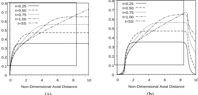
Figure 3 shows the development of temperature profile in axial direction for fully heated and 80% centrally heated annulus. Initiallythe temperature is almost constant in the heated section of the annulus.As time elapses, the constant temperature decreases attaining a linear trend during the steady state. Near the entrance the temperature is initially high but decreases with time because initially conduction dominates the convection until the flow becomes fully developed. The effect of unheated (adiabatic) entrance and exit can be seen in the Fig. 3(b).

(a) (b)

Fig. 3 Non-dimensional Temperature profile along the annulus (a) fully heated (b) 80% centrally heated (Top and bottom 10% unheated)

There is temperature rise only when heating starts at the bottom of the annulus. At the exit there is drastic fall in temperature due to unheated portion. At steady state it becomes linear in the heated region.The pressure profile in the axial direction with time until steady state is shown in Fig. 4. In the fully heated annulus (Fig 4a) the pressure at the entrance decreases, reaches to a minima and then decreases. As time elapses the negative pressure decreases and minima shifts upward in the annulus. In the 50% centrally heated annulus (Fig. 4b) , initially pressure decreases in the exit 25% unheated length, but at steady state attains the increasing trend in the fully heated annulus. Fig. 5 shows variation of temperature in radial direction at mid-height. The non-dimensional temperature decreases along the radial direction. At steady state it becomes flattened near the outer adiabatic wall.

(a) (b)

Fig. 4 Non-dimensional Pressure profile along the annulus (a) fully heated (b) 50% centrally heated (Top and bottom 25% unheated)

0 0.1 0.2 0.3 0.4 0.5 0.6 0.7 0.8

0 2 4 6 8 10

Non-Dimensional Temperature

Non-Dimensional Axial Distance t=0.25

t=0.50 t=0.75 t=1.00 t=SS

0 0.1 0.2 0.3 0.4 0.5 0.6 0.7 0.8

0 2 4 6 8 10

Non-Dimensional Axial Distance t=0.25

t=0.50 t=0.75 t=1.00 t=SS

-35 -30 -25 -20 -15 -10 -5 0 5

0 1 2 3 4 5 6 7 8 9 10

Non-Dimensional Pressure

Non-Dimensional Axial Distance

t=0.25 t=0.50 t=0.75 t=1.00 t=SS

-35 -30 -25 -20 -15 -10 -5 0 5

0 1 2 3 4 5 6 7 8 9 10

(6)

I

nternational

J

ournal of

I

nnovative

R

esearch in

S

cience,

E

ngineering and

T

echnology

Vol. 4, Issue 5, May 2015

(a) (b)

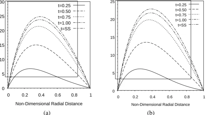
Fig. 5 Development of temperature profile in radial direction (a) fully heated (b) 80% heated

Variation of the axial velocity in radial direction with time is shown in Fig. 6. As time increases peak of the profile moves away from the heated wall until it becomes fully developed at steady state. At steady state the magnitude of the axial velocity becomes slightly less than the maximum attained value. In case of 80% heated annulus, the axial velocity decreases because the flow depends on the amount of heating.

(a) (b)

Fig. 6 Development of Velocity profile at mid-heigth in radial direction (a) fully heated (b) 80% heated

2. Transient behavior of temperature, pressure and axial velocity for different heating lengths

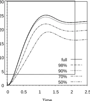
Fig. 7 shows variation of the Non-dimensional temperature with time at z=L of the heated wall. The temperature rises sharply and then decreases slightly becoming constant at steady state. As the heated length decreases, time taken to reach the peak temperature increases and the magnitude of the temperature decreases. It can be observed there is large decrease in temperature even when the heating length is 98%.Variation of axial velocity with time at exit is shown in Fig. 8.

0 0.1 0.2 0.3 0.4 0.5 0.6

0 0.2 0.4 0.6 0.8 1

Non-Dimensional Radial Distance t=0.25 t=0.50 t=0.75 t=1.00 t=SS

0 0.1 0.2 0.3 0.4 0.5 0.6

0 0.2 0.4 0.6 0.8 1

0 5 10 15 20 25 30

0 0.2 0.4 0.6 0.8 1

Non-Dimensional Axial Velocity

0 5 10 15 20 25

0 0.2 0.4 0.6 0.8 1

(7)

I

nternational

J

ournal of

I

nnovative

R

esearch in

S

cience,

E

ngineering and

T

echnology

Vol. 4, Issue 5, May 2015

Fig. 7 Variation of temperature with time at z=L (inner wall)until steady state for different lengths of heating

Fig. 8 Variation of Velocity with time at exit until steady state for different lengths of heating

As in case of temperature, also the velocity rises sharply and then decreases to become constant at steady state. As the heated length decreases the magnitude of bulk velocity leaving the annulus decreases.

Figure 9 shows the transient variation of pressure near the exit of annulus. With full heating the pressure decreases from its initial zero value and then increases slightly becoming constant at steady state. However, with decrease in the heated length, the magnitude of pressure first increases with positive valuesand then decreases, which after reaching a minimum (negative value) increases to attain constant value at the steady state. It is very interesting to see fluctuations at initial times, especially when there is partial heating. Shorter lengths of heating leads to higher fluctuations, as can be seen in the magnified Fig. 9(b). This is obvious because of low flow generation with partial heating.

(a) (b)

Fig. 9 Variation of pressure with time near the exit (a) till steady state (b) Initially

3. Steady state Pressure and temperature along the annulus

Figure 10 shows variation of pressure along the annulus at steady state. The non-dimensional pressure at the entrance decreases, reaches to a minimum value and then increases becoming zero at the exit. With decrease in the heated length there is less drop in pressure.

0 0.2 0.4 0.6 0.8 1

0 0.5 1 1.5 2 2.5

Time full

98% 90% 70% 50%

0 5 10 15 20 25 30

0 0.5 1 1.5 2 2.5

Time full 98% 90% 70% 50%

-4 -3.5 -3 -2.5 -2 -1.5 -1 -0.5 0 0.5 1 1.5

0 0.5 1 1.5 2 2.5

Time full 98% 90% 70% 50%

-0.6 -0.4 -0.2 0 0.2 0.4 0.6 0.8 1 1.2

0 0.05 0.1 0.15 0.2 0.25 0.3 0.35 0.4 0.45 0.5

Time full

(8)

I

nternational

J

ournal of

I

nnovative

R

esearch in

S

cience,

E

ngineering and

T

echnology

Vol. 4, Issue 5, May 2015

Fig. 10 Pressure profile along the annulus for different heated lengths

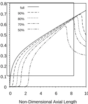
Fig. 11 Temperature profile along the annulus for different heated lengths

Figure 11 shows variation of the wall temperature along the annulus. The dimensionless temperature remains zero in unheated entrance zone, rises steeply when heated and then falls down in the unheated exit zone. The magnitude of temperature decreases with decrease in the heated length.

(a) (b)

Fig. 12 Temperature profile in radial direction for different heated lengths (a) mid-height (b) outlet

4. Steady state axial and radial velocities and temperature in radial direction

Figure 12 shows variation of the fluid temperature from the inner wall to the adiabatic outer wall.At mid height (Fig. 12a) the temperature decreases and become constant at the outer adiabatic wall. Decrease in the heated length results in low temperatures.

-25 -20 -15 -10 -5 0

0 1 2 3 4 5 6 7 8 9 10

Non-Dimensional Axial Length full

90% 80% 70% 50%

0 0.1 0.2 0.3 0.4 0.5 0.6 0.7 0.8

0 2 4 6 8 10

Non-Dimensional Axial Length full

90% 80% 70% 50%

0.05 0.1 0.15 0.2 0.25 0.3 0.35 0.4 0.45 0.5 0.55

0 0.2 0.4 0.6 0.8 1

Non-Dimensional Radial Length full 90% 80% 70% 50%

0.25 0.3 0.35 0.4 0.45 0.5 0.55 0.6 0.65 0.7 0.75

0 0.2 0.4 0.6 0.8 1

(9)

I

nternational

J

ournal of

I

nnovative

R

esearch in

S

cience,

E

ngineering and

T

echnology

Vol. 4, Issue 5, May 2015

(a)

(b)

(c)

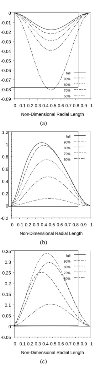
Fig. 13 Radial Velocity profile in radial direction for different heating lengths (a) mid-height (b) inlet (c) outlet

(a)

(b)

(c)

-0.09 -0.08 -0.07 -0.06 -0.05 -0.04 -0.03 -0.02 -0.01 0

0 0.1 0.2 0.3 0.4 0.5 0.6 0.7 0.8 0.9 1

Non-Dimensional Radial Velocity

-0.2 0 0.2 0.4 0.6 0.8 1 1.2

0 0.1 0.2 0.3 0.4 0.5 0.6 0.7 0.8 0.9 1

-0.05 0 0.05 0.1 0.15 0.2 0.25 0.3 0.35

0 0.1 0.2 0.3 0.4 0.5 0.6 0.7 0.8 0.9 1

0 5 10 15 20 25

0 0.2 0.4 0.6 0.8 1

Non-Dimensional Radial Length full

98% 80% 70% 60%

0 5 10 15 20 25

0 0.2 0.4 0.6 0.8 1

98% 80% 70% 60%

0 5 10 15 20 25

0 0.2 0.4 0.6 0.8 1

(10)

I

nternational

J

ournal of

I

nnovative

R

esearch in

S

cience,

E

ngineering and

T

echnology

Vol. 4, Issue 5, May 2015

Fig. 14 Axial Velocity profile in radial direction for different heating lengths(a) mid-height (b) inlet (c) outlet At the exit of the annulus, with full heating the temperature decreases from the heated wall and becomes constant at the outer wall. However, with partial heating the temperature lowers down and becomes constant throughout as shown in Fig. 12(b).Figure 13 shows variation of the radial velocity inthe radial direction at inlet, mid height and exit of the section.

At mid-height, [Fig. 13(a)] the radial velocity is negative. It decreasesfrom the inner wall, reaches to a minima and then increases up to the outer wall. This decrease in velocity increases as the heating length decreases. With full heating the radial velocity is close to zero approaching the fully developed flow region. At inlet, the radial velocity, shown in Fig. 13(b), is positive which increases from the inner wall, reaches to a maxima and then decreases up to the outer wall. This velocity decreases as the heated length decreases. At the outlet, the radial velocity shown in Fig. 13(c) again becomes positive but of lesser magnitude as at the inlet. With full heating, the radial velocity is zero showing that the flow has become fully developed. However during partial heating, radial velocity exists.

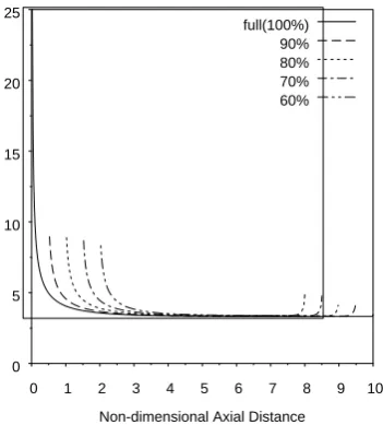
Fig. 15 Variation of Local Nusselt number for different partial heating

Fig. 16 Variation of average Nusselt number with percent heated length

Figure 14 shows variation of the axial velocity with time for different heated lenghts. At inlet, mid-height and outlet the axial vecocity is zero at inner wall increases to a maxima and then decreases becoming zero at the outer wall. As heated length decreases the magnitude of axial velocity also decreases.Figure 15 shows the variation of local nusselt number along the annulus. The local nusselt number decreases from high value at the start of heating and then becomes constant for remaining heated length. These variations in the nusselt number thus represent the developing boundary layer.

The initial high value of nusselt number is decreases with increase in unheated length although the constant value attained is same for all cases. At the point where heating ends some increase in local nusselt number is observed. Figure 16 shows the variation of average nusselt number with increase in heated length. The average nusselt decreases gradually with increase in heated length.However, the decrease in nusselt number is not very significant.

Conclusion:

The following conclusion is drawn from the results presented. With decrease in heated length

0 5 10 15 20 25

0 1 2 3 4 5 6 7 8 9 10

Nusselt Number

Non-dimensional Axial Distance full(100%) 90% 80% 70% 60%

3.50 3.60 3.70 3.80

50 60 70 80 90 100

N

u

sse

lt N

u

mb

e

r

(11)

I

nternational

J

ournal of

I

nnovative

R

esearch in

S

cience,

E

ngineering and

T

echnology

Vol. 4, Issue 5, May 2015

1) Axial velocity at outlet decreases and time taken to achieve steady state remains same. 2) Temperature at exit decreases and time taken to achieve peak value increases.

3) Fluctuations in pressure are observed near the entrance whose magnitude first increases and then decreases.

4) At mid-height the negative radial velocity increases while at inlet it decreases. 5) Average value of Nusselt number increases gradually.

NOMENCLATURE

Roman

Ar Area of control volume face A Surface area of annulus

b Annular gap (m)

Cp Specific heat (J Kg-1 K-1)

g Acceleration due to gravity (m s-2) k Thermal conductivity (W m-1K-1)

L Length (m)

p Pressure (Pascal)

P Non-dimensional Pressure q Heat flux (W m-2)

r Radial distance (m)

R Non-dimensional Radial distance

t Time (s)

T Temperature (oC) u Radial velocity (m s-1)

U Non-dimensional radial velocity w Axial velocity (m s-1)

W Non-dimensional axial velocity x Unheated length (%)

z Axial distance (m)

Z Non-dimensional axial distance Pr Prandtl Number

Ra Rayleigh Number

Greek

α Thermal diffusivity β expansion coefficient (K-1) θ Non-dimensional temperature

τ Non-dimensional time

ρ Density (Kg m-3)

ν

Kinematic Viscosity (m2 s-1)

REFERENCES

[1] S.V. Patankar, Numerical heat transfer and fluid flow, in: W.J. Minkowycz, E.M. Sparrow (Eds.), Series in Computational Methods in Mechanics and Thermal Sciences, Hemisphere Publishing Corporation/ McGraw-Hill Book Company, Washington/New York, (1980).

[2] M. A. I. El-Shaarawi and M. Khamis,, Induced flow in uniformly heated vertical annuli with rotating inner walls, Numerical Heat Transfer, vol. 12, 493-508, (1987).

[3] Ranganathan Kumar and M. A. Kalam, laminar thermal convection between vertical coaxial isothermal cylinders. Int. J. Heat Mass Transfer 34, vol. 2, 513-524, (1991).

[4] M. A. I. El-Shaarawi and M. A. Al-Attas, Unsteady natural convection in open-ended vertical concentric annuli, Int. J. Num. Meth. Heat Fluid Flow, vol. 2 503-516, (1992).

[5] P. Venkata Reddy, G.S.V.L. Narasimham, Natural convection in a vertical annulus driven by a central heat generating rod, International Journal of Heat and Mass Transfer-51, 5024–5032,(2008).

[6] M. Sankar, Numerical Study of Double Diffusive Convection in Partially Heated Vertical Open Ended Cylindrical Annulus, Advances in Applied Mathematics and Mechanics, Vol. 2, No. 6, pp. 763-783, (2010).

[7] M. Sankar and Younghae Do, Numerical simulation of free convection heat transfer in a vertical annular cavity with discrete heating, International Communications in Heat and Mass Transfer 37 600–606, (2010).

[8] M. Sankar, M. Venkatachalappa, Younghae Do, Effect of magnetic field on the buoyancy and thermocapillary driven convectionof an electrically conducting fluid in an annular enclosure, International Journal of Heat and Fluid Flow-32, 402-412,(2011).

[9] Shimin Wang, Amir Faghri and Theodore L. Bergman, Transient Natural Convection in Vertical Annuli: Numerical Modeling and HeatTransfer Correlation, Numerical Heat Transfer, Part A, 61: 823–836, (2012).