Stochastic Estimation of SRSS Method for the Structural Response due to Multi-Components of Earthquake

STOCHASTIC ESTIMATION OF SRSS METHOD FOR THE

STRUCTURAL RESPONSE DUE TO MULTI-COMPONENTS OF

EARTHQUAKE

Takashi Mochio

Professor, Dept. of Computational Systems Biology, Kinki University, Japan ([email protected])

ABSTRACT

The regulatory guide for seismic design of nuclear power plant has been vastly revised at several fields. Main items under revision are observed such as the requirement of making appropriate concern for the dynamic coupling effects of horizontal and vertical components of earthquake, and the consideration of probabilistic risk assessment against the uncertainty of earthquake.

The purpose of this paper, therefore, is to estimate the stochastic peak responses of multi-degree-of- freedom structure with closely spaced natural frequencies under the consideration of the correlations between multi components of earthquake, also aiming at reliability of SRSS method, which is occasionally used for estimation of peak responses due to multi components of input, in the field of deterministic analysis. For this target, one mathematical model for input waves is developed in order to analytically evaluate the effects of correlation between components of input, and the stochastic vibration analysis against the aforesaid input is executed based on FEM-based eigen mode analysis, transition matrix method and peak factor theory. The analytical results are compared with those by Monte Carlo simulation.

INTRODUCTION

Probability-based seismic design in consideration of multi(so-called horizontal and vertical)-components of earthquake has recently become an important research field because of increasing load level and uncertainty of earthquake, in some essential structures such as nuclear power plant. Although SRSS(Square Root of Sum of Squares) method is one of the most powerful tools to estimate the structural dynamics due to the multi-components of input, the method concerned is not frequently used in the seismic design of nuclear power facilities for the following reasons; i) several regulatory guides for load combination problems treat some dynamic effects owing to vertical input as the static design loads , ii) in the rare case where the multi-components of earthquake perform the very important role against some structural integrity, circumstantial experiments and/or detailed direct numerical calculations are regularly executed instead of estimation by SRSS method.

As mentioned before, however, SRSS is an excellent method to easily evaluate the maximum response against the multi-components of earthquake, and furthermore, because of increasing design cases due to the rising input level and growth of uncertainty, it seems that SRSS method will become important more and more in the future. Therefore, this paper stochastically evaluates the accuracy of this technique paying attention to the point of influence of the uncertainty.

MODELLING OF EARTHQUAKE WAVE

Mathematical Model of Earthquake

considers a multi-dimensional correlation of the input, the simple mathematical model is often assumed as the correlation between each component. However, the closely-spaced eigenvalue problem, where the frequency characteristics of the input carry the important role, is targeted in this research. Therefore, the model of Figure 1 where both of the frequency characteristics and the input correlation are controlled easily is introduced.

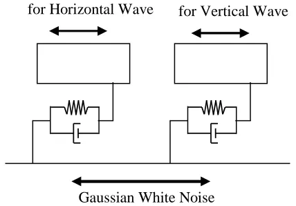
Figure 1. Analytical model for input waves

In general, the acceleration wave of an earthquake is non-white noise, and one of the secondary system such as equipment or piping is considered as the narrow band random process. Therefore, such a random process is modeled in this research by a stochastic process that has the Kanai-Tajimi spectrum. This process is obtained as an absolute acceleration of response in a single-DOF(SDOF) system subject to Gaussian white noise.

As a method of considering the correlation between multi-components of earthquake, there are;1) method of executing the stochastic analysis by introducing certain probabilistically-based mathematical model between multi-components, and 2) method of inevitably giving correlation by changing the transfer characteristics (that is, damping and natural frequency are changed) on the same support just as Figure1. This paper adopts second method for some reasons that it is easy for Figure 1 to make a realistic model when thinking about actual wave propagation, and it is extensible also in the multi-components problem of no correlation by setting non-common supports. Then, equations of motion become as follows:

(

)

(

g

)

g

g g

z w ν z

ν Ω ν Ω h ν

z w v z

v Ω v Ω h v

      

 

 

      

 

 

− = −

= +

+

− = −

= +

+

2 2 2

2 2 2 2 2 2

1 1 1

2 1 1 1 1 1

; 2

; 2

(1)

where w_p

(

p=1,2

)

denotes a narrow-band random process which has the Kanai-Tajimi spectrum, and z_g is an input acceleration modeled by Gaussian white noise.

The mathematical model which becomes an input to the structures is assumed to be given by Equation 2 as the products with stationary random process w_pand deterministic function (envelope function) to express amplitude non-stationarity a_p

(

p=1,2

)

.

( )

( ) ( )

( )

(

r t r t

)

mp

p p

p

p t a t w t a t A e p e p

z 1 2

; ~

0

−

− ₋

=

= 



 (2)

Here, a_p is selected so that its maximum value may become one, by after-mentioned reasons (standardization of input level). Parameters Ω_p,h_p

(

p=1,2

)

in Equation 1 are essentially related to

Gaussian White Noise

predominant frequency and degree of frequency band, respectively. In addition, it is shown that affixing characters 1 and 2 in Equation 1 are the amounts concerning the horizontal motion and vertical one. Scaling of Mathematical Model as Earthquake

Though it is possible to think about the input acceleration waves ~z₀₁,~z₀₂ that have various correlations by using Equation 1, in this case, the parameters _Ωp,_hp have been changed. This shows

certain possibility that the difference goes out at the levels of ~z₀₁,~z₀₂ even if the same Gaussian white noise with spectral intensity

( )

I_g is used. In other words, there is a possibility not being guaranteed for impartially evaluate at the same input level, when it makes comparative study of structural response by changing the input correlation. In order to evade such inconvenience as much as possible, some modifications by scaling shown at Equation 3 are used for the final input accelerations z₀₁,z₀₂ against structures.

2 2 2 2

2 2 02 1 1 1 2

1 1 01

2 1

, μ a w

σ w a z w a μ σ

w a z

w w

  

 

   

 



  



≡ =

≡

= (3)

Where 2

p

w

σ

 explains variance of wp. It is also noted that the transformation according to Equation 3 doesn’t influence stochastic results by introducing the correlation coefficients about the input correlation.

STOCHASTIC ESTIMATION

Equations of Motion

If absolute displacements at an arbitrary point of primary and/or secondary structures (In this paper, it is called a main structure after this.) are assumed to be

x

ˆ

_i

,

y

ˆ

_i, relative displacements

x

_i

,

y

_i become as follows:

02

01 , ˆ

ˆ z y y z

x

xi = i − i = i− (4)

In addition, because it is inconvenient to generate displacements as x,y, it is unitedly described

u

_kin which index kmeans k−th _{degree of freedom. Utilizing the relative displacement vector} X_composed

by

u

_k, total equations of motion relating to the main structure can be derived in the following form:

1 01z 2 02z

+ + = − −

MX CX KX  ME_ ME _{ (5)} where,

M C K, , ;

mass, damping and stiffness matrices for the main structure

E_p;

operating point vector of

p-direction seismic load

In Equation 5, the following mode superposition procedure is applied by using eigen modes Φ of the main structure and modal coordinate vector q.

q Φ

That is, by inserting Equation 6 into Equation 5 under the assumption of orthogonality for the damping matrix, equations of motion in modal coordinate space can be obtained as follows:

[

1

]

01

[

1

]

02

02 2 1

01 1 1

2 2

1 1

1

2 2

1 1

~ ~

2 2

z ζ ζ

z ζ ζ

z z

ω ω

ω ξ ω

ξ

T n T

n

T T

n n

n

  

  

  

 

 

 

− −

=

− −

=   

 

  

  +   

 

  

 

+ _{q M}−_{Φ ME M}−_{Φ ME}

0

0 q

0

0 q

(7)

where,

ω_j,ξ_j ; j th-order modal frequency and modal damping , M~ ; modal mass matrix , ;

2 1 j

j ζ

ζ j th-order participation factor in each component of earthquake Thus, j th-order equation of motion is separately given as

1 2

2

01 02

2

j j j j j j j j

q



+

ξ ω

q



+

ω

q

= −

ζ

z



−

ζ



z

(8)

and then,

u

_kcan be obtained by Equation 6 in the following form:

∑

=

=

n

j

j j k

k

φ

q

u

1

(9)

Stochastic Analysis of Dynamics

Combining Equations 1,3,7 and 8, the extended state space equation reads

( )

t =

( ) ( )

t t + z tg

( )

Q A Q b_{ (10)}

where,

{

1 1 2 1 1 2

}

T

n n

q q

ν ν

q q

ν ν

=      

Q

,

b=

[

0  0 −1 −1

]

T

( )

t

A

; coefficient matrix composed of

ω

_j

ξ

_j

ζ

_j

μ

_p

h

_p

Ω

_p

a

_p

( )

t

p

,

,

,

and

,

,

In this case, though z_gis stationary Gaussian white noise, the stochastic response of Qshows a non-stationary random process because of matrix Aincluding time-dependent parameter a_p

( )

t

. By the way,

non-stationary covariance matrix

W , relating to the foregoing response vector Q , satisfies the following matrix differential equation:

( )

t =

( ) ( )

t t +

( ) ( )

t T t +2

π

I_g T

W A W W A bb ₍₁₁₎

[ ]

u

E

[ ]

σ

( )

t

E

k2

=

φ

k

q

⋅

q

T

φ

kT

≡

u2_k (12)

where,

φ

_k

=

[

φ

_k1



φ

_kn

]

,

E

[ ]

⋅

; operation as ‘expected value’

Equation 12 is derived under the assumption that mean value of u_kis zero and effects by deadweight are negligible for reasons of linear system. Equation 12 can be actually calculated through Equation 11. Estimation of Maximum Response

SRSS method, in principle, is one of the deterministic technique in order to get maximum responses. Then, first of all, definition against the expectation of maximum response should be set stochastically. In this paper, the following form is adopted as definition:

( )

[

u

k

t

_Max

]

{

σ

uk

( )

t

P

uk

}

Max

E

=

×

(13)

where

k

u

P is the peak factor about σ

( )

t

k

u , and it is dependent on time exactly. Suppose , in this paper,

k

u

P may be approximately considered as independent parameter, then Equation 13 can be calculated by estimating two terms separately.

Such peak factor is presumed in the form (Kiureghian (1980))

( )

_{( )}

(

)

(

)

(

)

2 0 2 1 0 2 45 . 0 n n 1 1 ~ 69 . 0 ; ~ 69 . 0 ; ~ 38 . 0 63 . 1 l 2 5772 . 0 l 2 λ λ λ δ λ λ π ν δ ν δ ν δ ν T ν T ν P e e e uk − = =    ≥ < − = + = (14)

where

λ

_mmeans spectral moment defined as

( ) ( )

2 0

m

m

G

F

H

d

λ

=

∫

∞

ω

ω

ω

ω

(15)

and

G

_F

( )

ω

is one-sided power spectral density of input acceleration, and H

( )

ω represents frequency response function as relative displacement vs. input acceleration. Also, H

( )

ω can be obtained by utilizing Equations 1,3,8 and 9 in the following form:

( )

₍

₎

₍

₎

₍

₎

ω i s n

j s hΩ s Ω

Ω s Ω h μ ζ Ω s Ω h s Ω s Ω h μ ζ ω s ω ξ s φ ω

H j j

j j j j k = =

∑

_             + + + + + + + + + − = 1 2 2 2 2 2 2 2 2 2 2 2 2 1 1 1 2 2 1 1 1 1 1 2 2 2 2 2 2

2 (16)

Derivation of SRSS Composed by Stochastic Parameters

When a dynamic response problem due to horizontal/vertical components input is approximately solved by SRSS method, the following two kinds of calculations are thought according to an analytical level.

1) calculation method 1 (called as SRSS1)

Method of executing approximate calculation to disregard only the effects through horizontal/vertical components of input, but to consider the coupling between vibration modes. For this case, computational expression may be shown as:

( )

[

] [

2

]

2

Max V k Max H k Max

k u u

u = + (17)

where,

u_kH

; response by detailed analysis considering coupling-effects of modes due to horizontal input only

V

k

u

; response by detailed analysis considering coupling-effects of modes due to vertical input only

2) calculation method 2 (called as SRSS2)

Method of executing approximate calculation to disregard the effects through horizontal/vertical components of input and also the coupling between vibration modes. For this second case, computational expression may be shown as:

( )

[

_~

] [

2 _~

]

2

Max V k Max H k Max

k u u

u = + (18)

where, Max H k

u

~

_{; response by ordinary SRSS method , which neglects coupling between vibration modes, due to}

horizontal input only

Max V k

u

~

_{; (same as the horizontal case)}

It is possible to stochastically calculate the maximum response of relative displacement according to the above-mentioned definition, by using the probabilistic analytical method (Equation 13) developed in this study.

Evaluation of Multi-Dimensional Correlation for Input

The correlation coefficient that doesn't depend on the input level, in this paper, is used as an amount to evaluate the correlation concretely. The correlation coefficient is obtained by Equation 1 as follows:

[

]

1 2

1 2

1 2

1 2

2 2

1 2

w w w w

w w E w w

E w E w

κ

ρ

σ σ

= =

   

   

   

 

 

 

(19)

where,

[

]

[ ]

[ ]

[ ]

1 2 1 2 1 2

[ ]

1 2

2 1 2 2 2 1 2 2 1 1 2 1 2 2 2 1 2

1

w

Ω

Ω

E

ν

ν

2

h

Ω

Ω

E

ν

ν

2

h

Ω

Ω

E

ν

ν

4

h

h

Ω

Ω

E

ν

ν

w

E









=

+



+



+





[ ]

w

2

=

Ω

4

E

[ ]

ν

2

+

4

h

Ω

3

E

[ ]

ν

ν

+

4

h

2

Ω

2

E

[ ]

ν

2

;

(

p

=

1

,

2

)

NUMERICAL EXAMPLES

Model for Calculation

Although the object of this research is an arbitrary linear multi-degree-of-freedom structure, the key task in this paper is to examine the closely-spaced eigenvalue problem in consideration of the input correlation. Therefore, the following two models are fixed.

Figure 2. Two types of model for estimation

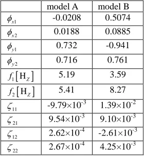
Each model in Figure 2 is composed of 18 finite beam elements, and adjusted so as to possess the closely-spaced eigenvalue or non-closely-closely-spaced eigenvalue by changing the combinations of mass and stiffness. In addition, the third eigenvalue or more are considered by setting to 40Hz or more so that the number of higher-order vibrations should not influence the dynamics coming from two lower closely-spaced frequencies, because it makes the prospect of the phenomenon easy. The modal parameters used to calculate are as shown in Table 1.

Table 1: Modal parameters of two models

model A model B

1

x

φ -0.0208 0.5074

2

x

φ 0.0188 0.0885

1

y

φ 0.732 -0.941

2

y

φ 0.716 0.761

[ ]

1 HZ

f 5.19 3.59

[ ]

2 HZ

f 5.41 8.27

11

ζ -9.79×10-3 1.39×10-2

21

ζ 9.54×10-3 9.10×10-3

12

ζ 2.62×10-4 -2.61×10-3

22

ζ 2.67×10-4 4.25×10-3

In Table 1, φ_x1 is the first-order mode at the top of the main structure in

x

direction (horizontal direction) and f1is the first-order natural frequency of the main structure. Moreover, the modal damping ratio is

assumed to be 0.02 uniformly. Some Numerical Results

6 . 0 ,

2

5 . 0 ,

3 . 0 ,

1 ,

379 . 5

1 2

2 1 1

22 21 12

11 2

1

= =

+ =

= = =

= =

= =

h Ω

ω ω Ω

r r r

r I

A

Am m g

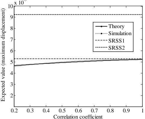
Numerical results are shown in Figures 3 and 4. Figure 3 gives the expected maximum values relating to the relative displacement in y direction at the toe point of main structure (at model A), as correlation coefficients being parameter in horizontal axis. Figure 4 shows the same results as Figure 3 excluding model type, namely this case is for model B.

0.2 0.3 0.4 0.5 0.6 0.7 0.8 0.9 1

2 3 4 5 6 7 8 9 10x 10

-5

Correlation coefficient

E

x

p

ect

ed

v

al

u

e (

m

ax

im

u

m

d

is

p

lacem

en

t)

Theory Simulation SRSS1 SRSS2

Figure 3. Expected values of maximum displacement (model A)

0.2 0.3 0.4 0.5 0.6 0.7 0.8 0.9 1

1 2 3 4x 10

-4

Correlation coefficient

E

x

p

ect

ed

v

al

u

e (

m

ax

im

u

m

d

is

p

lacem

en

t)

Theory Simulation SRSS1 SRSS2

Although the correlation between multi-components of input can be controlled by changing the values of p

Ω

and/or

h

_pat Equation 19, in this paper,

Ω

_pis fixed and only

h

_pis changed. More in detail, h₂is properly changed within the range of

(

0<h₂<h₁

)

, under the condition of

h

₁

=

0

.

6

, then the correlation coefficient is finally obtained by Equation 19.

Both Figure 3 and 4 give the numerical results derived from, the stochastic analytical method proposed in this paper (called ‘Theory’ in figure), 500 times Monte Carlo simulation (‘Simulation’), SRSS method 1 (‘SRSS1’) and SRSS method 2 (‘SRSS2’). By estimating and comparing the results, the following 4 findings are confirmed:

1) The results by analytical method and Monte Carlo simulation show a tolerable agreement, and the prospect of validity about the analytical technique is obtained.

2) For the main structure with closely-spaced frequencies, there is a possibility that some error of about 10% or less is generated in the expected maximum response by SRSS, according to the level of correlation between multi-components of input. But it is noted that the error by SRSS means over safety design.

3) For the same closely-spaced system, disregarding the coupling between vibration modes (SRSS2) causes deterioration in accuracy. But this case also implies the over safety design of SRSS method.

4) About SRSS method disregarding only the effects through horizontal/vertical components of input, (SRSS1), there is less depression of calculating accuracy.

The above findings finally suggest that SRSS is robust technique against the closely-spaced eigenvalue problem and the dynamic coupling effects of horizontal and vertical components of earthquake.

CONCLUSION

The accuracy of the SRSS method is stochastically examined by executing the probabilistic vibration analysis of a linear multi-degree-of- freedom structure with closely spaced natural frequencies under the consideration of the correlations between multi components of earthquake. On the viewpoint of stochastic phenomenon, SRSS is evaluated as a very powerful technique against not only deterministic input but also random one.

REFERENCES