Seismic soil-structure interaction of a nuclear building: Comparison of two different methods

(1)

Transactions,_SMiRT-23

Manchester, United Kingdom - August 10-14, 2015

Division V, Paper ID 248

Seismic soil-structure interaction of a nuclear building: Comparison of two

different methods

Jana Sue Bochert1, Henry Schau2and Timo Schmitt3

1_{Structural Analysis Expert, TÜV SÜD Energietechnik GmbH, Germany}

2_{Structural Analysis Division Manager, TÜV SÜD Energietechnik GmbH, Germany}

3_{Seismic Hazard and Structural Dynamic Expert, TÜV SÜD Industrie Service GmbH, Germany}

ABSTRACT

This paper presents the computation of response spectra for a nuclear building, including seismic soil-structure interaction (SSI), using two different methods. To do so, established computer programs like the SASSI computer code and ABAQUS with Infinite Elements are used. The SASSI computer code is based on the Thin Layer Method developed by Lysmer et al. (1981) as a method for computations in the fre-quency domain. The calculations here are realized with the enhanced efficient SASSI 2010 by Ostadan et al. (2012). Another method, known as the Lysmer damper and also developed by Lysmer and Kuhlemeyer in 1969, is implemented in ABAQUS and called Infinite Elements. These elements contain values for the boundary damping effect. Considering linear elastic material behavior close to the bounda-ry, both methods transmitted and absorbed all normally incoming plane body waves.

The paper then discusses the results of the response spectra obtained by the two methods. This compari-son assesses the viability of the methods. It also discusses the “accuracy” of the results in terms of effi-ciency and compares computation times and pre-processing times.

1 INTRODUCTION

1.1 Background

Nuclear buildings have to withstand earthquakes with low probabilities of exceedance. The earthquake design loads are determined in site-specific seismic hazard studies. During a strong earthquake, the build-ing and its surroundbuild-ing soil can exhibit non-linear behavior, so the non-linear site response spectra has to be calculated. For nuclear buildings, floor response spectra have to be calculated with a numerical model, taking the radiation damping and the soil-structure interaction into account. The soil-structure interaction has a significant influence on the results if the building is situated on soft soil, or, on the other hand, it has no influence if the building is built on a rigid foundation. The influence can be explained via the interac-tion of the surrounding soil with deformainterac-tions due to earthquake excitainterac-tion. This interacinterac-tion changes the response of the structure. The soil-structure interaction, which is based on wave propagation phenomena for infinity, has already been the subject of many studies. Incorporating wave propagation phenomena in a numerical model is highly complex, because the wave has to move into infinity. Normal finite element models have artificial boundaries which do not exist in reality because the soil is assumed to be infinite.

1.2 Outline of the Paper

(2)

2. HISTORY AND STATE OF THE ART

2.1 Analytical and Numerical Methods

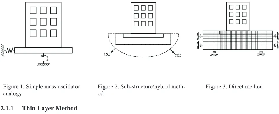
Since the last century, a lot of theories and boundary conditions have been developed to predict the soil-structure interaction. The non-complex analytical method for radiation damping due to the soil is the sim-ple mass oscillator analogy (Figure 1). There, the soil is depicted as a damper and spring. This concept was developed by Hsieh (1962) and Lysmer (1965), when Lysmer extended the frequency-dependent damping and stiffness coefficient for this model.

Numerical methods include more complex theories like the Boundary Finite Element Method (Jaswon 1963), Infinite Elements (Bettes 1992), Scaled Boundary Finite Element Method (Wolf 2000), the Thin Layer Method (Lysmer and Waas 1972), Viscous Boundaries (Lysmer and Kuhlemeyer 1969) and many more.

Furthermore, the theories are broken down into direct methods and sub-structure methods. These numeri-cal models differ in their finite element meshes and their radiation damping boundary conditions. Howev-er, even though the Thin Layer Method (see Section 2.1.2) is a sub-structure method, the continuum yields a near and a far field (Figure 2). The direct method is modeled for example with viscous dampers (Figure 3 and Section 2.1.2) or with a large element mesh for soil discretization to incorporate radiation damping.

Many theories and software applications have been developed to account for non-linear site responses and the calculation of free-field response spectra. They can be differentiated by the geometry and the kind of analysis. The most commonly used forms are 1D analyses for horizontally oriented layers with no basin effects. For more complicated geometries, 2D or 3D analyses are needed. According to the analysis, a dis-tinction can be made between equivalent-linear and non-linear analyses as well as total stresses and effec-tive stresses. Some programs offer several calculation approaches.

Figure 1. Simple mass oscillator analogy

Figure 2. Sub-structure/hybrid meth-od

Figure 3. Direct method

2.1.1 Thin Layer Method

(3)

23rd_{Conference on Structural Mechanics in Reactor Technology}

Manchester, United Kingdom - August 10-14, 2015 Division V

The transmitting boundaries are derived based on the generalized Love wave, for instance, which is de-fined here with the function _ߜ of the harmonic motion with displacement v(z), the frequency ߱, the time

step t, the wave number k , the length x

ߜ ൌ ݒሺݖሻ݁௜ሺఠ௧ି௞௫ሻ ₍₁₎

and the assumption of linear variations of displacement within each layer. The formulated eigenvalue problem (Waas 1972) in the frequency domain with the eigenvalue matrix {V} is subdivided here for in-stance into generalized Love wave motions, which depend on the sub-matrices [A], [G] and [M] of the soil:

ሺሾܣሿ݇ଶ_{൅ ሾܩሿ െ ߱}ଶ_{ሾܯሿሻሼܸሽ ൌ ͲǤ} ₍₂₎

Waas formulated the force-displacement relationship in the frequency domain for the layered system, where the displacement is {U}, {P} is the force and [R] is the dynamic stiffness:

ሼܲሽ ൌ ሾܴሿሼܷሽǤ (3)

and by using the eigenvalues and eigenvectors as well as the stress-strain relationship in each layer, the equation for the dynamic stiffness of the semi-infinite layered region can be formulated as below:

ሾܴሿ ൌ ݅ሾܣሿሾܸሿሾܭሿሾܸሿିଵ_{൅ ሾܦሿǤ} ₍₄₎

The half space is generated with layers, where the base of the half space is discretized with the Lysmer damper/viscous boundaries, which are exemplified in Section 2.1.2. For a more detailed description of the theory and the functionality of SASSI, see the Theoretical Manual for SASSI 2010.

Figure 4. Diagram of the implementation of transmitting boundaries and viscous dampers [see Towhata (2008)]

2.1.2 Viscous Boundaries

For the non-reflecting boundaries, Lysmer and Kuhlemeyer developed viscous boundaries in 1969, better known as viscous dampers for the half space (see Figure 3). The viscous boundaries make sense, because radiation damping is comparable to viscous damping. The dampers are constructed horizontally to radiate the S-wave and vertically for the P-wave direction at the boundaries of the finite mesh, and calculations can be made in the time and frequency domain. These dampers are used in the vertical direction in SASSI and for all directions for the ABAQUS model. In ABAQUS (see ABAQUS Theory Manual), these ele-ments are called Infinite Eleele-ments.

(4)

linear relationship between stress and strain, and the simplification due to Young’s modulus leads to non -frequency-dependent viscous boundaries. The viscous boundaries can be discretized as dampers for the vertical direction Cp, depending on the P-wave velocity Vp and for the horizontal direction Cs, with the

S-wave velocity Vs. Both equations depend on the density ߩ:

ܥ௣ൌ ߩܸ௣ (5)

ܥ௦ൌ ߩܸௌ (6)

2.1.3 Non-linear Site-response

DEEPSOIL (Hashash et al. 2012) was used for the calculations presented. The program can perform 1D linear-equivalent analyses in the frequency domain (SHAKE approach), as well as non-linear time do-main wave propagation analyses. The calculations presented are based on the linear-equivalent method, using frequency-dependent damping. The linear-equivalent method is appropriate for moderate earth-quake loads and shear strains. It is an iterative procedure: initially, a pure visco-elastic behavior with pa-rameters corresponding to very low strain conditions (initial stiffness and damping) is assumed for the medium. Then, preliminary strain is evaluated for each point, which is used to modify the parameters ac-cording to the reduction curves. In the next step, seismic wave propagation is calculated again taking the modified parameters into consideration. This procedure is repeated until compatibility with the strain lev-el is reached.

2.2 Computer Programs

The most-used and established computer program for SSI for nuclear installations is SASSI. Previously, the energy transmitting boundaries were implemented in FLUSH (Lysmer et al. 1975) and ALUSH (Ber-ger et al. 1975). An alternative to SASSI could be to use the direct method with viscous dampers in standard FEM programs like ANSYS or ABAQUS. Another option is to use the simple mass analogy, al-lowing spring and damping elements to be applied in commercial FEM programs. Coefficients of the springs and dampers can be obtained from ASCE (1998).

The best-known and used program for 1D site response analyses is SHAKE. It is based on the equivalent-linear approach. Other examples for 1D analyses are EERA, STRATA (Rathje and Kottke 2010), PROSHAKE and DEEPSOIL. For 2D and 3D site response analysis, special alternative programs are used.

3. DESCRIPTION OF THE NUMERICAL MODEL

3.1 General Description

(5)

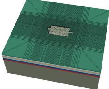
As described in Section 2.1, the soil-structure interaction has to be considered to calculate the floor re-sponse spectra, and the methods are implemented into the calculation via computer programs, in this case SASSI and ABAQUS. For these calculations, the building is generated with shell and solid elements as shown in Figure 5.

Figure 5. Finite element model of the building with the marked nodes TP (top story) and BM (basement)

The building, or rather the models used for ABAQUS and SASSI basically differ in the discretization of the half space. However, in both cases, each of the buildings has to be modeled with the same mass and of course the same material parameters. The Young’s Modulus used for the concrete is E = 33,000,000 kN/m2, the material weight is25.48 kN/m3 and the damping ratio is given in KTA 2201.3 (2013) as 7%. The S-wave velocity must be used for the element size for mesh discretization in the soil model, especial-ly for the thickness of the horizontal layers. The differences in the soil model and between the time and frequency domain calculation depend on the treatment within the SASSI and ABAQUS models. A de-tailed explanation is provided below.

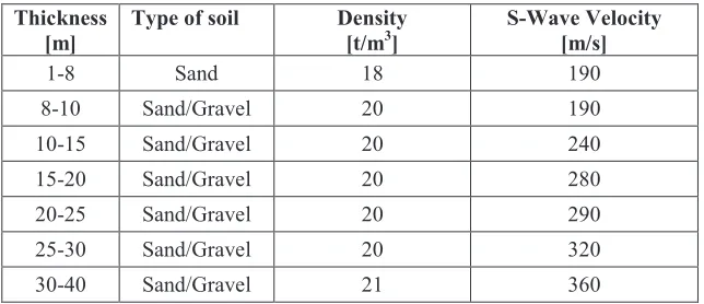
Table 1: Overview of the initial layered soil parameters

Thickness [m]

Type of soil Density [t/m3]

S-Wave Velocity [m/s]

1-8 Sand 18 190

8-10 Sand/Gravel 20 190

3.2 ABAQUS Model

The calculation is made in the time domain with the implicit method of Hilber-Hughes-Taylor time inte-gration in ABAQUS (see the ABAQUS User Manual). For the calculation in the time domain, the materi-al damping is implemented using Rayleigh damping.

(6)

Therefore, the soil model is discretized 40 m in depth, with 8 layers, and the horizontal discretization is roughly one length of the building for each site. The geometries of the Infinite Elements are also selected with the length of the building.

Figure 6: ABAQUS model: structure and soil model Figure 7: ABAQUS soil model surrounded by viscous boundaries (Infinte Elements)

To validate the soil model/the plane, the free-field response spectrum has to be calculated and compared with the DEEPSOIL free-field response spectrum (see Figure 8). However, it cannot be expected to pro-duce the same results, because ABAQUS uses a linear calculation and DEEPSOIL is based on a non-linear equivalent calculation, but a certain level of comparability should be achieved. The results of the far field response spectrum (FFRS) in Figure 6 (node: FFRS) with ABAQUS and the original spectrum with DEEPSOIL (see Figure 8) are both shown in Figure 9. The two curves are sufficiently compatible, because the first peak at 4.5 Hz is similar in ABAQUS and DEEPSOIL. Moreover, the peak accelerations are alike. Differences are apparent above 4.5 Hz, where the free-field response spectrum drops faster than the non-linear calculation. This drop in the curve continues to the higher frequency domain at approx. 10 Hz, as can be seen where the rigid body acceleration is reached.

Figure 8. Smoothed response spectra with 5 % damping at different depths

Figure 9: Comparison of free-field response spec-trum at node FFRS with 5 % damping

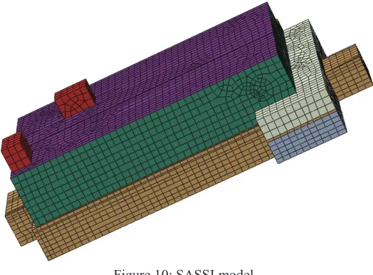
3.3 SASSI Model

(7)

Figure 10: SASSI model

The seismic input (a response spectrum-compatible time history) is located at -40 m, as it is in the ABAQUS model, too. As already described in Section 2.1.1, the calculation in SASSI is made in the fre-quency domain and f = 0.048 Hz is chosen as the frefre-quency step. The solution in the frefre-quency domain is transformed to the time domain using the Fast Fourier Transformation. Then, the floor response spectra of the building are calculated from the time histories

4. RESULTS

4.1 Acceleration Response Spectra

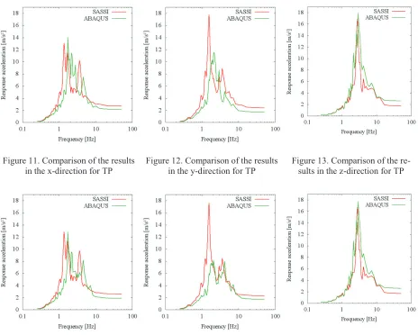
To check the results (acceleration response spectra) for plausibility, the nodes on all 4 corners for each story of the building were calculated. The results must be nearly coincident to examine the symmetry of the building. Furthermore, the maximum values of the response spectra decrease, in each story, starting from the top story. Symmetrical behavior was evaluated and the results are nearly the same for each of the 4 corner nodes. The ratio of the maximum values between the different ascending storys matches, as dis-cussed below. For the investigation of the results, two nodes, one at the corners of the top story (TP node) and one in the basement (BM node) were selected (see Figure 5). However, all response spectra in Figure 11 to Figure 16 are calculated with 2 % damping and three frequency domains are incorporated when discussing the results: the lower (1-3 Hz), middle (3-7 Hz) and high frequency domains (7-50 Hz).

(8)

Figure 12 shows differences in the y-direction, the peak for the 1st eigenfrequency calculated in SASSI is higher than the peak from ABAQUS. A good correlation is reached in the middle frequency domain, while some difference arises in the high frequency domain when determining the rigid body acceleration.

The curves in z-direction in Figure 13 show perfect compliance. Both models hit the 1st eigenfrequency at 3 Hz with a comparable value of response acceleration; a good match is also seen in the middle fre-quency domain. Only in the high frefre-quency domain are there some differences – the rigid body accelera-tion is reached at 1.8 m/s with SASSI and at 2.5 m/s with ABQUS.

The results for the selected node in the basement (BM) are shown in the figures below. It is evident that the acceleration is lower than for the top story node, fulfilling the plausibility criteria. The results the in Figures 14 - 16 replicate the phenomena of the curves on the top story (Figures 11-13). Amplitude differ-ences are also apparent in the y-direction, but with a good match in the middle frequency domain. The results in the x- and z-directions of the high frequency domain correlate well, however some differences in the ordinates are observed in the middle and the higher frequency domain. Also, the comparison shows a slight frequency shift between the ABAQUS spectrum and the SASSI spectrum for the x- and y-direction.

Figure 11. Comparison of the results in the x-direction for TP

Figure 12. Comparison of the results in the y-direction for TP

Figure 13. Comparison of the re-sults in the z-direction for TP

Figure 14. Comparison of the results in the x-direction for BM

Figure 15. Comparison of the results in the y-direction for BM

(9)

In spite of this, the compatibility of the results is excellent, especially bearing in mind that they were cal-culated using two different programs, methods (direct and sub-structure method) and calculation types (time domain and frequency domain).

4.2 Efficiency, Computation Times and Pre-processing Times

The CPU times of each model are important, especially if many model variations have to be calculated. The runtime, of course, is highly dependent on the degrees of freedoms. The number of nodes and ele-ments are much higher in the ABAQUS model than in the SASSI model. Furthermore, the calculation in time domain (ABAQUS) takes more CPU time than frequency domain calculation (SASSI). As a result, the runtime for calculation (standard PC) using SASSI is up to 10 times faster than the one with ABAQUS.

5. CONCLUSION

This paper compares results in terms of acceleration response spectra calculated with SSI models using ABAQUS and SASSI. The comparison shows that both computer programs produce similar results. Some differences in the maximum ordinates, particularly in the y-direction were observed for the example pre-sented. However, the good results are comparable, although they are obtained by different methods (direct and sub-structure method) and calculation types (time and frequency domain). The comparison of the re-sults shows that ABAQUS is an alternative to SASSI for SSI analysis. Therefore, the ABAQUS soil model used in this paper provides a basis for a wide range of alternative calculations incorporating wave propagation phenomena. Nevertheless, the ABAQUS soil model shall be adjusted or combined with site response analysis (e.g. using DEEPSOIL) to produce comparable free-field spectra. However, this calcu-lation approach is based on indefinable inaccuracies. Usually SASSI is to be preferred for this kind of analysis. Transient computations in ABAQUS incorporate the dynamic process of motion, but increase the computation time drastically. The sub-structure method, as it is implemented in SASSI, is much more efficient. Concluding, it can be stated, that ABAQUS and SASSI and the related computational methods for SSI analyses, result in comparable structural response but have significant differences in efficiency

_.

7. ACKNOWLEDGEMENT

This research was partially carried out with SASSI 2010, which was provided by Wölfel Beratende In-genieure GmbH + Co. KG, Höchberg, Germany. The authors gratefully acknowledge this support, espe-cially the help of Dr.-Ing. Fritz-Otto Henkel.

8. REFERENCE

ABAQUS (Version 6.13). Dassault Systèmes Simulia Corp., Providence, RI, USA.

ASCE (1998). Seismic Analysis of Safety-Related Nuclear Structures (4-98), American Society of Civil Engineers.

Berger, E., Lysmer, J. and Seed, H. B. (1975). “ALUSH - A Computer Program for Seismic Response Analysis of Axisymmetrical Soil-Structure Systems”, Report 75-31, University of California, Berkeley.

Bettes, P. (1992). “Infinite elements”, Penshaw, Sunderland, UK.

EERA. A Computer Program for Equivalent-linear Earthquake site Response Analyses of Layered Soil Deposits, by Bardet, J. P., Ichii, K., Lin, C. H., University of Southern California, Dept. of Civil Engineering, August 2000.

(10)

Hashash, Y. M. A, Groholski, D. R., Phillips, C. A., Park, D, and Musgrove, M. (2012). “DEEPSOIL 5.1, User Manual and Tutorial”.

Hsieh T. K. (1962). “Foundation vibrations”, Proc. Institution of Civil Engineers, Vol. 22, pp. 211-226. J. Lysmer, J., Udaka T., Tsai C. and Seed, H. B. (1975). “FLUSH - A Computer Program for

Approxi-mate 3-D Analysis of Soil-Structure Interaction Problems”, Report 75-30, University of California, Berkeley.

Jaswon, M. A. and Ponter A. R. (1963). ”An integral equation solution of the torsion problem”, Royal So-ciety of London Proceeding, Series A, 273(1353), pp. 237-246.

KTA 2201.3 (2013). ”Design of Nuclear Power Plants against Seismic Events. Part 3: Structural Compo-nents“, Safety Standards of the Nuclear Safety Standards Commission (KTA), Germany.

Lysmer J. (1965). “Vertical motions of rigid footings”, Dept. of Civil Eng., Univ. of Michigan, Report to WES, Contract Report No. 3-115 under Contract No. DA-22-079-eng-340, also PhD dissertation, Univ. of Michigan.

Lysmer, J. and Kuhlemeyer, R. (1969). “Finite dynamic model for infinite media”, Journal of the Engi-neering Mechanics Division, 95(4), pp.859-877.

Lysmer, J. and Waas, G. (1972). ”Shear Waves in Plane Infinite Structures”, Journal of Engineering Me-chanics Division, ASCE Vol. 98.

Lysmer, J., Tabatabaie-Raissi, M., Tajirian, F., Vahdani, S., and Ostadan, F. (1981). “SASSI - A system for analysis of soil-structure interaction”, Report No. UCB/GT/81-02, Geotechnical Engineering, University of California, Berkeley.

Ostadan, F. and Deng N. (2012). “SASSI 2010 - A System for Analysis of Soil-Structure-Interaction”. PROSHAKE. Ground Response Analysis Program, Version 1.1, User´s Manual, EduPro Civil Systems,

Inc., Redmond, Washington.

Rathje, E. M and Kottke, A. (2010). ”Strata”, http://nees.org/resources/strata.

Seed, H. B. and Idriss I. M. (1970). “Soil moduli and damping for dynamic response analysis”, Report No. EERC 70-10, Berkeley, CA.

Towhata (2008). Geotechnical Earthquake Engineering, Springer Series in Geomechanics and Geoengi-neering.

Vucetic, M. and Dobry, R. (1991). “Effect of soil plasticity on cyclic response”, Journal of Geotechnical Engineering, Vol. 117:1, pp. 87-107.

Waas, G. (1972). “Linear Two-Dimensional Analysis of Soil Dynamics Problems in Semi-infinite Lay-ered Media”, PhD Dissertation, University of California, Berkeley.

Wolf, J. P. and Song C. (2000). “The scaled boundary finite-element method - a primer: derivations”,