ABSTRACT
ANDREWS, JOSHUA SCOTT. Random Forest for Scale and Item Level Prediction Analysis in the Social Sciences: An Application Using Organizational Deviance Data. (Under the direction of Dr. Samuel Pond III).
This study examines the utility of machine learning (ML) algorithms, specifically random forest (RF), to outperform traditional predictive modeling approaches in social science.
Random Forest for Scale and Item Level Prediction Analysis in the Social Sciences: An Application Using Organizational Deviance Data
by
Joshua S. Andrews
A Dissertation submitted to the Graduate Faculty of North Carolina State University
in partial fulfillment of the requirements for the degree of
Doctorate of Philosophy
Psychology
Raleigh, North Carolina 2019
APPROVED BY:
______________________________ _____________________________ Dr. Samuel B. Pond, III Dr. S. Bartholomew Craig
Chair of Advisory Committee
______________________________ ______________________________
DEDICATION To Charlotte, we keep moving forward.
To Dr. Samuel Pond III, thanks for turning me in the right direction.
“That boy’s got real spark, lots of spirit. Throws himself, heart and soul, into everything he does. And that’s really worth something. If it could only be turned in the right direction.”
BIOGRAPHY
TABLE OF CONTENTS
LIST OF TABLES ... v
Deviant Behaviors at Work ... 2
Correlates of Deviant Behavior ... 3
The Dark Triad ... 4
Impulsivity ... 4
Entitlement ... 5
Moral Disengagement ... 5
Approaches to Item-level Criterion Analysis ... 6
Linear Regression ... 6
Machine Learning Algorithms ... 7
LASSO. ... 7
Decision Trees. ... 7
Random Forests. ... 8
Methods ... 13
Sample... 13
Materials and Procedures ... 13
Measures ... 14
Presentation of Measures ... 15
Results ... 16
Validation and Hyperparameter Optimization ... 16
Maladaptive Traits/Beliefs Scale Analyses ... 19
Maladaptive Traits/Beliefs Item Level Analysis ... 22
Differences in Variable Importance Rankings ... 25
Discussion... 25
Limitations ... 30
Concluding Remarks ... 32
References ... 33
APPENDICES ... 45
Appendix A ... 46
Appendix B ... 47
Appendix C ... 48
Appendix D ... 49
Appendix E ... 50
Appendix F... 51
LIST OF TABLES
Table 1 Fit Statistics for OLS, LASSO, and RF Models Using Maladaptive
Traits/Beliefs Scales and Items to Predict CWBs, (n=99).………... 38 Table 2 Beta weights from Linear and LASSO Regression Models Using
Anti-Social Beliefs/Traits Scales to Predict CWBs, (n=402).………... 39 Table 3 Variable Importance Metrics from Random Forest Model Using
Anti-Social Beliefs/Traits Scales to Predict CWBs, (n=402)... 40 Table 4 Beta weights from Linear Regression Model Using Anti-Social
Beliefs/Traits Items to Predict CWBs, (n=402)……... 41 Table 5 Beta weights from LASSO Regression Model Using Anti-Social
Beliefs/Traits Items to Predict CWBs, (n=402)……... 42 Table 6 Variable Importance Metrics from Random Forest Model Using
Anti-Social Beliefs/Traits Items to Predict CWBs, (n=402)... 43 Table 7 OLS, LASSO, and RF Item Importance Ranks for Maladaptive Traits and
Random Forest for Scale and Item Level Prediction Analysis in the Social Sciences: An Application Using Organizational Deviance Data
Interdisciplinary interest in Big Data continues to grow, resulting in spurred advancement of analytic techniques that can model large applied data sets. This advancement in analytic techniques now has many names: “machine learning, data mining, statistical learning, applied mathematics, and data science” (Hindman, 2015, p 48-49). Regardless of the label, the
approaches all seek to reduce uncertainty and increase prediction accuracy over previously established techniques. Specifically, machine learning (ML) is a subfield of Artificial Intelligence (AI) that focuses on creating programs that can access data and use it to learn automatically without human intervention. Most ML models applicable to social scientists are supervised learning models, meaning the model attempts to predict a set outcome variable. This process typically incorporates splitting the data into training and test sets. Researchers can apply ML techniques to social science, where these techniques can outperform the utility of standard regression models for purposes of prediction and variable importance analysis. When deciding which statistical model offers the best explanation, out-of-sample prediction and parsimony are the two most important metrics (Hindman, 2015). The majority of social science research has relied heavily on linear regression models to examine these metrics (Taagepera, 2008;Hindman, 2015), but ML models now offer several valuable alternatives.
organization’s best interests (Spector, Fox, Penney, Bruursema, Goh, & Kessler, 2006). However, predictive models for deviant behavior are a topic of interdisciplinary scientific concern. Findings from this study are likely of particular interest to disciplines other than I/O, such as Forensic Psychology and Criminology. Consideration over the validity and utility of both measures and prediction models is a topic of growing attention in these fields, culminating in a recent court case (Loomis v. Wisconsin, 2017) over the ethical nature of such algorithms. Findings from the current study provide insight to researchers regarding when, how, and why ML algorithms can outperform standard linear regression techniques while also providing equal or better information about variable importance in predicting social science outcomes. While general fondness for ML algorithms, such as RF, has grown in recent years, few studies seem to address the pragmatic application of ML techniques, which can overcome many of the
limitations in current approaches and potentially provide a better fit to applied data sets. The purpose of the present study is to illustrate and compare several methods for analyzing the utility of scale items with a focus on examining advances in ML algorithms. Specifically, this study assesses several previously established measures and compares the utility of standard linear regression techniques with that of ML models for assessing scale level and item level predictors, in this instance predicting CWBs.
Deviant Behaviors at Work
CWBs encompass a range of deviant or anti-social behaviors and represent a major topic of research attention within I/O literature. Such behaviors include abuse towards others,
Viswesvaran, & Schmidt, 2003). When authors refer to the criterion-related validity between CWBs and various predictors, they are typically referring to a standard linear regression’s R2 coefficient. However, some researchers have addressed that CWBs characteristically have highly skewed, non-normal distributions (Andrews, 2018; Van Zyl & De Bruin, 2018). CWBs, like other deviant outcomes, do not have well behaved distributions. CWB research is one area that could immediately benefit from an exploration of ML alternatives to typical OLS approaches. It is therefore pragmatic for the present study to investigate the utility of RF for modeling the relationship between predictors and CWB data.
Correlates of Deviant Behavior
Regarding variables associated with deviant behaviors, researchers often refer to integrity as a major predictor of CWBs (Schmidt & Hunter, 1998;Van Iddekinge, Roth, Raymark, & Odle-Dusseau, 2012). The majority of integrity research seems to focus on Maladaptive Traits and Beliefs (MTBs). Researchers have established that MTBs, such as the Dark Triad
The Dark Triad
The dark triad is a term for the combination of narcissism, Machiavellianism, and psychopathic traits as three highly related indicators of delinquent behavior. Previous research suggests that the three traits are similar enough to form a higher-order construct (Jonason & Webster, 2010). Social scientists have established links between the dark triad traits and delinquency in both prison inmate samples (Mandell, 2006) and worker populations (Ragatz, Fremouw, & Baker, 2012). Meta-analysis results also indicate that all three components of the dark triad are highly associated with CWBs (O’Boyle, Forsyth, Banks, & McDaniel, 2012). The dark triad is likely the most well established interdisciplinary deviance predictor.
Impulsivity
Impulsive individuals are prone to rapid, unplanned reactions to stimuli with diminished concerns for the consequences of their actions (Morean et al., 2014). The general theory of crime suggests that impulsivity is involved in all forms of crime because humans naturally desire pleasure and self-gratification (Benda, 2003). Previous research has established impulsivity as a predictor of a wide range of undesirable behaviors including heavy substance abuse (Leeman & Potenza, 2012), drunk driving (Moan, Nordstrom, & Storvoll, 2013), and intimate partner violence (Shorey, Brasfield, Eebres, & Stuart, 2011). Impulsivity is also a known antecedent of self-reported CWBs (Cohen, Panter, Turan, Morse, & Kim, 2014). Impulsive individuals seem to lack the ability to impede behaviors and are consequently less likely to engage in ethical
Entitlement
The majority of literature on entitlement stems from researchers’ focus on narcissism (Campbell, Bonacci, Shelton, Exline, & Bushman, 2004). Although researchers note that entitlement is likely a component of narcissism (Campbell et al., 2004), there may be added utility in the inclusion of entitlement as a unique construct. Given that current measures of narcissism are highly related to other dark triad traits, entitlement scales may capture content outside the range of current narcissism measures. The current study will examine empirically the utility of entitlement measures to predict CWBs in addition to dark triad measures.
Moral Disengagement
Moral disengagement (Bandura, 1990; Bandura, 2002) represents a cognitive process involved in ethical decision-making. This process involves cognitively restructuring unethical decisions so that they appear less harmful. By framing decisions as unrelated to typical moral guidelines, moral disengagement serves to permit an individual to engage in unethical behavior without feeling distress or cognitive dissonance. Once an individual accepts a morally
disengaged thought, that thought becomes an attitude about the acceptability of certain
study will provide unique information about item importance in the presence of other dark personality measures.
Approaches to Item-level Criterion Analysis Linear Regression
Ordinary Least Squares (OLS) regression is a foundational technique for all
ML importance metrics to reduce the number of predictor items and create a more parsimonious model while still maintaining predictive accuracy.
Machine Learning Algorithms
LASSO. Least Absolute Shrinkage and Selection Operator (LASSO) regression (Tibshirani, 1996) is one technique that can assess variable importance and therefore reduce items for OLS regression. LASSO can address the high correlations between items and offer more reliable beta weights for determining item importance. LASSO, a type of penalized regression, is relatively equivalent to running OLS with some additional constraints on the coefficients (Hindman, 2015). LASSO constrains (penalizes) the sum of the absolute value of all regression coefficients. Lambda is the denotation for the penalty term in LASSO models.
Researchers use cross-validation to choose the optimal lambda (constraint) value. When lambda is large, more variables will have zero coefficient values. When the LASSO procedure reduces lambda to zero, the model yields the same results as OLS. While LASSO does provide an advanced approach for adapting OLS regression, it is still limited by the OLS assumption of a linear relationship between x and y. In the present study, it is simply an automated means of selecting the best performing variables within a linear regression model, a process researchers call regularization (Hindman, 2015).
case the model assigns the end nodes an average value for the estimated outcome. Plotting packages in R can graphically represent decision trees like flow charts, providing high levels of interpretability. One major issue with decision trees is that, similar to OLS regression, extreme cases in a data set heavily influence the procedure and makes it prone to over-fitting (Hindman, 2015).
Random Forests. Random forest (Brieman, 2001) is a modification of a decision tree algorithm that produces multiple trees (i.e. a forest) based on bootstrapped samples of the
dataset, which serves primarily to mitigate the issue of over-fitting. Random Forest (RF) is a type of ensemble learning, where a method generates many classifiers and then aggregates the results. Specifically, RF generates a number of decision trees based on bootstrapped samples of the data. This process uses a bagging method, as opposed to a boosting method, where each tree has the same weight in deciding the final algorithm, similar to a majority vote (Liaw & Wiener, 2002). The unique approach of RF is that the algorithm generates each decision tree using only a subset of the variables as well as a subset of cases (observations). In a standard tree, the algorithm splits each node using the best from all possible variables, but RF splits each node using a subset of predictors randomly chosen for that node. Hence, the decision tree forest is comprised of
randomized trees. While this strategy may seem counterintuitive, researchers have asserted that it makes RF models very robust against over-fitting, which is always a concern with ML
methods for assessing variable importance, including Gini impurity, percent increase to Mean Standard Error (MSE), and Permutation Importance (PIMP), making it particularly well suited for the current study in comparison to other ML options.
Variable Importance Metrics for Random Forest. In ML literature, researchers use the
term feature to describe any quantitative input in a ML model. In social sciences, this term is synonymous with independent variables or predictor variables. Therefore, feature importance is synonymous with variable importance in the present context. For examining variable importance in RF models, researchers have several metrics to examine. First is the Gini impurity coefficient, which indicates a variable’s relative importance in the model. For RF regression models, Gini-based importance assesses a variable’s increase to node purity, which is the reduction to sum of squared errors whenever the algorithm choses that variable to represent a node. The actual unit of measurement for the Gini coefficient is arbitrary, only the relative magnitude of the coefficient between predictors is important. The second variable importance indicator is percent increase in MSE. This calculation uses a permutation process. In the present study, a permutation process redistributes the values of a variable across observations (participants), i.e. shuffles values within a column, creating a random (noise) variable. The percent increase in MSE metric assesses the increase to model MSE when using permuted (noise) values in place of the normal variable. This indicator provides information about a variable’s global importance, i.e. its contribution to model accuracy. The final variable importance metric is permutation importance (PIMP), which
correcting bias in other importance metrics, specifically the Gini importance metric, which occurs when predictors are highly correlated. The algorithm permutes the outcome variable a set number of times by randomly shuffling the values of the outcome across participants. This process creates a set of permuted versions of the outcome variable. For each permutation of the outcome variable, the algorithm assesses the importance of each predictor variable, yielding a number of importance estimates equal to the number of outcome permutations. The resulting distribution of importance estimates represents a null distribution, which researchers call the null importances (Altmann et al., 2010). Using the null importances distribution, the algorithm then calculates the probability (p-value) of observing the non-permuted variable importance value in the null distribution. This process generates p-values for the non-permuted variable importance metric, i.e. Gini coefficient.
Hypotheses 1. A random forest model that uses scale level maladaptive traits/beliefs as predictors of CWBs will provide more variance explained than either an OLS or LASSO regression using the same method.
The previous scale-level models offer a reference point for comparing the utility of RF as a technique that can provide a reliable item importance analysis. Aggregating items into scales reduces the total information available (i.e. variance), but researchers often apply this technique for psychometric reasons. Both LASSO regression and RF provide an alternative to scale aggregation because they are better for analyzing correlated predictors. This alternative allows both approaches to make use of the total information available by analyzing the predictive validity of an entire pool of items, but LASSO regression is still constrained by assumptions of linearity and parametric distributions. Again, ML algorithms, such as RF models, should outmatch standard linear regression, with the exception of cases where the relationship under examination is truly linear. Although researchers typically assume linearity, they seldom find support for the assumption in applied datasets, particularly those involving deviant behavior data. Hypothesis 2a concerns the ability of RF models to explain additional variance beyond that of LASSO models when using scale items as predictors.
Hypotheses 2a. A random forest model that uses item level maladaptive traits/beliefs as predictors of CWBs will provide more variance explained than an OLS or a LASSO regression using the same method.
random forest trees. If scale items are not truly equal in their function, the RF model using scale item input should explain more variance in the data.
Hypothesis 2b. A random forest model that uses item level maladaptive traits/beliefs as predictors of CWBs will provide more variance explained than a random forest model using scale level maladaptive traits/beliefs as predictors of CWBs.
The primary goal of the current study is to illustrate the utility of RF for creating better predictive algorithms compared to OLS and LASSO regression that also allow for reliable estimates of item-level importance. As mentioned, high correlations among predictor items may bias the OLS estimates of item importance. The research question concerns the pragmatic nature of applying ML models to social science data, specifically delinquency data. While some
research has explored the use of RF classifiers in predicting outcomes such as mindfulness (Sauer, Lemke, Zinn, Buettner, & Kohls, 2014), researchers have largely ignored the use of RF for analyzing item importance in social science data. As previously mentioned, RF algorithms have several metrics for analyzing variable importance including Gini impurity, permuted increase to Mean Standard Error (MSE), and Altmann et al.’s (2010) PIMP. This range of importance metrics allows researchers to assess item importance easily in RF frameworks. The current study uses these metrics to assess item importance results for comparison to linear approaches (OLS and LASSO regression) and to illustrate variable reduction approaches in RF frameworks.
Methods Sample
The sample for this study is an archival data set collected for a previous study that included MTB and CWB data (Andrews, 2018). A total of 734 individuals from Amazon’s Mechanical Turk (MTurk) attempted the study. The study required participants to be 18 or older and to have worked full time (29 + hours per week) for at least one year. I removed 1 participant for being under 18 years old and 71 participants because they worked less than the minimum 29 hours for participation in the study. Additionally, I removed 1 participant who did not provide consent and 64 participants who indicated that they lived outside of the U.S. I removed 50 participants for failing to respond accurately to attention check items. Finally, 46 participants failed to complete the survey instrument fully. The final participant pool included 501 U.S. workers who sufficiently completed the survey and received compensation.
The final data set (n=501) comprises data from 239 male participants and 262 female participants. The mean age is 36 years (median 33) with a minimum age of 19 years and a maximum age of 71. The distribution of race is 72% white (363), 12% Asian (62), 6% black (34), 4% Native American (24), <1% Native Hawaiian/Pacific Islander (3), and 2% “other” (15). Overall, participants represented all twenty-three job sectors established by the Bureau of Labor Statistics, with the most participants holding occupations in Business (N=53), Sales (N=55) and Education (N=56).
Materials and Procedures
Measures
The archival data set included the following previously published scales that purport to measure their corresponding constructs. These scales are the property of their individual authors and they are available for academic and research purposes. Participants responded to all CWB items using a Likert scale (1=Never, 2=Once or twice, 3=Once or twice per month, 4=Once or twice per week, 5=Everyday). For all other items, participants responded to the prompt “Please indicate how much you agree with the following statements” with a Likert scale ranging from 1 (strongly disagree) to 5 (strongly agree).
Counterproductive Work Behaviors Checklist (CWB-C). The data set includes a measure of CWBs collected using Spector et al.’s (2006) 33-item measure (α = .97). Participants responded to the prompt “How often have you done each of the following things on your job(s) within the past year?” I altered the original scale prompt from “…on your present job?” to “…on your job(s) within the past year?” The rationale for this alteration was two-fold. First, an individual’s ability to recall events accurately beyond one year may be limited. Second, I wanted to sample individuals’ tendencies across organizational settings if they happened to have more than one job. Example CWB events included “purposely wasted your employer’s
materials/supplies” and “came to work late without permission.” A list of all items is available in Appendix A.
Barrett Impulsivity Index (BIS). The data set includes a measure of impulsivity collected using an abbreviated 8-item version (Morean et al., 2014) of the original Barratt Impulsiveness scale (Patton, Stanford, & Barratt, 1995; α = .82). Example items include “I say things without thinking” and “I act on the spur of the moment.” A list of all items is available in Appendix C.
Psychological Entitlement. The data set includes a measure of entitlement collected using Campbell et al.’s (2004) 9-item Personal Entitlement measure (α = .90). Example items include “I honestly feel I’m just more deserving than others” and “I demand the best because I am worth it.” A list of all items is available in Appendix D.
Propensity to Morally Disengage. The data set includes a measure of moral
disengagement collected using Moore et al.’s (2012) 8-item Propensity to Morally Disengage measure (α = .85). Example items include “people can’t be blamed for doing things that are technically wrong when all their friends are doing it too” and “I think it is okay to spread rumors to defend those you care about.” A list of all items is available in Appendix E.
Attention Checks. The data collection included several attention check items to ensure that participants were thoroughly reading each item prior to responding. These items asked participants to select a certain response option in order to proceed with the survey. An example of an attention check item is “for this question, select the option, “agree’”. If a participant failed an attention check item, the survey platform immediately prevented further participation in the study.
Presentation of Measures
Organizational Citizenship Behavior items to participants in random order. An overall prompt preceded this section: “Please answer the following questions honestly; remember that your answers are anonymous.” I intended this prompt to encourage participants to answer the CWB items honestly, even though these items describe socially undesirable behaviors.
Results
I conducted all statistical analyses using R 3.5.2 (R Core Team, 2018). Appendix G presents the full reproducible and annotated R code. To begin data analysis, I first split the total sample (N=501) into a training set and test set. I split the data into 80% for the training sample (n=402) and 20% for the test sample (n=99), which is a common splitting practice in ML
literature. The purpose of splitting the data into a test set and training set was to allow for model tuning on the training set while using the test set as a holdout sample to later produce generalized performance estimates for each model (Zheng, 2015). I partitioned the model using the
createDataPartition function within the caret package (Kuhn, 2018). This function takes a stratified random sample of the data to create training and tests sets while preserving the
proportion of categories in y, i.e. the samples should have similar distributions. Given that CWBs do not have a normal distribution in the data set (Andrews, 2018), using random sampling could create training and test sets that differ dramatically in distribution because of sampling error. Validation and Hyperparameter Optimization
Generally, in ML applications, analysts split the training set into a training and validation set so that the total data splits into three groups: training, validation, and testing. Researchers use validation sets to tune model hyperparameters. Predictive models estimate parameter values (e.g. Beta weights) directly from a data set, but hyperparameters represent preset model
must search for an optimal hyperparameter through trial and error by testing an array of models with different hyperparameter values (i.e. configurations). ML researchers call this process hyperparameter tuning (Zheng, 2015). For example, OLS estimates beta weights as a parameter. The LASSO algorithm adds a regularization hyperparameter to OLS, which is the lambda constraint coefficient. Researchers must search through a large set of possible lambda values in order to determine its optimal value. This process of testing competing preset configurations uses the validation set as a testing set for the different configurations. When creating a ML model, the model should never have access to the holdout test cases during the training or validation
processes. In other words, model validation is a separate step aside from model testing (Zheng, 2015). Instead of manually splitting the training set into training and validation sets, I used a process called k-fold cross-validation. K-fold is a method for generating training and validation splits for the purposes of hyperparameter tuning.
The k-fold method optimizes the use of a data set for training and validating ML models by splitting the data set into k (number) folds with equal sample sizes. K-fold validation uses each fold as a validation set while training the model using the other folds (k - 1). This validation process uses each observation in the training data exactly one time. The number of tested models on each fold is equal to the number of hyperparameter combinations under assessment. For example, if a model has two hyperparameters with three and four options each, the number of tested models (i.e. possible configurations) would equal twelve. In the end, the model with the best mean performance across folds represents the best hyperparameter configuration. The k-fold method of validation is simply a means to select the best hyperparameter configuration.
optimization (Zheng, 2015). The important point here is that training, validation, and testing sets are not interchangeable. ML researchers use the term data leakage when referring to mixing of training, validation, and/or testing data sets and they considered this a serious error that will decrease generalizability of ML models. Data leakages can easily occur if researchers do not take care to prevent accidental exposure of the model to test set data. For example, the LASSO
approach requires standardization of predictor variables. Researchers must calculate the standardization using only the information in the training data set. If standardization occurs before the data split, the calculation for the standardized scores will include instances from the test set, which is a form of data leakage (Nawara, 2019).
I trained the LASSO models and RF models using k-fold (k = 10) cross-validation. For the linear regression models, cross-validation was not necessary because OLS has no
(features) and an aggregated CWB scale as the continuous outcome variable. For the item level analyses, I created the models by using the individual MTB items as predictors (features) and an aggregated CWB scale as the continuous outcome variable. The following sections detail the model creation process for each of the six models.
Maladaptive Traits/Beliefs Scale Analyses
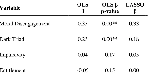
OLS. As previously noted, OLS regression has no hyperparameters. The use of cross-validation is unnecessary with OLS. I simply trained the model on the entire training set using linear modeling (i.e., the lm function) in base R. I then used the trained model to predict CWBs for cases in the test set. Fit statistics for the OLS model are in Table 1. Table 2 presents the beta weights and p-values for each of the MTB scales in the model.
The optimal lambda value from the cross-validated LASSO model using MTB scales was .022. After selecting the lambda value, I then trained a new LASSO model on the entire training set using glmnet. The final training model has the same beta weights as the cross-validated model. In this sense, while it does have a hyperparameter, LASSO is unique due to the inherent connection between its model parameters and its hyperparameter. Specifically, LASSO is a regularization process that should help prevent over-fitting. Finally, I used the trained LASSO model to predict CWBs for cases in the test set. Fit statistics for the LASSO model using MTB scales are in Table 1. Table 2 presents the constrained beta weights from the OLS model using MTB scales. Predictors with coefficients greater than zero are significant by nature of having beta weights greater than zero (i.e. not suppressed). The model does not calculate p-values for the beta weights because the weights themselves are constrained values.
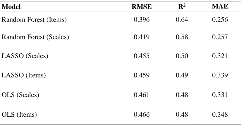
used the trained RF model to predict CWBs for cases in the test set. Model fit indices for the RF model using MTB scales are in Table 1. The RF model using anti-social beliefs/traits scales as predictors had a lower MSE, a lower MAE, and a higher R2 than the OLS and LASSO models using the same methods. Results support Hypothesis 1.
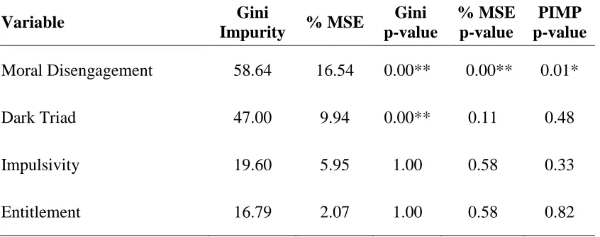
I calculated the RF variable importance metrics on the trained model. The randomForest package provides estimates of the Gini impurity and percent increase to MSE metrics but does not generate p-values (i.e. significance values) for these metrics. I used a permutation approach to generate p-values for these metrics using the rfPermute package (Archer, 2018). This
approach permutes (shuffles) each predictor’s values across observations (participants) a set number of times, creating a set of permuted versions of the original variables. The algorithm then estimates variable importance metrics for each of these permuted variables in order to create a distribution of null importances for each variable. This method then generates probability values (p-values) for observing a variable’s non-permuted importance statistic within the null
Maladaptive Traits/Beliefs Item Level Analysis
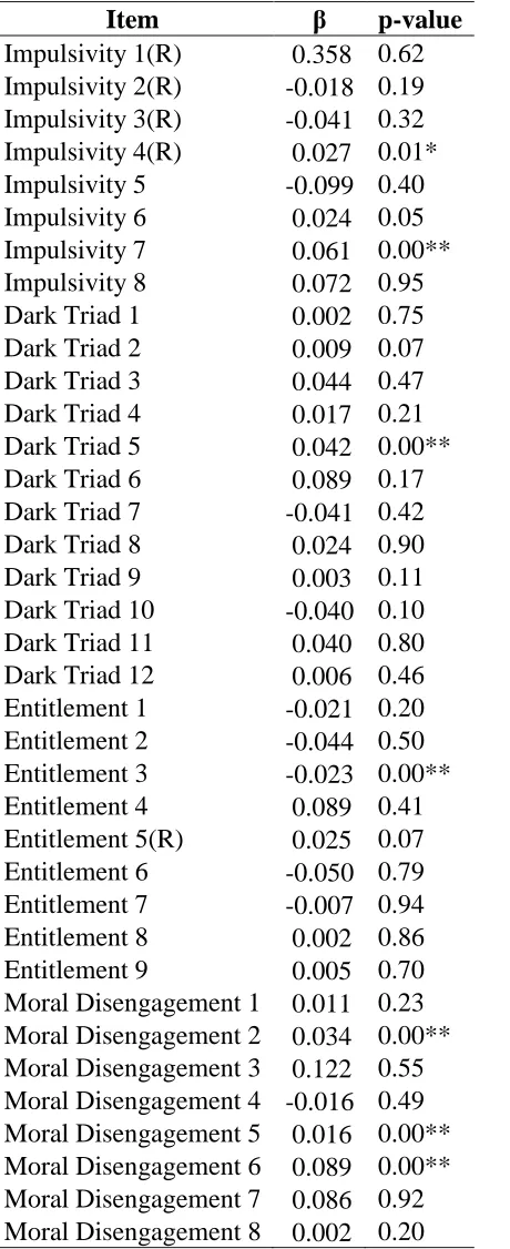
OLS. I trained the OLS model using MTB items as predictors on the entire training set using the lm function in base R. I then used the trained model to predict CWBs for cases in the test set. Model fit results from the OLS regression using MTB items are in Table 1. For
answering research question 1, Table 4 contains linear regression beta weights for each of the MTB items.
LASSO. I used the glmnet package in R to compute results for the LASSO model using MTB items as predictors and again standardized the predictor variables within the glmnet function. I used the caret package to cross-validate the LASSO model, using the same grid search method previously noted, to select the best lambda constraint value, which was .017. After selecting the optimal lambda value, I then trained a new LASSO model on the entire training set using glmnet. Results from LASSO model using MTB items are in Table 1. For answering research question 1, Table 5 contains the LASSO beta weights for each of the MTB items.
Finally, I used the trained RF model to predict CWBs for cases in the test set. Model fit indices for the RF model using all MTB items are in Table 1. The RF model created using MTB items as predictors had a lower RMSE, a lower MAE, and a higher R2 than the OLS and LASSO models created using MTB items. Results support Hypothesis 2a.
Hypothesis 2b stated that the RF model using MTB items as predictors would have higher predictive power than the RF model using MTB scales as predictors. The RF model using MTB items as predictors had a lower RMSE than the RF model using MTB scales, but the two models had roughly equivalent MAE values with a difference of .001. The former model does have a higher R2 value, but this estimate is likely biased when comparing models using different predictor sets. In general, making comparisons between non-nested models that use different predictor sets is generally difficult because both out-of-sample prediction and parsimony are important concepts when comparing models. The purpose for comparing RF models in the current study is to generate a wider sense of how RF models will function using traditional psychology approaches (scale aggregation) compared to item level analysis. It seems that the RF model using all MTB items functioned only marginally better than the RF model using MTB scales as predictors. To assess hypothesis 2b further, I conducted a variable reduction approach on the RF model using MTB items.
using the optimized lambda. RF uses very different variable importance metrics for determining which variables are most important for prediction. Two of the three RF variable importance metrics use permutations to assess the importance of items; the other metric (Gini) assesses the rate at which the RF model uses a variable to make splits.
Importantly, the pragmatic reason for assessing variable importance is so researchers can remove unimportant variables, in this case scale items. Researchers can potentially use these importance metrics to decrease the number of items included in psychological instruments. LASSO performs a kind of variable removal process by constraining beta weights to zero. RF has a different procedure for variable reduction. The RF model using MTB items as predictors has a much greater number of features than the RF model using MTB scales as predictors, so I illustrated the variable reduction approach using the former. Specifically, I used the model training method illustrated by Altmann and colleagues (2010) to remove items with non-significant PIMP variable importance metrics before training a new RF model after the
support for Hypothesis 2b. In addition, these results clearly illustrate the utility of RF models relative to LASSO models for variable importance analysis and item reduction.
Differences in Variable Importance Rankings
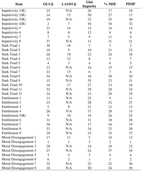
The research question for this study concerned the differences in variable importance ratings across different approaches (models) when the predictors were MTB items. Table 7 presents the MTB items’ variable importance rankings across each of the three models using MTB items as predictors of CWBs. The table shows that item rank ordering across the metrics is similar but does fluctuate across the different metrics. Notably, the two moral disengagement items selected for the final reduced RF model have top rankings across all metrics. This would suggest that the PIMP method is effective in selecting predictors that show consistent significant links to the outcome variable. Furthermore, the PIMP method appears well suited for item level analysis in social science due to its performance in selecting significant items even among highly correlated items.
Discussion
In general, results from this study support the utility of RF models for predicting
important outcomes in social science, and more specifically deviant behavior. Findings from this study support Hindman’s (2015) assertion that ML algorithms can outperform traditional
regression approaches such as OLS (linear regression). Furthermore, this study demonstrates the appropriate steps for conducting RF and provides the computer code (R code) to run the
have use for algorithms and products of computer science. It is likely difficult for social
scientists to implement ML due to lack of concrete examples of ML algorithms applied to social science data and a lack of computer programming knowledge necessary to perform these
analyses. This study helps bridge the gap between two fields by providing an example
application of ML to social science data as well as illustrative and generalizable programming code to perform these techniques. This can aid other social scientists and help them to make use of valuable new analytic resources.
Hypothesis 1 addressed the ability of RF models to outperform traditional linear models when using the typical social science approach of aggregating items into scales. The RF model using MTB scales as predictors explained an additional ten percent of variance over the OLS model using scales as predictors and an additional eight percent of variance over the LASSO model using scales as predictors. This study demonstrates the ability of ML algorithms to outperform traditional regression approaches using the typical predictors of social science data, i.e. psychometric scales.
lowers their predictive power when applied to new data (i.e. test data). The design of RF models reduces the issue of over-fitting, which in turn helps to maintain predictive accuracy when applying these models to new data. Another likely reason the RF models performed better is that there is some degree of non-linearity in the relationship between predictor variables and the target outcome (CWBs). RF models can account for non-linearity in the relationship between predictors and CWBs while OLS and LASSO cannot.
Hypothesis 2b claimed that an RF model would function better when using individual scale items as predictors rather than using the typical approach of aggregating items into scale scores as predictors. While the RF item model did have a lower RMSE than the RF scale model, the two models had roughly equivalent MAEs. The more important finding here, though, is that after variable reduction, the final reduced item RF model used only 6% of the original predictors (i.e., two items) and improved across fit indices compared to the RF model that included all 37 items. Therefore, I contend that researchers should chose the reduced item RF model as the best model for prediction due to its out-of-sample performance and parsimony. This finding greatly supports the utility of RF variable importance metrics and underlines the fact that using RF modeling on social science data has clear pragmatic applications.
The research question for this study addressed the difference in variable importance metrics for MTB items across algorithms. The RF model provides a wider range of item importance indicators, which researchers can use to decide which items to remove while
node, relative to other items under consideration within the model. Second, the permuted percent increase in MSE metric shuffles a predictor variable’s values across observations and then runs the RF model using the permuted (shuffled) version of the variable. The calculation then compares the MSE of the RF model using the un-permuted variable to that of the model using the permuted variable. The difference indicates the loss in accuracy the model suffers because of using the permuted version of a variable. In this sense, an item’s importance is equivalent to its impact on the model’s fit indices. Finally, the Altman (2010) permutation importance (PIMP) is the most computationally heavy index and appears to be the most stringent of the item
importance indices. This method permutes the outcome variable rather than the predictor
variables, thus preserving the relationships between predictors. Using multiple permutations, this method creates a null distribution of variable importances, which the model uses to generate p-values for each variable’s importance (Gini) metric. For this method, a variable’s importance represents its ability to predict the target outcome while considering its relationship to other predictors in the model. While it is common for researchers to refer to ML algorithms as black box phenomena (Card, 2017), RF models actually provide more information about the
functionality of predictors (features) than traditional regression approaches. A wider range of variable importance indicators provides researchers with more information to leverage when deciding which items to remove. This can aid researchers in reducing the number of item in psychometric instruments while still maintaining confidence that the remaining items will retain previous levels of predictive capability.
To illustrate the value of RF variable importance metrics, I conducted a variable
variable RF model. This reduced RF model had the best predictive power compared to all other models and used only two of the original thirty-seven scale items. This magnitude of variable reduction displayed in the current study is promising; researchers have not previously
demonstrated such stark results using OLS approaches. This final reduced model represents the best fitting model and the most parsimonious of all study models. This study has fully
demonstrated the utility of RF using the current data set.
Another major contribution of this study is the R code that I produced and attached to this document. Without doubt, ML topics have gained popularity in social science, but social
scientists may encounter difficulty when attempting to apply ML to prediction efforts in their respective fields. The vast majority of ML research exists in journals well outside of social science. Furthermore, researchers with limited coding experience will certainly encounter difficulty when attempting to set up ML algorithms. This study, and the annotated R code, documents the process of implementing LASSO and RF regression from the perspective of a social science researcher. Furthermore, the R code is generalizable (i.e. soft-coded), meaning researchers can use the code for their own studies by following the short instructions at the beginning of the R document (Appendix G). For example, a personality researcher could repurpose the prediction analyses from this study to use on a data set that includes the Big-Five personality index as indicators and any continuous outcome of interest. No alteration to the fundamental analysis code is necessary.
relevant predictor items greatly. Perhaps even more important to I/O psychologists, forensic psychologists, and criminologists is the nature of the two remaining items. Both items with significant variable importance (PIMP) belonged to the moral disengagement scale. The first item, moral disengagement six, reads “Taking personal credit for ideas that were not your own is no big deal.” The second item, moral disengagement two, reads “Taking something without the owner’s permission is okay as long as you’re just borrowing it.” The content of these two items converges around the notion of wrongfully taking something of value, either social credit or physical objects. It seems logical that these two items would predict workplace deviance well. Limitations
Researchers should take some caution when generalizing findings from the current study to new scenarios. The context of the target behavior is likely important. The RF item reduction process created a narrow predictor set that is specifically suited to predict CWBs. That is, had the target outcome been criminal behavior or arrest rates, different MTB items may have performed better. This is an obvious topic for future research, and the code provided in this document would make the application to new data sets straightforward. Additionally, the randomForest package will automatically adapt for categorical or continuous outcomes, such that the provided R code can generalize to categorical outcomes with only few alterations to the code generating fit statistics. Researchers can use the provided code to generalize the analyses in this study and produce results that are relevant to different target behaviors.
addition, responding to only two predictor items would almost certainly influence the way that participants respond to the survey items. For example, survey respondents may be more likely to alter or distort their responses if they know that only two items will represent their characteristics on a survey. In an applied setting, such as employee selection, using only two indicator items may influence survey respondents’ perceptions of face validity or their perceptions of justness regarding the selection instrument. In other words, there may be many unforeseen consequences of such a drastic reduction in survey length. Instead, researchers should consider these results as an opportunity to search for new relevant predictors. Future studies on CWBs should examine new measures in addition to the measures/items that were significant in the present study.
The RF item reduction process outlined in this study is not a replacement for
Concluding Remarks
Interest in ML topics is on the rise in social sciences, with the Society for Industrial and Organizational Psychology (SIOP) preparing to host its 2nd annual ML competition. Nonetheless, social scientists may encounter roadblocks when trying to apply ML to their respective fields. One roadblock is the lack of information on ML within social science literature, forcing
References
Altmann, A., Tolosi, L., Sander, O., & Lengauer, T. (2010). Permutation importance: A corrected feature importance measure. Bioinformatics, 26, 1340–1347.
Andrews, J. S. (2018). A Tale of Two Constructs: Defining Integrity and Corruption, Clarifying Their Factor Structures and Examining Their Association with Organizational
Citizenship and Counterproductive Work Behaviors. Unpublished Master’s Thesis. North Carolina State University, Raleigh, N.C.
Andrews, J. S., Thompson, I.B., & Williams, L. J. (2016). Examining the relationship between moral cognition and counterproductive work behaviors. Poster presented at the annual meeting for the Society for Industrial and Organizational Psychology, Anaheim, CA. Archer, E. (2018). rfPermute: Estimate permutation p-values for random forest importance. R
package version 2.1.6. https://CRAN.R-project.org/package=rfPermute.
Bandura, A. (1990) Mechanisms of moral disengagement, in: W. REICH (Ed.), Origins of
Terrorism: psychologies, ideologies, theologies, states of mind, pp. 161–191.
Bandura, A. (2002). Selective Moral Disengagement in the Exercise of Moral Agency. Journal
of Moral Education, 31, 101−119.
Benda, B. B. (2003). A Test of Three Competing Theoretical Models of Delinquency Using Structural Equation Modeling, Journal of Social Service Research, 29:2, 55–91. Breiman, L. (2001). Random forests. Machine Learning, 45, 5–32.
Breiman, L. Friedman, J. H., Olshen, R. A. & Stone, C. J. (1984). Classification and regression
trees. Chapman and Hall: London, U.K.
Campbell, W. K., Bonacci, A. M., Shelton, J., Exline, J. J., & Bushman, B. J. (2004).
measure. Journal of Personality Assessment, 83, 24–45.
Card, D. (2017, July). The black box metaphor in machine learning. Towards Data Science. Retrieved from: https://towardsdatascience.com/the-black-box-metaphor-in-machine-learning-4e57a3a1d2b0.
Celik, E. (2015). Vita: Variable importance testing approaches. R package version 1.0.0. https://CRAN.R-project.org/package=vita.
Cohen, T. R., Panter, A. T., Turna, N., Morse, L. & Kim, Y. (2014). Moral Character in the Workplace. Journal of Personality and Social Psychology, 107, 943−963.
Friedman, J., Hastie, T., & Tibshirani, R. (2010). Regularization paths for generalized linear models via coordinate descent. Journal of Statistical Software, 1, 1−13.
Hindman, M. (2015). Building Better Models. The Annals of the American Academy, 659, 48– 62.
Jonason, P. K. & Webster, G. D. (2010). The dirty dozen: A concise measure of the dark triad.
Psychological Assessment, 22, 420–432.
Knight, K., Garner, B. R., Simpson, D. D., Morey, J., & Flynn, P. M. (2006). An assessment for criminal thinking. Crime and Delinquency, 52, 159−177.
Kuhn, M. (2008). Building predictive models in R using the caret package. Journal of Statistical
Software, 28, 1–26.
Leeman, R. F., & Potenza, M. N. (2012). Similarities and differences between pathological gambling and substance use disorders: A focus on impulsivity and compulsivity.
Psychopharmacology, 219, 469–490.
Loomis v. Wisconsin, 137 S.Ct. 2290 (June, 2017).
Mandell. W. (2006). Predicting institutional adjustment with the psychological inventory of criminal thinking styles and the psychopathology checklist: Screening version
(Unpublished doctoral dissertation). Philadelphia College of Osteopathic Medicine
Department of Psychology, Philadelphia, P.A.
Moan, I. S., Nordstrom, T., & Storvoll, E. E. (2013). Alcohol use and drunk driving: The
modifying effect of impulsivity. Journal of Studies on Alcohol and Drugs, 74, 114–119. Moore, C., Detert, J. R., Trevino, L. K., Baker, V. L., & Mayer, D. M. (2012). Why employees
do bad things: Moral disengagement and unethical organizational behavior. Personnel
Psychology, 65, 1–48.
Morean, M. E., DeMartini, K. S., Leeman, R. F., Pearlson, G. D., Anticevic, A., Krishnan-Sarin, S., Krystal, J. H., & O’malley, S. S. (2012). Psychometrically improved, abbreviated, version of three classic measures of impulsivity and self-control. Psychological
Assessment, 26, 1003–1020.
Nawara, S. (2019). Avoiding data leakage in machine learning. Conlan Scientific. Retrieved from: https://conlanscientific.com/posts/category/blog/post/avoiding-data-leakage-machine-learning/
O’Boyle, E. H., Forsyth, D. R., Banks, G. C., & McDaniel, M. A. (2012). A meta-analysis of the dark triad and work behavior: A social exchange perspective. Journal of Applied
Psychology, 97, 557–579.
Patton, J. H., Stanford, M.S., & Barratt, E.S. (1995). Factor structure of the Barratt impulsiveness scale. Journal of Clinical Psychology, 51, 768–774.
Probst, P. & Boulesteix, A. L. (2017). To tune or not to tune the number of trees in random forest?. Journal of Machine Learning Research, 18, 1–20.
R Core Team (2018). R: A language and environment for statistical computing. R Foundation for
Statistical Computing, Vienna, Austria. URL http://www.R-project.org/.
Ragatz, L. L., Fremouw, W., & Baker, E. (2012). The psychological profile of white-collar offenders: Demographics, criminal thinking, psychopathic traits, and psychopathology.
Criminal Justice and Behavior, 39, 978–997.
Sauer, S., Lemke, J., Zinn, W., Buettner, R., & Kohls, N. (2015). Mindful in a random forest: Assessing the validity of mindfulness items using random forest methods. Personality
and Individual Differences, 81, 117–123.
Scherer, K. T., Baysinger, M., Zolynsky, D. & LeBreton, J. M. (2013). Predicting
counterproductive work behaviors with sub-clinical psychopathy: Beyond the five factor model of personality. Personality and Individual Differences, 55, 300–305.
Schmidt, F. L., & Hunter, J. E. (1998). The validity and utility of selection methods in personnel psychology: Practical and theoretical implications of 85 years of research findings.
Psychological Bulletin, 14, 262–274.
Spector, P. E. Fox, S., Penney, L. M., Bruursema, K., Goh, A., & Kessler, S. (2006). The dimensionality of counterproductivity: Are all counterproductive behaviors created equal? Journal of Vocational Behavior, 68, 446–460.
Taagepera, R. (2008). Making Social Sciences More Scientific: The Need For Predictive Models. Oxford University Press, Great Clarendon Street, Oxford.
Tibshirani, R. (1996). Regression shrinkage and selection via the lasso. Journal of the Royal
Statistical Society, 58, 276–288.
Van Iddekinge, C. H., Roth, P. L., Raymark, P. H, & Odle-Dusseau, H. N. (2012). The Criterion-Related Validity of Integrity Tests: An Updated Meta-Analysis. Journal of
Applied Psychology, 97, 499–530.
Van Zyl, C.J.J., & De Bruin, G.P.(2018) Predicting counterproductive behaviors with narrow personality traits: A nuanced examination using quantile regression. Personality and
Individual Differences, 131, 45–40.
Wright, M.N. & Zeigler, A. (2017). A fast implementation of random forests for high dimensional data in {C++} and {R}. Journal of Statistical Software, 77, 1–17.
Table 1
Fit Statistics for OLS, LASSO, and RF Models Using Maladaptive Traits/Beliefs Scales and Items to Predict CWBs, (n=99).
Note. CWBs = Counterproductive Work Behavior.
Model RMSE R2 MAE
Random Forest (Items) 0.396 0.64 0.256
Random Forest (Scales) 0.419 0.58 0.257
LASSO (Scales) 0.455 0.50 0.321
LASSO (Items) 0.459 0.49 0.339
OLS (Scales) 0.461 0.48 0.331
Table 2
Beta weights from Linear and LASSO Regression Models Using Anti-Social Beliefs/Traits Scales to Predict CWBs, (n=402).
Note. *p < .05, **p < .01, CWBs = Counterproductive Work Behaviors
Variable OLS β OLS β
p-value
LASSO β
Moral Disengagement 0.35 0.00** 0.33
Dark Triad 0.23 0.00** 0.18
Impulsivity 0.04 0.17 0.05
Table 3
Variable Importance Metrics from Random Forest Model Using Anti-Social Beliefs/Traits Scales to Predict CWBs, (n=402).
Note. *p < .05, **p < .01, CWBs = Counterproductive Work Behaviors.
Variable Gini
Impurity % MSE
Gini p-value
% MSE p-value
PIMP p-value Moral Disengagement 58.64 16.54 0.00** 0.00** 0.01*
Dark Triad 47.00 9.94 0.00** 0.11 0.48
Impulsivity 19.60 5.95 1.00 0.58 0.33
Table 4
Beta weights from Linear Regression Model Using Anti-Social Beliefs/Traits Items to Predict CWBs, (n=402).
Note. *p < .05, **p < .01, CWBs= Counterproductive Work Behaviors.
Item β p-value
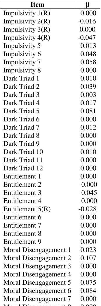
Table 5
Beta weights from LASSO Regression Model Using Anti-Social Beliefs/Traits Items to Predict CWBs, (n=402).
Note. CWBs= Counterproductive Work Behaviors.
Item β
Impulsivity 1(R) 0.000 Impulsivity 2(R) -0.016 Impulsivity 3(R) 0.000 Impulsivity 4(R) -0.047
Impulsivity 5 0.013
Impulsivity 6 0.048
Impulsivity 7 0.058
Impulsivity 8 0.000
Dark Triad 1 0.010
Dark Triad 2 0.039
Dark Triad 3 0.003
Dark Triad 4 0.017
Dark Triad 5 0.081
Dark Triad 6 0.000
Dark Triad 7 0.012
Dark Triad 8 0.000
Dark Triad 9 0.000
Dark Triad 10 0.010
Dark Triad 11 0.000
Dark Triad 12 0.000
Entitlement 1 0.000
Entitlement 2 0.000 Entitlement 3 0.045 Entitlement 4 0.000 Entitlement 5(R) -0.028
Entitlement 6 0.000
Entitlement 7 0.000
Entitlement 8 0.000
Entitlement 9 0.000
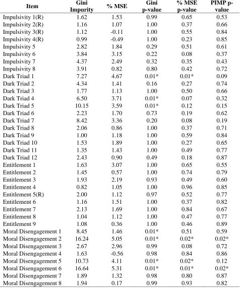
Table 6
Variable Importance Metrics from Random Forest Model Using Anti-Social Beliefs/Traits Items to Predict CWBs, (n=402).
Note. *p < .05, **p < .01, P-values for % increase in MSE and Gini impurity are the scaled
p-values from the rfPermute package in R. CWBs = Counterproductive Work Behaviors.
Item Gini
Impurity % MSE
Gini p-value % MSE p-value PIMP p-value
Impulsivity 1(R) 1.62 1.53 0.99 0.65 0.53
Impulsivity 2(R) 1.16 1.07 1.00 0.37 0.66
Impulsivity 3(R) 1.12 -0.11 1.00 0.55 0.84
Impulsivity 4(R) 0.99 -0.49 1.00 0.23 0.85
Impulsivity 5 2.82 1.84 0.29 0.51 0.61
Impulsivity 6 3.84 3.15 0.22 0.08 0.37
Impulsivity 7 4.37 2.49 0.32 0.35 0.43
Impulsivity 8 3.91 0.82 0.80 0.42 0.72
Dark Triad 1 7.27 4.67 0.01* 0.01* 0.09
Dark Triad 2 4.34 1.41 0.16 0.27 0.74
Dark Triad 3 1.77 1.13 1.00 0.50 0.66
Dark Triad 4 6.50 3.71 0.01* 0.07 0.32
Dark Triad 5 10.15 3.59 0.01* 0.12 0.15
Dark Triad 6 2.23 1.70 0.73 0.19 0.62
Dark Triad 7 8.42 3.36 0.20 0.08 0.19
Dark Triad 8 2.06 0.86 1.00 0.37 0.71
Dark Triad 9 1.00 1.18 1.00 0.59 0.84
Dark Triad 10 1.53 1.89 1.00 0.27 0.65
Dark Triad 11 1.35 1.43 1.00 0.49 0.77
Dark Triad 12 2.43 0.90 0.49 0.18 0.87
Entitlement 1 1.63 3.07 1.00 0.65 0.55
Entitlement 2 1.45 0.57 1.00 0.74 0.79
Entitlement 3 1.93 2.19 0.93 0.49 0.60
Entitlement 4 0.82 1.05 1.00 0.96 0.85
Entitlement 5(R) 2.00 1.12 0.97 0.52 0.77
Entitlement 6 1.16 1.51 1.00 0.37 0.82
Entitlement 7 2.13 1.69 1.00 0.84 0.67
Entitlement 8 1.04 1.12 1.00 0.47 0.77
Entitlement 9 1.08 0.36 1.00 0.46 0.89
Moral Disengagement 1 8.45 1.46 0.01* 0.51 0.59
Moral Disengagement 2 16.24 5.05 0.01* 0.02* 0.02*
Moral Disengagement 3 2.67 2.96 0.99 0.08 0.72
Moral Disengagement 4 1.63 -0.56 0.98 0.84 0.86
Moral Disengagement 5 10.73 4.11 0.01* 0.02* 0.12
Moral Disengagement 6 16.64 5.31 0.01* 0.01* 0.02*
Moral Disengagement 7 1.89 1.32 0.98 0.80 0.87
Table 7
OLS, LASSO, and RF Item Importance Ranks for Maladaptive Traits and Beliefs Items Across Variable Importance Metrics.
Note. N/A under LASSO results is for items with beta weights reduced to zero.
Item OLS β LASSO β Gini
Impurity % MSE PIMP
Impulsivity 1(R) 25 N/A 26 17 10
Impulsivity 2(R) 14 13 30 27 17
Impulsivity 3(R) 19 N/A 32 35 30
Impulsivity 4(R) 2 7 36 36 32
Impulsivity 5 21 14 13 14 14
Impulsivity 6 8 6 12 8 8
Impulsivity 7 7 5 9 11 9
Impulsivity 8 37 N/A 11 31 21
Dark Triad 1 30 16 7 3 3
Dark Triad 2 10 9 10 21 23
Dark Triad 3 26 18 23 24 18
Dark Triad 4 12 12 8 5 7
Dark Triad 5 4 3 4 6 5
Dark Triad 6 13 N/A 16 15 15
Dark Triad 7 22 15 6 7 6
Dark Triad 8 34 N/A 18 30 20
Dark Triad 9 15 N/A 35 23 31
Dark Triad 10 16 17 27 13 16
Dark Triad 11 32 N/A 29 20 24
Dark Triad 12 24 N/A 15 29 35
Entitlement 1 11 N/A 25 9 11
Entitlement 2 23 N/A 28 32 27
Entitlement 3 5 8 21 12 13
Entitlement 4 20 N/A 37 28 33
Entitlement 5(R) 9 10 19 26 25
Entitlement 6 31 N/A 31 18 28
Entitlement 7 36 N/A 17 16 19
Entitlement 8 33 N/A 34 25 26
Entitlement 9 29 N/A 33 33 37
Moral Disengagement 1 17 11 5 19 12
Moral Disengagement 2 1 1 2 2 1
Moral Disengagement 3 28 N/A 14 10 22
Moral Disengagement 4 27 N/A 24 37 34
Moral Disengagement 5 3 4 3 4 4
Moral Disengagement 6 6 2 1 1 2
Moral Disengagement 7 35 N/A 22 22 36
Appendix A
Counterproductive Work Behavior Scale items Spector, Fox, Penney, Bruursema, Goh, and Kessler (2006)
Prompt: “How often have you done each of the following things on your job(s) within the past year?”
Scale Anchors: 1 (Never), 2 (Once or twice), 3 (Once or twice per month), 4 (Once or twice per week), 5 (Everyday).
1. Purposely wasted your employer’s materials/supplies 2. Purposely damaged a piece of equipment or property 3. Purposely dirtied or littered your place of work 4. Came to work late without permission
5. Stayed home from work and said you were sick when you were not 6. Taken a longer break than you were allowed to take
7. Left work earlier than you were allowed to 8. Purposely did your work incorrectly
9. Purposely worked slowly when things needed to get done 10.Purposely failed to follow instructions
11.Stolen something belonging to your employer 12.Took supplies or tools home without permission 13.Put in to be paid for more hours than you worked 14.Took money from your employer without permission 15.Stole something belonging to someone at work
16.Told people outside the job what a lousy place you work for 17.Started or continued a damaging or harmful rumor at work 18.Been nasty or rude to a client or customer
19.Insulted someone about their job performance 20.Made fun of someone’s personal life
21.Ignored someone at work
22.Blamed someone at work for error you made 23.Started an argument with someone at work 24.Verbally abused someone at work
25.Made an obscene gesture (the Finger) to someone at work 26.Threatened someone at work with violence
27.Threatened someone at work, but not physically
28.Said something obscene to someone at work to make them feel bad 29.Did something to make someone at work look bad
30.Played a mean prank to embarrass someone at work
31.Looked at someone at work’s private mail/property without permission 32.Hit or pushed someone at work
Appendix B
The Dirty Dozen (Dark Triad) Jonason & Webster (2010)
Prompt: “Please indicate how much you agree with the following statements.”
Anchors: 1 (Strongly Disagree), 2 (Disagree), 3 (Neither Disagree nor Agree), 4 (Agree), 5 (Strongly Agree).
1. I tend to manipulate others to get my way. 2. I have used deceit or lied to get my way. 3. I have used flattery to get my way.
4. I tend to exploit others towards my own end. 5. I tend to lack remorse.
6. I tend to be unconcerned with the morality of my actions. 7. I tend to be callous or insensitive.
8. I tend to be cynical.
9. I tend to want others to admire me.
10.I tend to want others to pay attention to me. 11.I tend to seek prestige or status.
Appendix C
Shortened Barratt Impulsiveness Scale (BIS) Items
Morean, DeMartini, Leeman, Pearlson, Anticevic, Krishnan, Krystal, & O’Malley (2014) Prompt: “Please indicate how much you agree with the following statements.”
Anchors: 1 (Strongly Disagree), 2 (Disagree), 3 (Neither Disagree nor Agree), 4 (Agree), 5 (Strongly Agree).
1. I plan tasks carefully. (R) 2. I am self-controlled. (R) 3. I concentrate easily. (R) 4. I am a carful thinker. (R) 5. I do things without thinking 6. I don’t pay attention
Appendix D Psychological Entitlement
Campbell, Bonacci, Shelton, Exline, & Bushman (2004) Prompt: “Please indicate how much you agree with the following statements.”
Anchors: 1 (Strongly Disagree), 2 (Disagree), 3 (Neither Disagree nor Agree), 4 (Agree), 5 (Strongly Agree).
1. I honestly feel I’m just more deserving than others. 2. Great things should come to me.
3. If I were on the titanic, I would deserve to be on the first lifeboat! 4. I demand the best because I’m worth it.
5. I don’t necessarily deserve special treatment. (R) 6. I deserve more things in my life.
7. People like me deserve an extra break now and then. 8. Things should go my way.
Appendix E Moral Disengagement
Moore, Detert, Trevino, Baker, & Mayer (2012) Prompt: “Please indicate how much you agree with the following statements.”
Anchors: 1 (Strongly Disagree), 2 (Disagree), 3 (Neither Disagree nor Agree), 4 (Agree), 5 (Strongly Agree).
1. It is okay to spread rumors to defend those you care about.
2. Taking something without the owner’s permission is okay as long as you’re just borrowing it.
3. Considering the ways people grossly misrepresent themselves, it’s hardly a sin to inflate your own credentials a bit.
4. People shouldn’t be held accountable for doing questionable things when they were just doing what an authority figure told them to do.
5. People can’t be blamed for doing things that are technically wrong when all their friends are doing it too.
6. Taking personal credit for ideas that were not your own is no big deal.
Appendix F Demographic Questions Prompt: “Please respond to the following demographic questions.”
1. What is your age in years?
2. What is your biological sex? (Male/Female)
3. What gender do you identify with? (Male/Female/Neither) 4. What country do you reside in?
5. How many hours do you typically work in a week?
6. Are you currently employed part-time (28 hours per week or less) or full-time (29+ hours per week)?
7. Have you worked full-time for at least one year? (Yes/No) 8. Do you have more than one employer? (Yes/No)
a. If Yes: How many different employers do you have? 9. How long have you been with your current employer?
a. If yes to question 8: How long have you been with your current employers? (Spaces provided for multiple entries)
10.Which of the following occupations bests describes your work? a. Management Occupations
b. Business and Financial Operations Occupations c. Computer and Mathematical Occupations d. Architecture and Engineering Occupations e. Life, Physical, and Social Science Occupations f. Community and Social Service Occupations g. Legal Occupations
h. Education, Training, and Library Occupations
i. Arts, Design, Entertainment, Sports, and Media Occupations j. Healthcare Practitioners and Technical Occupations
k. Healthcare Support Occupations l. Protective Service Occupations
m. Food Preparation and Serving Related Occupations
n. Building and Grounds Cleaning and Maintenance Occupations o. Personal Care and Service Occupations
p. Sales and Related Occupations
q. Office and Administrative Support Occupations r. Farming, Fishing, and Forestry Occupations s. Construction and Extraction Occupations
t. Installation, Maintenance, and Repair Occupations u. Production Occupations