The Stability and Control of an Aircraft with an Adaptive Wing

(1)

ABSTRACT

VOSBURG, VICTOR JAY. The Stability and Control of an Aircraft with an Adaptive Wing. (Under the direction of Dr. Ashok Gopalarathnam.)

(2)

The Stability and Control of an Aircraft with an

Adaptive wing

by

Victor J. Vosburg

A thesis submitted to the Graduate Faculty of North Carolina State University

in partial fulfillment of the requirements for the Degree of

Master of Science

Aerospace Engineering

Raleigh, NC 2004

APPROVED BY:

Dr. Ashok Gopalarathnam Advisory Committee Chairman

(3)

To all my friends and family

(4)

BIOGRAPHY

Victor Jay Vosburg was born in Wilmington, NC on May 12, 1979, to Robert and Barbara Vosburg. He was raised in Ruffin, NC with his younger brother Ross. He graduated from Rockingham High School in 1997 and started his studies at North Carolina State University. He received a BS in Aerospace Engineering on May 15, 2002 with a Minor in Business Management.

(5)

ACKNOWLEDGEMENTS

This thesis would not have been possible without the guidance and assistance of my advisor, Dr. Ashok Gopalarathnam. His dedication, support, high expecta-tions of his students have provided me with the ability to successfully complete my research.

I would also like to thank Dr. Charles Hall and Dr. Arkady Kheyfets for agree-ing to be on my advisory committee. I am privileged to have taken classes with both of them and appreciate the knowledge that they have provided.

I would like to thank The Clair Hunnicutt Scholarship for its support in pro-viding my education.

I would like to acknowledge Unmanned Dynamics for the educational use of the AeroSim blockset. This software greatly helped me in the pursuit of my research goals.

(6)

List of Tables

(9)

List of Figures

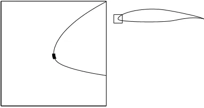
1.1 (a) Geometry of airfoil with a TE flap, and typical locations of the four pressure sensors referred to in Section 1.1.2,and (b) drag polars showing effectiveness of TE flap in adapting the drag polar to suit

a wide range of lift coefficients. . . 2

1.2 Variation of the stagnation-point location with airfoil lift coefficient for flap deflections of₋10, ₋5, 0, 5, and 10 degrees. . . 3

1.3 Geometry of the airfoil with inset showing desired range for stagnation-point location. . . 3

1.4 ∆C0 p vs. Cl “calibration” curves for different flap angles showing desirable range of ∆C0 p that results in low drag. . . 4

1.5 Comparison of the drag polars and lift and pitching-moment curves for the example NLF airfoil with automated cruise flaps and with-out flaps. . . 5

2.1 Planview showing the right-side geometry of the wing and tail for the Aerosonde UAV used in this paper. . . 9

2.2 Demonstration of the drag polar shift due to a change in the flap angle for the AeroSim method (Eq. 2.7). . . 12

2.3 Demonstration of the drag drag polar shift due to a change in the flap angle for the new method (Eq. 2.8) . . . 14

3.1 CM,cg vs. α comparison for fixed elevator for two flap settings. . . 17

3.2 AirfoilCl vs.αcurve for two flap angles to illustrate flap-controller behavior. . . 19

4.1 Nonlinear open-loop model for studying the step response to the flap angle. . . 25

4.2 Linear open-loop model for studying the step response to the flap angle. . . 25

4.3 Comparison of Linear, Nonlinear, and Static results.(a) Flap An-gle,(b) Velocity response, and (c) Alpha response. . . 26

4.4 Model for closed loop simulation. . . 27

4.5 Flap and elevator controllers with no coupling. . . 29

4.6 Exploded block diagram of the flap controller. . . 30

(10)

4.8 Comparison of aircraft response with and without flap-elevator cou-pling: (a) velocity, (b) flap angle, and (c) elevator angle . . . 32 4.9 Response of aircraft to step change in the desired velocity for several

flap-actuation frequencies: (a) velocity (b) flap angle (c) altitude (d)throttle. Both (e) and (f) are the zoomed in views of the velocity and throttle after the change in desired velocity. . . 33 4.10 Demonstration of drag benefits of the adaptive aircraft during

sim-ulation. The figures are: (a) flap deflection, (b) Coefficient of Drag (CD), (c) throttle setting,(d) fuel consumption, (e) velocity, and (f)

(11)

Nomenclature

AR aspect ratio b wing span c chord length

Cd airfoil drag coefficient

CD0 aircraft min drag coefficient CL aircraft lift coefficient

Cl airfoil lift coefficient

CL0 aircraft lift coefficient for min drag CM aircraft pitching moment coefficient

Cm airfoil pitching moment coefficient

Cp airfoil pressure coefficient

∆C0

p pressure coefficient Eq. 1.1

i incidence

K 3D correction factor

lt tail moment arm measured to ac of the wing

M Mach number mac mean chord length p pressure

Re Reynolds number

S area

(12)

Vh horizontal tail volume ratio referenced to ac

Vm max velocity

x x-coordinate α angle of attack

δ control surface deflection

downwash

η efficiency factor for tail φ bank angle

θf angular location of flap hinge in radians

Subscripts

ac aerodynamic center a aileron

cg center of gravity e elevator

f flap f lapped flapped f us fuselage

ideal ideal condition from thin airfoil theory l location near mid chord on the lower surface ll location near leading edge on the lower surface n neutral point

p propulsion system ref reference, wing r rudder

t tail

u location near mid chord on the upper surface uu location near leading edge on the upper surface

(13)

Chapter 1 Introduction

A well-known means of adapting an airfoil to achieve low drag over a large lift range is by means of a trailing-edge cruise flap. Recent research has provided a means of automating the cruise flap to achieve the benefits of improved aircraft performance without an increase in pilot workload. In this research, the stability and control aspects of an aircraft with such an adaptive wing are studied.

1.1 Background

1.1.1 Airfoil Adaptation Using a Camber-Changing TE

Flap

Adaptive wings are receiving increasing attention for their potential to reduce aircraft drag over a large speed range.1, 2 _{One of the elementary forms of wing}

(14)

condi-Flap = −5 deg Flap = 0 deg Flap = 5 deg

plu pu

pll pl

−0.5 0 0.5 1 1.5 2 −5 −4 −3 −2 −1 0 1

−10ο flap −5ο flap 0ο flap 5ο flap 10ο flap

∆C p ′ C l (a) (b)

0 0.005 0.01 0.015 0.02 0

0.5 1 1.5

10 deg flap 5 deg flap 0 deg flap −5 deg flap −10 deg flap LDR upper corner LDR lower corner

C

d

C

l

(b)

−30 −2 −1 0 1 0.5 1 1.5 ∆C p ′ C l (c) desirable range of ∆C

p

′_{for low drag}

Figure 1.1: (a) Geometry of airfoil with a TE flap, and typical locations of the four pressure sensors referred to in Section 1.1.2,and (b) drag polars showing effectiveness of TE flap in adapting the drag polar to suit a wide range of lift coefficients.

tion.3 _{Figure 1.1(b), from Refs. 4 and 5, shows how a cruise flap results in an}

effectively larger drag bucket when compared to the zero-degree flap setting. The results were obtained using the XFOIL code,6 _{and were validated using}

experi-mental data in Ref. 4. On sailplanes, the flap is set to the correct angle by the pilot for any given airspeed using some form of a lookup table and the reading of the airspeed indicator. While this increased pilot workload is tolerated in the world of competition sailplanes, this increased workload is believed to be an im-portant reason why cruise flaps have not become popular on general aviation and other commercial aircraft.

1.1.2 Recent Auto-Adaptive Airfoil Research at NCSU

With an ultimate objective of bringing the performance benefits of cruise flaps to current-day piloted aircraft and enabling their use on uninhabited aerial vehicles (UAVs) and future autonomous aircraft, recent NCSU research by McAvoy and Gopalarathnam sought to automate the cruise flap based on the flow conditions sensed at the airfoil. The results of the concept development, estimated benefits,4, 5

and wind-tunnel closed-loop demonstration4 _{are presented in this subsection in an}

(15)

−0.5 0 0.5 1 1.5 1.02

1.03 1.04 1.05 1.06 1.07 1.08 1.09

C

l

s/c

−10 deg flap −5 deg flap 0 deg flap 5 deg flap 10 deg flap

lower corner upper corner

s/c

Figure 1.2: Variation of the stagnation-point location with airfoil lift coefficient for flap deflections of ₋10, ₋5, 0, 5, and 10 degrees.

Figure 1.3: Geometry of the airfoil with inset showing desired range for stagnation-point location.

described in this thesis.

It has been known for some time that a cruise flap works by bringing the stagnation point to a small desirable region near the leading edge, thus resulting in favorable velocity gradients on both the upper and lower surfaces of the airfoil.3, 7

(16)

Flap = −5 deg Flap = 0 deg Flap = 5 deg

plu

pu

pll pl

−0.5 0 0.5 1 1.5 2

−5 −4 −3 −2 −1 0 1

−10ο flap

−5ο flap

0ο flap

5ο flap

10ο flap

∆C p ′ C l (a) (b)

0 0.005 0.01 0.015 0.02

0 0.5 1 1.5

10 deg flap 5 deg flap 0 deg flap −5 deg flap −10 deg flap LDR upper corner LDR lower corner

C

d

C

l

(b)

−30 −2 −1 0 1

0.5 1 1.5 ∆C p ′ C l desirable range

of ∆C

p

′_{for low drag}

Figure 1.4: ∆C0

p vs. Cl “calibration” curves for different flap angles showing

desirable range of ∆C0

p that results in low drag.

quantified in Refs. 4 and 5. As a result of this behavior, the boundary layers on both the upper and lower surfaces experience favorable pressure gradients, thus promoting laminar flow (where transition is governed by the growth of T-S waves) over a wide range of lift coefficients.

For automating the cruise flap, a pressure-based sensing approach was devel-oped by hypothesizing that if the stagnation point is indeed located within a small region when the flap is set to the optimum angle, then the pressure distribution in the vicinity of the leading edge should also be quite similar. A systematic computational study with XFOIL was used to develop a scheme where pressure measurement at just four locations on the airfoil surface could be used to sense the airfoil Cl and also set the flap to the correct angle. The four pressure

mea-surements are used to define a non-dimensional ∆C0

p that is shown in Eq. 1.1.

Figure 1.1(a) shows the typical locations of the four pressure ports on the airfoil, and Fig. 1.1(c) shows the variation of ∆C0

p with Cl for various flap settings. Two

important observations can be made, both of which were verified4, 5 _using

(17)

0 0.01 0.02 0 0.5 1.0 1.5 C d C l

No flap deflection Automated cruise flap

= 2×106 Re C

l 1/2

−5 0 5 10 0

0.5 1.0 1.5

α (deg) C l 0 −0.1 −0.2 0.1 C m

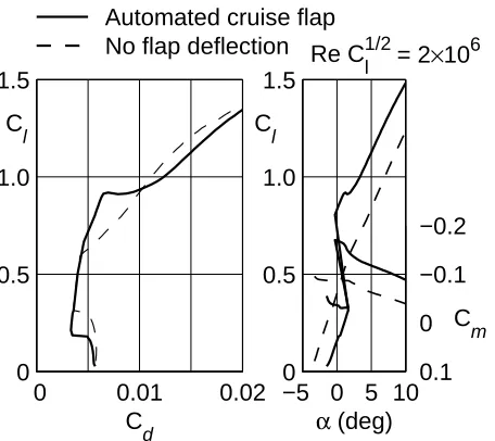
Figure 1.5: Comparison of the drag polars and lift and pitching-moment curves for the example NLF airfoil with automated cruise flaps and without flaps.

1. For any given Cl if the flap angle is set to maintain the ∆Cp0 within a

desirable range, then the airfoil operates close to the minimum drag for that condition.

2. The ∆C0

p curves in Fig. 1.1(c) can be used as “calibration curves” so that if

the flap angle and the ∆C0

p are known, then the airfoilClcan be determined.

∆C0

p =

plu−pll

|pu −pl|

= Cplu−Cpll

|C_pu₋C_pl_| (1.1) Closed-loop control of the TE flap on an airfoil model was demonstrated in a wind tunnel study. The goal was that the control system would determine and automatically set the airfoil angle of attackαand flap angleδf in order to achieve

desired values of Cl and ∆Cp0. Details of this study are presented in Ref. 4.

1.1.3 Issues for Aircraft Stability and Control

(18)

polars for this airfoil have been plotted at a constant value of reduced Reynolds number Re√Cl of 2 million. The use of a constant reduced Re ensures that the

changes in Re with Cl due to changes in the flight velocity are automatically

taken into consideration. From Fig. 1.5, while the large increase in the Cl range

for low drag is clear, it is seen that for the automated-flap case, the change in α required for an increase inCl is a small negative value. This differs from the usual

lift-curve slope of approximately 2π per radian for the airfoil without the cruise flap. Additionally, the airfoil Cm about the quarter chord has a large variation

when an automated cruise flap is used instead of a nearly constant Cm for an

airfoil without a cruise flap. The nearly constant α for a wide Cl range for the

automated-flap case may prove quite beneficial because the fuselage and nacelles can be optimized for a small variation in the aircraftα. The unusual variations in theCl andCm for the automated-flap case prompted the current study to examine

of how they affect the aircraft stability and control.

1.2 Research Motivation & Objectives

An automated cruise flap has high potential for achieving improved aircraft per-formance over a large speed range. This is a result of the effectively having a larger airfoil drag bucket. The previous section demonstrated the unusual behavior of both theCland Cm versesα curves. This unusual behavior prompted the need to

study and understand the effects of this automated flap on the aircraft stability and control.

In the pursuit of understanding the effects on an aircraft,the two primary objectives of the current research were to:

(19)

2. Simulate an aircraft with an automated flap and demonstrate the imple-mentation and benefits of such a system, which will help promote the appli-cability of the adaptive wing to commercial aviation, general aviation, and UAV’s.

1.3 Brief Outline

(20)

Chapter 2 Aircraft Characteristics

2.1 Aircraft Configuration

The Aerosonde UAV configuration was chosen as the base platform for this re-search. This aircraft was chosen due to the amount of aerodynamic and stability data that was available. In addition it fit one possible application for an auto-adaptive wing. To elaborate, it has been shown that an aircraft can have an in-crease in both range and endurance over a larger speed range.9 _{The Aerosonde’s}

applications include high endurance and long range missions. This makes it an ap-plicable platform since the auto-adaptive wing can increase aircraft performance during both of these missions.

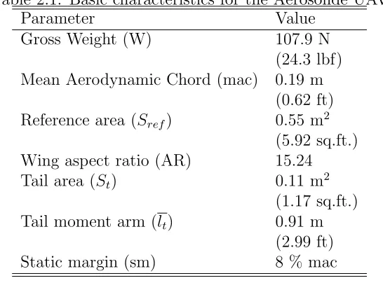
The basic characteristics of the Aerosonde are listed in Table 2.1, and the UAV is assumed to have the wing-tail planform as shown in Fig. 2.1. The AeroSim10

(21)

Table 2.1: Basic characteristics for the Aerosonde UAV.

Parameter Value

Gross Weight (W) 107.9 N (24.3 lbf) Mean Aerodynamic Chord (mac) 0.19 m

(0.62 ft) Reference area (Sref) 0.55 m2

(5.92 sq.ft.) Wing aspect ratio (AR) 15.24 Tail area (St) 0.11 m2

(1.17 sq.ft.) Tail moment arm (lt) 0.91 m

(2.99 ft) Static margin (sm) 8 % mac

1.448 m

0.1899 m

0.912 m

0.442 m

0.123 m

Figure 2.1: Planview showing the right-side geometry of the wing and tail for the Aerosonde UAV used in this paper.

(22)

2.2 Calculating the Adaptive Surface

Characteristics

The AeroSim blockset is a general-purpose blockset for dynamic simulations of an aircraft. The aircraft model in this blockest was modified for the current research to handle an adaptive wing. Relations from thin airfoil theory (TAT) were used to assist with modeling of the adaptive wing. The background for TAT is presented in Appendix A and relations used will be discussed in more detail in both Chapters 3 & 4.

One of the required parameters for modeling a trailing-edge flap in TAT is the hinge-line location. The adaptive surface, for the Aerosonde aircraft, was chosen to be a full-span flap at 80 % of the chord (xf/c). This is supplied in the

configuration file and then converted to an angular (θf) position using Eq. 2.1.

This angular coordinates are used in TAT modeling.

θf = cos

−1

1₋2xf c

(2.1)

Aside from the angular position of the hinge line it is also necessary to deter-mine the new change in lift (CL_δf) and the change in pitching moment coefficients

(CM_δf) due to adaptive surface deflections. Using the following equations the

co-efficients for lift and pitching moment for the adaptive flap can be determined: The following two equations represent the effects of the flap on the airfoil.

Cl_δf = [2(π−θf) + 2 sinθf] (2.2)

Cm_δf = [

1

4sin 2θf − 1

2sinθf] (2.3)

(23)

For this aircraft the assumption was made that the adaptive surface is a full span flap.

CL_δf = 0.9(Kf)(Cl_δf)

Sf lapped

Sref

(2.4)

CM_δf =Cm_δf −η(VH)(CL_αt)(−

∂ ∂δf

) (2.5)

∂ ∂δf ≈

2CL_δf

πAR (2.6)

Where Kf = 0.9 and Sf lapped/Sref = 1 for the full span flap.

Using these equations, the flap terms in the configuration script were modified to account for the adaptive wing.

2.3 Determining The Aircraft Drag Buildup

(24)

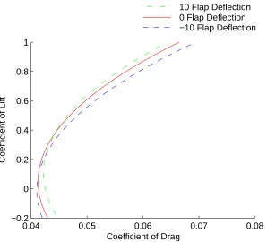
0.04 0.05 0.06 0.07 0.08 −0.2

0 0.2 0.4 0.6 0.8 1

Coefficient of Lift

Coefficient of Drag

−10 Flap Deflection 0 Flap Deflection 10 Flap Deflection

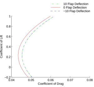
Figure 2.2: Demonstration of the drag polar shift due to a change in the flap angle for the AeroSim method (Eq. 2.7).

CD = CD0+

2(CL−CL0)

πARe +CDδf|δf| +CD_δe|δe|+CD_δa|δa|

+CD_δr|δr|+CDMM (2.7)

(25)

presented for the adaptive airfoil in Fig. 1.1(b). The drag polar now shifts both vertically and horizontally for a flap deflection. This demonstrates an increase in the LDR region for the adaptive wing. However, for this model the LDR is not as pronounced as the one shown for the airfoil in Chapter 1.1, which occurs for two reasons. First the Aerosonde aircraft is not specifically designed for an adaptive wing and secondly the drag coefficient of the fuselage andK2D term were directly

derived from the AeroSim model. Therefore this new method more accurately models the expected drag polar shifts for the adaptive aircraft but does not show substantial benefits of the adaptive flap.

CD = CD0 +K2D(CL−CLmind−2 sin(θf)δf)2

+(CL)

2

πARe +CD,f us+CDδe|δe|

(26)

0.04 0.05 0.06 0.07 0.08 −0.2

0 0.2 0.4 0.6 0.8 1

Coefficient of Lift

Coefficient of Drag

−10 Flap Deflection 0 Flap Deflection 10 Flap Deflection

(27)

Chapter 3 Static Longitudinal Stability

Analysis

The first logical step in investigating the effects of an auto-adaptive wing on the stability of an aircraft is a static stability analysis. This chapter will present the methodology and the results of this analysis. The methods described in this chapter are a combination of traditional stability equations and applications of thin airfoil theory.

The static analysis and results are presented in the following three sections:

1. Section 3.1 presents the static stability characteristics of the modified Aerosonde aircraft. There will also be a brief discussion of the effects of the flap on the CM_δf of the aircraft.

2. Section 3.2 presents the effect of an automated cruise flap on an airfoil. This is used to help explain the expected behavior the adaptive wing will have on the aircraft.

(28)

3.1 Aircraft Analysis

The first step in the aircraft analysis was to determine if the aircraft is statically stable. This typically is done by looking at the CMα curve for the aircraft. The following method describes the process of evaluating the static stability. The aircraft CM,cg vs. α variation for this case was constructed by first calculating

the CL and the downwash angle () at the tail for a given α. It is assumed that

the primary contribution to the aircraft CL comes from the wing CL. Using the

notation of Etkin and Reid,11 _{the following equations are obtained.}

CL=CL,0+ ∂CL

∂α α (3.1)

_≈ 2CL

πAR (3.2)

CL,t=

∂CL,t

∂αt

(αw−iw−+it) +

∂CL,t

∂δe

δe (3.3)

CM,cg =CM,ac,wb+CL(h−hn,w)−ηVHCL,t+CM,p (3.4)

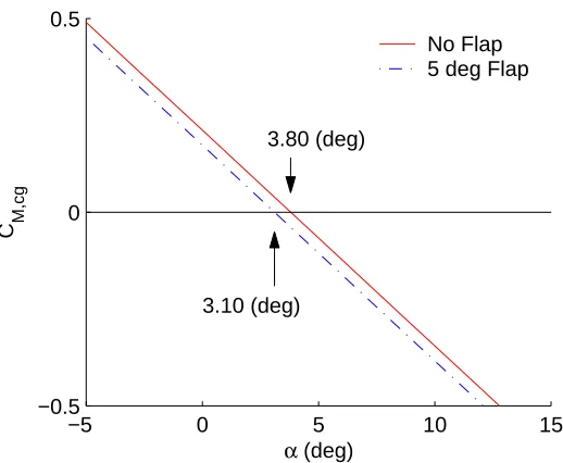
The resulting aircraftCM,cg vs.αvariation for two flap settings and for a fixed

elevator angle is shown in Fig. 3.1. The negative slope for the CM-α curves show

that the aircraft is statically stable and very traditional results are achieved. These two values were chosen to compare with the results from the dynamic stability studies and will be discussed in Chapter 4.

(29)

−5 0 5 10 15 −0.5

0 0.5

C M,cg

α (deg) 3.80 (deg)

3.10 (deg)

No Flap 5 deg Flap

Figure 3.1: CM,cg vs. α comparison for fixed elevator for two flap settings.

remember that this term is calculated about the reference point which for this aircraft is the aerodynamic center of the wing. The effects the two terms of the CMδf equation have on the stability can give some insight to the possible response of an aircraft to the automated adaptive wing. To briefly investigate these two components the wing-only and wing-tail combined effect will be examined.

At first only the wing component of Eq. 2.5,which is the first term Cmδf, is considered. It is well know that a positive flap deflection will increase the nose down pitching moment for an airfoil. That would lead to reason that the wing-only contribution would tend to pitch nose down after a positive flap deflection and vise versa for the negative deflection. For any flap deflection the wing-only contribution has a stabilizing effect on the aircraft. This does not mean however pitching moment of the wing-only contribution would be the required amount to re-trim the aircraft for steady flight with the new flap setting.

(30)

phe-nomenon occurs with the second term of Eq 2.5. When a flap is positively deflected there is an increase in the CL of the aircraft, which corresponds to a increase in

the downwash at the tail of the aircraft. This effectively decreases the α the tail experiences and thus decreases the nose down pitching moment the tail creates. This counteracts the wing-only contribution and thus makes the stabilizing effects of the wing-tail configuration less effective. This is only a brief description of the effects the adaptive wing would have on the stability of an aircraft.

3.2 Airfoil Analysis

To examine the static stability of an aircraft with an automated cruise flap, it is useful to study the stability of the flap controller on an airfoil. The function of the flap controller is to set the flap angle so that the airfoil is operating within the low-drag range. When the automation is done using sensed pressures, as described in Sec. 1.1.2, the flap controller adjusts the flap angle with the aim of getting the ∆C0

p to the target value. At this condition, the airfoil is said to be operating at

its ideal condition for that flap angle and the stagnation point is at the optimum location at the leading edge.

For the purpose of stability analysis and simulations, it is necessary to model the sensor inputs to the flap controller. A convenient approach to developing such a model is to use relations from thin airfoil theory for the ideal Cl and idealα for

an airfoil with a trailing-edge flap. These relations are shown in Eq. 3.5 and 3.6 for an airfoil with a flap angle of δf, with all angles in radians.

Clideal =Clideal,δf=0+ 2δfsinθf (3.5)

αideal =−

π₋θf

(31)

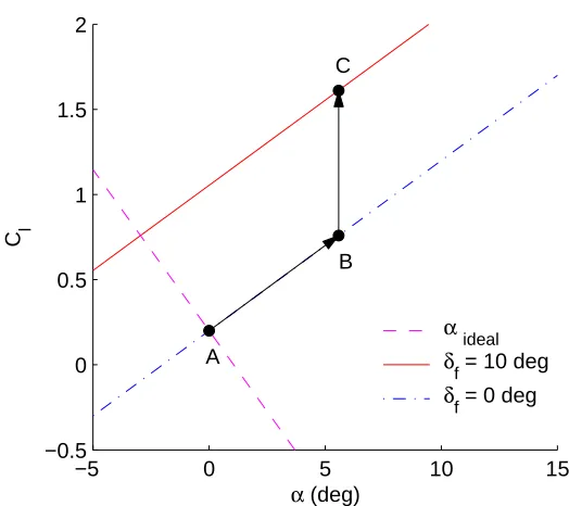
−5 0 5 10 15 −0.5

0 0.5 1 1.5 2

C l

α (deg) A

B C

δ_f = 0 deg

δ_f = 10 deg

α_ideal

Figure 3.2: Airfoil Cl vs. α curve for two flap angles to illustrate flap-controller

behavior.

Thus, an appropriate model for the fast-reacting flap controller could be one that uses the measured Cl of the airfoil and determines the desired flap angle for

that Cl:

δf =

Cl−Clideal,δf=0 2 sinθf

(3.7)

Figure 3.2 shows the Cl-α curves for a typical airfoil for two flap angles along

(32)

examined. When the system is perturbed to point B, theClincreases. As a result

the flap controller reacts by increasing the flap angle, as per Eq. 3.7. The result of the increase in flap angle is that the operating point now shifts to C, which is at a higher Cl. By carrying out this argument further, it is clear that the flap angle

will quickly diverge until it reaches the maximum deflection. Thus, it is seen that the flap controller is unstable.

In order to make this system stable, a controller is needed that will adjust the α in order to maintain a target Cl. It is for this reason, that the wind-tunnel

experiments of an airfoil with an automated cruise flap system, described in Ref. 4, used a controller in which both the flap angle andα were simultaneously adjusted at every time step to maintain desired values of ∆C0

p andCl. In a similar manner,

an automated cruise flap system implemented on an aircraft wing will need an accompanying system for control of α to maintain the desired CL. This control

of α is best achieved by adjusting the elevator to maintain the desired CL. Thus

an automated cruise flap system on an aircraft needs to be integrated with some form of trim controller in order for the entire system to be stable and achieve the desired response.

3.3 Summary of Static Stability Results

First the static stability and control characteristics were studied for an aircraft with a trailing-edge flap on the wing. When the flap is fixed at a specified angle, the stability characteristics are similar to those of a conventional aircraft. Also observed were the characteristics of both components of theCM_δf equation. It was

(33)

(34)

Chapter 4 Dynamic Longitudinal Stability

Analysis

The dynamic stability and control analysis was performed using conventional con-trol methods. The models and block diagrams used for this analysis were built using the AeroSim blockset10 _{in the Simulink environment. This blockset contains}

the complete nonlinear six degree-of-freedom (6-DOF) aircraft models and other supporting blocks that allow for accurate modeling of the aircraft dynamics. The focus of the effort was on the longitudinal dynamics, and only symmetric flight was considered. The UAV, shown earlier in Fig. 2.1, was used for this analysis and different approaches were studied for automating the adaptive wing.

The dynamic analysis and results are presented in the following five sections:

1. Section 4.1 presents the dynamic stability characteristics of the modified Aerosonde aircraft. There will also be a brief background into the lineariza-tion method used for the AeroSim non-linear model and how it compared to conventional linear control theory.

(35)

comparing the steady-state response to the predictions of the static-stability analysis, thus proving the validity of using the open loops for controller design.

3. Section 4.3 presents the various controllers that were developed for this investigation. It will also provide the two controller schemes for controlling the flap and elevator angles.

4. Section 4.4 presents the closed-loop simulations that were performed to in-vestigate the effects of the automated cruise flap. This will provide the insight to the implementation of the automated cruise flap on an aircraft.

5. Section 4.5 presents the results and finding of the dynamic simulations. It will reinforce the benefits of the various implementation schemes and their effect on the stability of the aircraft.

4.1 Dynamic Stability and Linearization

To understand the effects the automated flap will have on the dynamics of the aircraft it is first important to check the dynamic stability of the aircraft. This is performed so the effects of the flap can be isolated from any undesirable char-acteristics of the baseline aircraft. A traditional approach was used in which the aircraft was trimmed for various steady flight conditions and then analyzed for the appropriate stability characteristics and handling qualities.

(36)

the aircraft itself was dynamically stable and had level-one handling qualities for the flight conditions where the adaptive wing is of interest. It was also determined that the aircraft was controllable and observable.

The script that was developed from conventional methods was compared to the linearization script that came packaged with the AeroSim blockset. The script provided with AeroSim linearized the non-linear model about a specific set of flight conditions. This script also developed a state-space model that could be compared to the previous method. Although both models compared favorably the linearization script that was packaged with AeroSim matched closer to the response of the nonlinear models, which will be discussed in the following section.

4.2 Open Loop Simulations

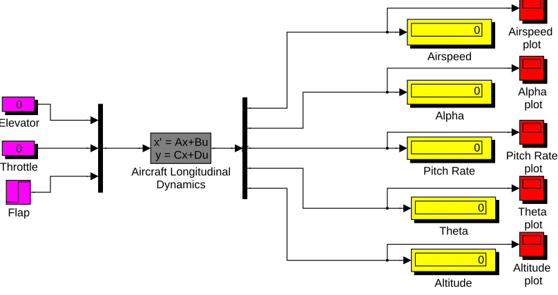
Having determined that the aircraft is dynamically stable, controllable, and ob-servable it was of interest to see how the aircraft would respond to an input to the adaptive flap. For this several open-loop models were developed to compare and validate the longitudinal model for the UAV. The results from the open-loop simulations were compared with those from the static stability analysis. Fig. 4.1 shows, as an example, the nonlinear model used for determining the response to a step input to the flap angle. Linear models for the longitudinal motion were derived from the 6-DOF model for designing the various controllers that will be described in the following section. The block diagram for studying the open-loop response to the flap using the linear model is shown in Fig. 4.2.

(37)

[0 0 0] Winds 13 Throttle Theta Plot 0 Theta STOP Stop Simulation when A/C on the ground 0 Rudder 0 Reset Pitch Rate Plot 0 Pitch Rate 13 Mixture 1 Ignition Flap 13 Elevator Demux Demux Demux Bank Angle Aileron

Bank Angle PI Controller

Altitude Plot 0 Altitude Alpha Plot 0 Alpha Airspeed Plot 0 Airspeed Controls Winds RST States Sensors VelW Mach Ang Acc Euler AeroCoeff PropCoeff EngCoeff Mass ECEF MSL AGL REarth AConGnd

6 DOF UAV

Figure 4.1: Nonlinear open-loop model for studying the step response to the flap angle. 0 Throttle Theta plot 0 Theta Pitch Rate plot 0 Pitch Rate Flap 0 Elevator Demux Altitude plot 0 Altitude Alpha plot 0 Alpha Airspeed plot 0 Airspeed

x’ = Ax+Bu y = Cx+Du Aircraft Longitudinal

Dynamics

(38)

0 100 200 300 0

1 2 3 4 5 6

Flap angle (deg)

Time (s)

(a)

0 100 200 300

18 19 20 21 22 23 24

Velocity (m/s)

Time (s)

(b)

0 100 200 300

2.5 3 3.5 4

Alpha (deg)

Time (s)

(c)

Static Nonlinear Linear

Figure 4.3: Comparison of Linear, Nonlinear, and Static results.(a) Flap Angle,(b) Velocity response, and (c) Alpha response.

of the two open-loop simulations agree well with each other and with the results of the trimmed static stability calculations. This good agreement validates the use of the longitudinal linear dynamics model for use in controller design for the UAV.

4.3 Controller Design

(39)

model was to evaluate different options for incorporating the automated cruise flap. Because only the longitudinal motion is of interest, a bank-angle controller was incorporated to maintain zero bank angle. An altitude-hold and airspeed controller were also developed and incorporated to maintain the desired flight path. These controllers are shown in Fig. 4.4. The controllers were designed using conventional methods and the linear aircraft models were used for controller validation and robustness verification.

[0 0 0]

Winds

STOP

Stop Simulation when A/C on the ground 0 Rudder 0 Reset 13 Mixture 1 Ignition A/C CL Current Airspeed Desired Airspeed Flap Commanded

Elevator Commanded

Flap Control Method

0 Desired Altitude 30 Desired Airspeed Demux Demux Demux Bank Angle Aileron

Bank Angle PI Controller

Altitude

Desired Altitude Throttle

Altitude PID Controller

Controls Winds RST States Sensors VelW Mach Ang Acc Euler AeroCoeff PropCoeff EngCoeff Mass ECEF MSL AGL REarth AConGnd

6 DOF UAV

Figure 4.4: Model for closed loop simulation.

4.3.1 Bank, Airspeed, and Altitude Controllers

(40)

A proportional and integral (PI) controller was designed and implemented for maintaining zero bank angle.

With a controller to maintain zero bank angle, the next step was to maintain a desired forward airspeed. A proportional, integral, and derivative (PID) controller was used to close the airspeed to elevator loop. For the various flight conditions the appropriate gains were determined and implemented to maintain the desired response.

The last control loop required to maintain the desired flight conditions was an altitude hold. This loop was closed using a closed-loop throttle controller. A proportional controller was used to maintain the desired altitude-hold response. These three feedback controllers are used to maintain constant flight speed, alti-tude, and symmetric flight when the flap is dynamically adjusted for minimizing drag.

4.3.2 Flap and Elevator Controllers

As shown earlier, when an automated cruise flap is incorporated on an aircraft, there is a need for an accompanying controller that will maintain the desired aircraft CL. This CL control is best achieved by adjusting the elevator angle.

When changes are made to the flap angle, the elevator controller will then adjust the elevator to re-trim the aircraft at the desiredCL, thus maintaining the desired

(41)

2 Elevator Commanded

1 Flap Commanded

A/C CL Flap Angle

Automated Cruise Flap

Airspeed

Desired Airpseed Elevator

Airspeed PID Controller

3 Desired Airspeed

2 Current Airspeed

1 A/C CL

Figure 4.5: Flap and elevator controllers with no coupling.

Decoupled flap and elevator controllers

In this option, the controllers for the flap and elevator are independent, as shown in Fig. 4.5. The elevator controller is the PID controller described earlier that maintains the desired airspeed. The flap controller adjusts the flap angle in an effort to maintain the wing at its ideal condition, by shifting the drag polar of the wing. For the purpose of the simulation, the aircraftCL was used as input to the

flap controller to determine the ideal flap angle (δf) using Eq. 4.1. The relation

in Eq. 4.1 for the aircraft flap controller is similar to that shown earlier in Eq. 3.7 for the flap controller on an airfoil.

δf =

CL−CLideal,δf=0 2 sinθf

(4.1)

On an aircraft, the CL can be deduced from the measured airspeed. In the

current work, theCLused by flap controller at any instant was determined from a

windowed average of the measuredCL. The windowed average was taken over the

past 30 seconds of the simulation. This was done in order to prevent the flap from reacting to high-frequency CL oscillations. In addition, the model was designed

so that flap-actuation frequency was a user-specified variable.

(42)

1 Flap Angle

Trigger System

Rate Limiter Max Deflection

Limits

Enable System

A/C CL<L> delta_f out

Calculate Opt

Flap Angle Average

30 s Buffer 1 A/C CL

Figure 4.6: Exploded block diagram of the flap controller.

is then fed into a subsystem that can be enabled at sometime after the simulation is started to simulate the system being turned on during flight. After the system is switched on, it can be actuated at various frequencies using the trigger. When triggered, Eq. 4.1 calculates the optimum flap angle which is then rate limited and bounded by the limits of the maximum flap deflections. The final commanded flap deflection is then sent to the input of the aircraft model.

Coupled flap and elevator controllers

In the second option, the flap and elevator controllers were coupled. In order to automatically compensate for the trim changes due to flap. The flap-to-elevator coupling is illustrated in Fig. 4.7. For every change made to the flap angle, a change was automatically made to the elevator angle using a predetermined gain. This gain is aircraft specific. The sensitivity of this gain to changes in various parameters such as airspeed and cg shifts is unknown. However, for the simula-tions that were performed during this study it remained constant. This coupling was included in order to automatically compensate for the trim changes due to a dynamically-changing flap.

(43)

2 Elevator Commanded

1 Flap

Commanded _−K− Flap to Elevator Gain

A/C CL Flap Angle

Automated Cruise Flap

Airspeed

Desired Airpseed Elevator

Airspeed PID Controller

3 Desired Airspeed

2 Current Airspeed

1 A/C CL

Figure 4.7: Illustration of the flap-to-elevator coupling.

4.4 Closed Loop Simulations

The results of the dynamic simulations are presented for two cases. In the first case, the effect of the flap controller on the response of the aircraft is presented. The results are shown for both with and without the flap-elevator coupling. In the second case, the results are presented for the response of the aircraft to a step change in the desired airspeed. These results are presented for four differ-ent flap-actuation frequencies. The benefits of the auto-adaptive wing were also investigated.

4.4.1 Flap-Elevator Coupling Comparison Study

Figure 4.8 shows the response of the aircraft from a simulation in which the flap controller, that is initially off, is turned on at t = 120 s. The responses are compared for both with and without the flap-to-elevator coupling. In these simulations, the desired airspeed is set at 30 m/s for the entire duration. The flap angle is initially set to 0 deg and the flap controller is off. Att = 30 s, the aircraft reaches steady-state conditions, as shown in the plots in Fig. 4.8 (a).

(44)

0 100 200 300 29.4

29.6 29.8 30 30.2

Velocity (m/s)

Time (s)

(a)

0 100 200 300

0 1 2 3 4 5

Flap Angle (deg)

Time (s)

(b)

0 100 200 300

2 4 6 8 10

Elevator Angle (deg)

Time (s)

(c)

Decoupled

Flap−Elevator Coupling

Figure 4.8: Comparison of aircraft response with and without flap-elevator cou-pling: (a) velocity, (b) flap angle, and (c) elevator angle

(45)

100 200 300 29 30 31 32 33 34 Velocity (m/s) Time (s) (a)

Flap switched on at 120 (s) 1/120 HZ Flap Actuation 1/30 HZ Flap Actuation 1 HZ Flap Actuation

100 200 300

0 1 2 3 4 5

Flap Angle (deg)

Time (s)

(b)

100 200 300

190 195 200 205 Altitude (m) Time (s) (c)

100 200 300

0.85 0.9 0.95 Throttle (%) Time (s) (d)

200 220 240 260 32.5 33 33.5 Velocity (m/s) Time (s) (e)

Zoomed in view of velocity and throttle

200 220 240 260 0.91 0.92 0.93 0.94 Throttle (%) Time (s) (f)

(46)

4.4.2 Change in Desired Airspeed

In the second case study, the effect of a step input to the desired airspeed is studied for different flap-actuation frequencies. In this simulation, the airspeed is initially set to 30 m/s with the flap set to zero deg and the flap controller turned off. At t = 120 s, the flap controller is switched on and the aircraft is allowed to reach steady-state conditions. Subsequently, att = 200 s, a step input is given to the desired airspeed to change it to 33 m/s. The response plots for the velocity and flap angle are presented in Figs. 4.9(a),(b) for four different flap-actuation frequencies.

It is seen that for all the four actuation rates, the aircraft responds to the change in desired velocity by adjusting the flap angle appropriately and settles quickly to the new steady-state condition. When the flap is actuated at high frequency (every 1 s), the response is smoother than when the flap is actuated at low frequency (every 120 s). In both cases, however, there is no undesirable behavior. These response plots confirm that as long as there is a controller that adjusts the elevator angle to maintain the desired airspeed, the automated cruise flap system is successful in continuously setting the optimum flap angle on the wing without any undesirable flight characteristics.

4.4.3 Benefits of Adaptive Wing

(47)

100 200 300 0 5 10 15 20

Flap Angle (deg)

Time (s)

New Drag Model

(a)

Flap switched on at 120 (s)

100 200 300

0.04 0.045 0.05 0.055 0.06

Coefficient of Drag (C

D

)

Time (s) (b)

100 200 300

0.26 0.28 0.3 0.32 0.34 0.36 Throttle (%) Time (s) (c)

100 200 300

0.08 0.085 0.09 0.095 0.1

Fuel Consumption (kg/hr)

Time (s) (d)

100 200 300

10 15 20 25 30 Velocity (m/s) Time (s) (e)

100 200 300

195 200 205 Altitude (m) Time (s) (f)

Figure 4.10: Demonstration of drag benefits of the adaptive aircraft during sim-ulation. The figures are: (a) flap deflection, (b) Coefficient of Drag (CD), (c)

(48)

in Fig. 4.10 (b), for the aircraft was plotted versus time to demonstrate that the drag is reduced after the automated flap optimizes the wing. Figure 4.10 (c) shows the throttle reduction after the flap system is switched on. Much like the throttle, there is also a reduction in the fuel consumption indicating that the aircraft with the adaptive wing is indeed operating more efficiently at the same desired flight condition. From these plots it is clear that the auto-adaptive aircraft has drag benefits. The drag savings can be increased if the aircraft and airfoil are tailored for wing adaptation. Such a decrease in drag translates to a large benefit on the range, endurance, andVmax of an aircraft. Future work in this area could provide

a better understanding of the aircraft drag with a auto-adaptive aircraft.

4.5 Summary of Dynamic Stability and

Control Results

In the interest of better understanding the effects of an adaptive wing on an aircraft, a dynamic stability and control analysis was performed. As described in this chapter, a number of non-linear closed loop models were studied. Two controller schemes were developed for comparing the effects of re-trimming the aircraft after a change in the adaptive flap. It was observed that if the elevator was automatically deflected for every flap defection by some predetermined amount a more desirable response was achieved. When the flap was not coupled to the elevator, the aircraft took longer to re-trim after changes in the flap, although the response was still quite acceptable.

(49)

condition. The system therefore responded appropriately to changes to the desired flight conditions.

(50)

Chapter 5 Concluding Remarks

5.1 Summary of Results

With increasing interest in the use of adaptive lifting surfaces for improved air-craft performance, it is of interest to study the airair-craft stability and control char-acteristics with adaptive wings. This work builds on a recent development of an automated cruise flap for adapting an airfoil to achieve low drag over a large lift range. Such an automated cruise flap system was shown to have unusual lift and pitching moment curves, which prompted the need for studying the effect on aircraft stability and control. Therefore an aircraft was selected and analyzed to determine the effects the adaptive wing on the aircraft stability and control.

(51)

accompanying elevator controller to maintain the desired airspeed.

In the second part of the research effort, dynamic analysis and simulations were conducted using Simulink and the AeroSim blockset. The dynamic models were validated by verifying that the steady-state results from open-loop simulations agreed with the results of the trim conditions from the static-stability analysis. Two schemes were developed for the flap and elevator controllers. In the first scheme, there is no coupling between the flap controller and that for the elevator. In the second scheme, flap-elevator coupling was achieved by making a change to the elevator angle using a predetermined ratio whenever the flap controller makes a change to the flap angle.

The results of the simulations show that the automated flap is successful in ad-justing the flap angle when accompanied by an elevator controller that maintains the desired airspeed. However, a small velocity spike was observed when the flap controller was switched on. When flap-elevator coupling was used, this velocity spike was eliminated. The flap and elevator controllers were also successful in tracking changes to the desired airspeed and no undesirable behavior was noticed for a wide range of flap actuation frequencies. The benefits of this type of system were also captured while performing the dynamic analysis. These results provide confidence in the implementation of the automated-flap concept on an aircraft wing.

(52)

5.2 Recommendations for Future Work

While studying the effects of the adaptive aircraft a few areas of interest for future investigation have surfaced. The following three topics would be areas to investigate in more depth:

1. First an investigation into the drag buildup and modeling, which is one area where improvements can be made to more accurately model an aircraft with an adaptive wing. As shown in Section 2.3, the drag polar did not shift as expected for an aircraft with an adaptive wing and required a new model to be developed for this investigation. There are also questions about the differences in fuselage profile drag for an aircraft without and with an adaptive wing.

2. Second it would be useful to study an aircraft that is specifically designed for this technology. The Aerosonde was not specifically designed for this type of technology and there were some assumptions made to determine aircraft performance. An aircraft that is designed for this type of technology would be more successful in showing the benefits of the adaptive wing. To get a better idea of the benefits of the adaptive wing, a complete aircraft model would have to be created for an aircraft designed for the adaptive wing.

(53)

Chapter 6 References

1 _{Stanewsky, E., “Aerodynamic benefits of adaptive wing technology,”}_Aerospace Science and Technology, Vol. 4, 2000, pp. 439–452.

2 _{Monner, H. P., Breitbach, E., Bein, T., and Hanselka, H., “Design aspects of}

the adaptive wing — the elastic trailing edge and the local spoiler bump,” The Aeronautical Journal, February 2000, pp. 89–95.

3

McGhee, R. J., Viken, J. K., Pfenninger, W., Beasley, W. D., and Harvey, W. D., “Experimental Results for a Flapped Natural-Laminar-Flow Airfoil with High Lift/Drag Ratio,” NASA TM 85788, May 1984.

4 _McAvoy, _C. _W. _and _{Gopalarathnam,} _A., _“Automated

Trailing-Edge Flap for Airfoil Drag Reduction Over a Large Lift-Coefficient Range,” AIAA Paper 2002–2927, June 2002, available from http://www.mae.ncsu.edu/homepages/ashok/pubs/AIAA-2002-2927.pdf.

5

McAvoy, C. W. and Gopalarathnam, A., “Automated Cruise Flap for Airfoil Drag Reduction Over a Large Lift Range,” Journal of Aircraft, Vol. 39, No. 6, November–December 2002, pp. 981–988.

6 _{Drela, M., “XFOIL: An Analysis and Design System for Low Reynolds Number}

(54)

of Lecture Notes in Engineering, Springer-Verlag, New York, June 1989, pp. 1–12.

7 _{Pfenninger, W., “Investigation on Reductions of Friction on Wings, in}

Partic-ular by Means of Boundary Layer Suction,” NACA TM 1181, August 1947.

8 _{Somers, D. M., “Design and Experimental Results for a Flapped}

Natural-Laminar-Flow Airfoil for General Aviation Applications,” NASA TP 1865, June 1981.

9 _{Gopalarathnam, A. and McAvoy, C. W., “Effect of Airfoil Characteristics on}

Aircraft Performance,” Journal of Aircraft, Vol. 39, No. 3, May–June 2002, pp. 427–433.

10 _{Niculescu, M.,} _{AeroSim blockset: User’s Guide}_{, Unmanned Dynamics, LLC,}

No. 8 Fourth St., Hood River, OR 97031, http://www.u-dynamics.com.

11

Etkin, B. and Reid, L. D., Dynamics of Flight, John Wiley and Sons, Inc., 3rd ed., 1996.

12 _{Katz, J. and Plotkin, A.,} _{Low-Speed Aerodynamics}_{, Cambridge University}

(55)

Appendix A

Thin Airfoil Theory Analysis

This appendix briefly presents the thin airfoil theory calculations used in the modeling of the auto-adaptive wing.

It is well known12 _{that the total circulation, Γ, of an airfoil can be calculated}

from thin airfoil theory using Eg. A.1.

Γ = Z c

0 γ(x)dx (A.1)

Using the coordinate transformation shown in Eq. A.2 the total circulation be-comes Eq. A.3.

x= c

2(1−cosθ) (A.2)

Γ = c 2

Z π

0 γ(θ)sinθdθ (A.3)

Where γ(θ) can be presented a the Fourier series shown in Eg. A.4.

γ(θ) = 2V∞[A0

1 + cosθ sinθ +

∞ X

n=1

Ansinnθ] (A.4)

(56)

deflections, the Fourier coefficients can be calculated from Eqs. A.5 and A.6.

A0 =α+

1 π

Z π

θf

δfdθ =α+

δf

π(π−θf) (A.5)

An =−

2 π

Z π

θf

δfcosnθdθ =

2δf

π

sinnθf

n (A.6)

Whereδf andθf are the flap angle and flap hinge location, respectively, in radians.

It also turns out from thin airfoil theory that the approximate Cl of the airfoil

can be calculated from only the first two coefficients using Eq. A.7.

Cl= 2πA0+πA1 (A.7)

Finally, to compute the Clideal corresponding to the angle-of-attack at which the

stagnation point is located exactly at the leading edge of the thin airfoil, one must find the Cl where there are no singularities (or infinite suction peaks) on either

the upper or lower surface. This Clideal corresponds to the Cl where the Fourier

coefficient, A0, goes to zero. Thus the Clideal can be calculated using Eq. A.8.

(57)

Appendix B

Linear Longitudinal Dynamic

Stability Analysis Script

This appendix briefly presents the construction of the states based model and the stability analysis that was created from traditional stability calculations.

% Longitudinal Dynamic Analysis

% 2-10-04

% Victor Vosburg

% Inputs

load aerosondecfg.mat

U0= 30; % Flight Velocity (consistent units with config file m/s) m=11;

gamma=1.4;

R=287; %J/(kg K)

T=286.85; %Standard Day asound=339.53;

M=U0/asound;

rho=1.2017; %density sea level Q= 1/2*rho*U0^2;

alpha=0; AR=b^2/S;

g=9.81; %gravity m/s^2 IC=[0 0 0 0]

(58)

alpha=1.31*pi/180; deltae=0.0404; deltaf=0;

CLREF=CL0+CLa*alpha+CLdf*deltaf+CLde*deltae+CLM*M; CDREF=CD0+(CLREF-CL0)^2/(pi*osw*AR)+CDdf*deltaf ...

+CDde*deltae+CLM*M;

% Calculate A MATRIX

% X Forces

Xu=-(M*CDM+2*CDREF)*Q*S/(m*U0);

Xw=-((2*CLREF*CLa/(pi*osw*AR))-CLREF)*Q*S/(m*U0);

% Z Forces

Zu=-(M^2/(1-M^2)*CLREF+2*CLREF)*Q*S/(m*U0); Zw=-(CLa+CDREF)*Q*S/(m*U0);

Zwdot=-CLalphadot*MAC*Q*S/(2*U0*U0*m); Za=U0*Zw;

Zadot=U0*Zwdot;

Zq=-CLq*MAC*Q*S/(2*U0*m);

% Moments

Mu=CmM*M*Q*S*MAC/(U0*Iy); Mw=Cma*Q*S*MAC/(U0*Iy);

Mwdot=Cmalphadot*MAC*Q*S*MAC/(2*U0*U0*Iy); Ma=U0*Mw;

Madot=U0*Mwdot;

Mq=Cmq*MAC*Q*S*MAC/(2*U0*Iy);

A=[Xu Xw 0 -g;... Zu Zw U0 0;...

Mu+Mwdot*Zu Mw+Mwdot*Zw Mq+Mwdot*U0 0; ... 0 0 1 0];

% Calculated B matrix

% X forces

Xde=-CDde*Q*S/m; Xdf=-CDdf*Q*S/m; Xdt=0;

% Z forces

(59)

Zdf=(-CLdf)*Q*S/m; Zdt=0;

% Moments

Mde=Cmde*Q*S*MAC/Iy; Mdf=Cmdf*Q*S*MAC/Iy; Mdt=0;

B=[Xde Xdf Xdt; ... Zde Zdf Zdt; ... Mde Mdf Mdt; ... 0 0 0];

%C and D matrices

C=[1 0 0 0;0 1 0 0;0 0 1 0;0 0 0 1]; D=[0 0 0;0 0 0;0 0 0;0 0 0];

long=ss(A,B,C,D) damp(long)

co=ctrb(long); ob=obsv(long);

The Stability and Control of an Aircraft with an Adaptive Wing

ABSTRACT

The Stability and Control of an Aircraft with an

Adaptive wing

To all my friends and family

BIOGRAPHY

ACKNOWLEDGEMENTS

Table of Contents

List of Tables

List of Figures

Nomenclature

Chapter 1

Introduction

1.1

Background

1.1.1

Airfoil Adaptation Using a Camber-Changing TE

Flap

1.1.2

Recent Auto-Adaptive Airfoil Research at NCSU

1.1.3

Issues for Aircraft Stability and Control

1.2

Research Motivation & Objectives

1.3

Brief Outline

Chapter 2

Aircraft Characteristics

2.1

Aircraft Configuration

2.2

Calculating the Adaptive Surface

Characteristics

2.3

Determining The Aircraft Drag Buildup

Chapter 3

Static Longitudinal Stability

Analysis

3.1

Aircraft Analysis

3.2

Airfoil Analysis

3.3

Summary of Static Stability Results

Chapter 4

Dynamic Longitudinal Stability

Analysis

4.1

Dynamic Stability and Linearization

4.2

Open Loop Simulations

4.3

Controller Design

4.3.1

Bank, Airspeed, and Altitude Controllers

4.3.2

Flap and Elevator Controllers

4.4

Closed Loop Simulations

4.4.1

Flap-Elevator Coupling Comparison Study

4.4.2

Change in Desired Airspeed

4.4.3

Benefits of Adaptive Wing

4.5

Summary of Dynamic Stability and

Control Results

Chapter 5

Concluding Remarks

5.1

Summary of Results

5.2

Recommendations for Future Work

Chapter 6

References

Appendix A

Thin Airfoil Theory Analysis

Appendix B

Linear Longitudinal Dynamic