SOIL STRUCTURE INTERACTION ANALYSES FOR MODELING
NONLINEAR RESPONSE OF DIRECT-SHEAR TYPE TESTS
Dhrubajyoti Datta1, Amit Varma2
1 Graduate Research Assistant, Purdue University, West Lafayette, IN-47907 2 Professor, Purdue University, West Lafayette, IN-47907
ABSTRACT
The behaviour of the interface between the structure and soil has substantial influence on the response of critical infrastructure systems, due to the presence of material and geometric nonlinearities. The article focuses on modelling direct shear-type tests for a concrete foundation sliding on Ticino sand confined in a chamber under continuous confining pressures. The foundation is subjected to cyclic displacement-controlled load packets of gradually increasing amplitudes. The force-displacement response from the analytical SSI models will be compared with the experimental data. The behaviour of the interface is modelled through a non-linear soil model as well as contact interaction methods; and a comparison will be made between the two approaches.
INTRODUCTION
The dynamic soil structure interaction analysis of nuclear structures and components during a seismic event is currently carried out using the equivalent linear analysis in the frequency domain (ELFD). The ASCE 4-1998 [1] lays down a detailed set of instructions to perform the linear SSI analysis in the frequency domain. While the ELFD method produces acceptable results for low to medium scale seismic events and helps in assigning damping parameters of the structural response in accordance with the strong motion frequency ranges, it falls short of accounting for the material and geometric nonlinearity at the interface. Furthermore, the failure of the structure cannot be analysed with certainty owing to the cyclic and kinematic nature of seismic excitation.
The modelling of the non-linear soil parameters is a key prerequisite to model the behaviour of the soil-structure interface to seismic excitation. Although there is a plethora of sophisticated constitutive models in literature to model the soil domain, their utilization is limited because (i) they require a large number of parameters for calibration which is numerically intensive (ii) the test data needed for calibration from dynamic resonant column tests, torsional shear tests, dynamic direct shear tests are not easily available for most soil types. Hence, it is essential to limit the number of parameters for a constitutive model while ensuring the fundamental material properties need for the material model are easily available for most soil types. The non-linear time domain SSI analysis method discussed in this paper utilizes linear elastic material parameters to develop a non-linear multistep hysteretic model which can be easily performed in commercial FEA tools like ABAQUS or LS DYNA. Consequently, the hysteretic response is obtained from the post-yielding shear stress vs. shear strain behaviour.
The article focuses on simulating the nonlinear force-displacement response of shallow foundations subjected to cyclic loading. The material model is encoded in ABAQUS through a user subroutine and validated against a series of large scale, cyclic loading tests on shallow foundation resting on cohesionless soil, carried out at the European Laboratory for Structural Analysis (ELSA) under the TRISEE project [2]. The objective of the analytical study is to compare the load-displacement response of the soil-foundation assembly to realistically formulate a non-linear time domain SSI approach taking interfacial non-linearities into consideration.
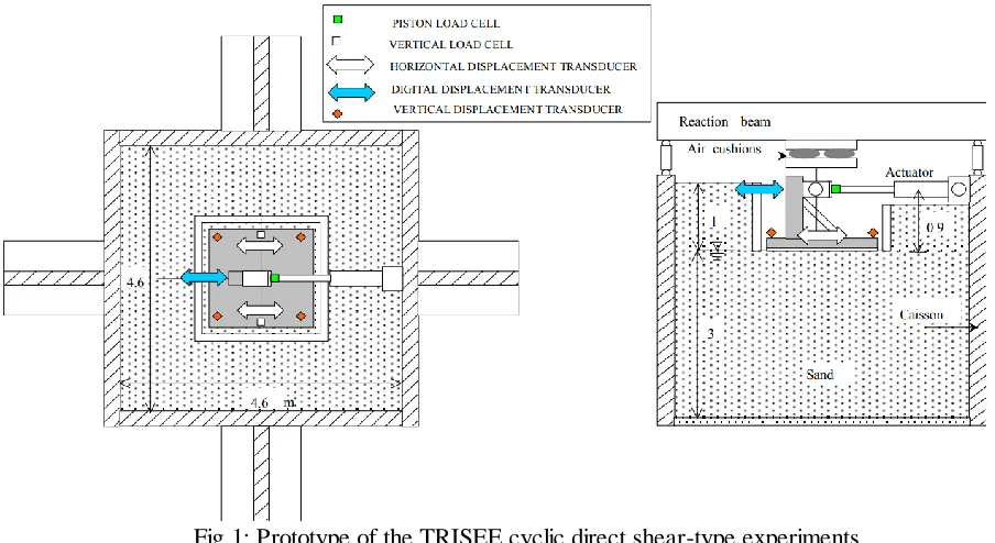
DESCRIPTION OF THE TRISEE EXPERIMENTS
experiments for high density sands are used for comparison of the numerical models to the experimental data.
Fig 1: Prototype of the TRISEE cyclic direct shear-type experiments
MULTILINEAR INELASTIC HYSTERETIC SOIL MATERIAL MODEL
The non-linear soil is modelled using a. inelastic hysteretic soil model in ABAQUS [4]. The soil model is comprised of a shear stress-strain backbone curve and the material damping is represented through the post-yielding shear stress vs. shear strain behaviour. The first point of the backbone curve is (0, 0) by default while the other stress-strain pairs individually represent an elastic-perfectly plastic “layer” with varying yield stress-strain values. The response of the all these individual layers is summed up to generate a post-yielding shear stress vs shear strain curve which is valid for a single hydrostatic stress in the element.
The backbone curve is applicable at the confinement or reference pressure at which the
experiments were performed. Besides the backbone curve and the reference pressure (
p
ref), the
constitutive model includes pressure sensitivity parameters (
a
0, a
1,a
2 andb
), dilation constants and
cut-off pressure (
p
0); which can be calibrated from experimental data. The stress-strain behaviour
of Ticino sands were obtained from a set of resonant column and monotonic loading torsional
shear tests [5, 6] on solid cylindrical specimens isotropically consolidated at varying void ratios .
The shear modulus from the tests was plotted against the log of shear strain, and a well-defined
plateau was observed for the shear modulus, G at strains less than 0.001%. This data was used to
obtain the shear strain vs shear stress backbone curve for the TRISEE experiments. The reference
pressure was scaled up with respect to the operating pressure (p) of the experiment and the datum
pressure (p0) as (LS DYNA)
𝜏(𝑝,
ϒ
)
𝜏(𝑝
𝑟𝑒𝑓,
ϒ
)
= √
[𝑎
0+ 𝑎
1(𝑝 − 𝑝
0) + 𝑎
2(𝑝 − 𝑝
0)
2]
[𝑎
0+ 𝑎
1(𝑝
𝑟𝑒𝑓− 𝑝
0) + 𝑎
2(𝑝
𝑟𝑒𝑓− 𝑝
0)
2]
The dependence of the initial shear modulus on void ratio and confining stresses was defined on
the basis of resonant column tests [7] as
𝐺
0= 𝐶
𝑔. 𝐹(𝑒). 𝜎
𝑚′ 𝑛. 𝑝
𝑎1−𝑛where,
𝐶
𝑔= 710 Dimensionless soil constant
𝐹(𝑒) = (2.27 − 𝑒)
2/(1 + 𝑒)
Void ratio function (0.579 ≤ e ≤ 0.930)
n = 0.43
Modulus exponent
𝑝
𝑎Atmospheric pressure
𝜎
𝑚′Mean effective stress
The initial shear modulus at varying reference pressures was used to formulate the backbone curve.
The yield surface defined by each elasto-plastic layer (denoted by
i
) is defined in terms of the
second stress invariant, which is converted from the maximum shear stress as [8]
𝐽
2𝑖= (𝜎
𝐼′:
𝜎
𝐼′2
) <
4
3
𝜏
𝑚𝑎𝑥2The elastic shear and bulk modulus are pressure sensitive governed by the constants
a
0, a
1,a
2 andb
. The ratio between these values determine how the backbone curve is scaled when the hydrostatic
pressure changes during the simulation. The cutoff pressure
p
0determines the point below which
shear stresses are set to zero. In other words, when the current pressure goes below the cutoff
pressure, the soil has no stiffness in tension. However, for clayey soil or sticky interfaces, a
non-zero cutoff pressure might be helpful in replicating the normal stick slip behaviour.
FINITE ELEMENT MODELLING PROCEDURE
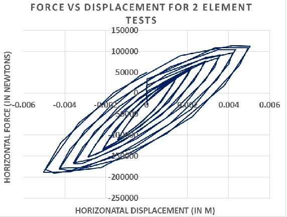
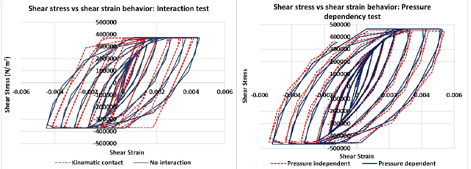
The primary motivation of the study is to compare numerical NLSSI results with the experimental data from the TRISEE experiments. The hysteresis behavior of the non-linear soil is generated by using a two-element finite element model which imitates the behavior of the linear elastic soil model. The reference pressure at the soil structure interface and the operating shear strain range for the displacement controlled load cycles is obtained from a linear SSI analysis without any material or geometric nonlinearity. The numerical backbone curve is derived from the experimental G/Gmax vs. ϒ curve, which is calibrated to mimic
a
2 were set to activate pressure dependency, such that the backbone curve could scale with the referencepressure.
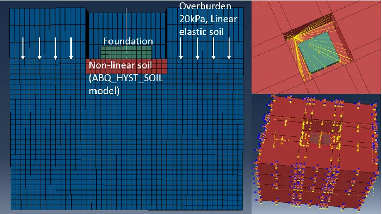
Fig 3: Finite element model of the TRISEE experimental prototype
A detailed model of the TRISEE experimental prototype is built with a layer of fine meshed non-linear soil surrounding the foundation (in red) which is tied to the surrounding soil domain, also non-non-linear in nature. The backbone curve for the underlying soil domain was scaled according the confinement pressure. The steel foundation and formwork have isotropic linear elastic properties. The loading is applied to the structure in terms of sine shaped displacement cycles of gradually increasing amplitude, through a rigid steel column which is embedded in the foundation. A constant uniform load of 300 kN is applied on top of the foundation and maintained throughout the simulation. The unsaturated layer of sand surrounding the foundation exerts an overburden pressure of 20 kPa and is retained through a 1m formwork surrounding the sand. This is simulated by constraining the nodes of the trench boundary surfaces to move together. The edges of the soil domain are fixed to ensure soil confinement.
Fig 4: Displacement-time loading history for sliding of foundation on high density sand
in terms of hourglass modes [4]. Excitation of the hourglass modes results in heavy mesh distortion, which is controlled by activating the stiffness control factor.
The interaction between the soil and structure is controlled by a softened contact overclosure relationship in the normal direction, in which the contact pressure is an exponential function of the clearance between the contact surfaces. The contact pressure increases exponentially as the clearance between the two surface decreases which captures the phenomenon of increasing soil stiffness for increased penetration. The tangential interaction is implemented through the non-linear interface elements and doesn’t require a friction based interaction model. However, an equivalent kinematic friction-based interaction model can be calibrated with the non-linear behavior of the soil-structure interface. It won’t be able to accurately capture the hysteresis behavior but would be effective in determining the margins of the non-linear dynamic response.