Hybrid Model for MRI Brain Image
Registration Using Rigid and Non Rigid
Techniques
N.Nandhagopal1, M.Karnan 2, Selvanayaki 3 Research Scholar, M.S.University, Tirunelveli, India1
Department of Computer Science and Engineering, Tamilnadu College of Engineering, Coimbatore, India2 Department of Computer Applications,Tamilnadu College of Engineering, Coimbatore, India 3
ABSTRACT: Image Registration is an important and challenging factor in the Medical Image Processing. This paper describes a new hybrid model for Image Registration through Magnetic Resonance Image (MRI). This model consists of three phases. In the first phase, film artifacts and unwanted portions of MRI Brain image are removed. . Secondly, the noise and high frequency components are removed using weighted median filter (WM). Finally, Hybrid model is applied for registration phase in which this phase comprises of two methods namely non-rigid and rigid. In non-rigid ,block based technique is implemented in which the reference image and normal images are split in to number of blocks of size 64×64.Each and every corresponding blocks from reference image and normal images are compared using Ant colony optimization(ACO).if the images are similar, the resultant image obtained is given to rigid method as input. In rigid method, similarity measures are calculated for the given image which includes 1. Contrast checking (CC) 2. Sum of Square Difference (SSD) 3.Calculation of White cells and 4.point mapping.
KEYWORDS: Magnetic Resonance Image (MRI), Brain tumor, Pre processing, Enhancement, Registration, Block Based, Similarity Measure, Rigid and Non -Rigid Technique.
I. INTRODUCTION
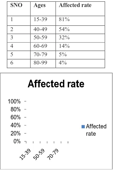
Table 1 Survival rate for men with brain tumor in England
Table 2- Survival rate for women with brain tumor in England
0% 20% 40% 60% 80% 100%
Affected rate
Affected rate
0% 20% 40% 60% 80% 100%
Affected rate
Affected rate
SNO Ages Affected Rate
1 15-39 77%
2 40-49 49%
3 50-59 30%
4 60-69 15%
5 70-79 7%
6 80-99 3%
SNO Ages Affected rate
1 15-39 81%
2 40-49 54%
3 50-59 32%
4 60-69 14%
5 70-79 5%
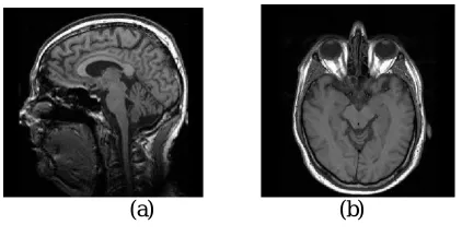
(a) (b)
Fig 1.1-weighted MR image
Fig1.a: This T1 weighted MR image Corpus of the brain shows cortex with white and grey matter, corpus callosum, lateral ventricle, thalamus, pons and cerebellum.
Fig1.b: This T1 weighted MR image of the brain shows eyeballs with optic nerve, medulla, vermis, and temporal lobes with hippocampus regions.
1.1 Overview of Hybrid Model
Fig 1.1 – Block structure of Hybrid Model registration
certain rules and gives corresponding weight to each group of pixel points according to similarity, finally the noise detected are filtering-treated. The weighted median filter is a variation of the median filter that incorporates spatial information of the pixels when computing the median value. A weighted median filter is implemented as follows:
W(x, y) =median {w1 × x1…wn × wn}
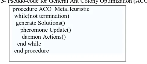
x1…..xn are the intensity values inside a window centered at (x,y)and w×n denotes replication of x, w times.Weighted median smoothers offer advantages over traditional linear finite impulse response (FIR) filters; it is shown in this paper that they lack the flexibility to adequately address a number of signal processing problems. In fact, weighted median smoothers are analogous to normalized FIR linear filters constrained to have only positive weights. The final Section represents the registration phase; here the hybrid model is implemented. This model consists of two methods non rigid and rigid method. In non rigid Method block based technique will be implemented using Ant colony optimization (ACO) for selecting optimal threshold value of the blocks from target image and normal image. The ant colony optimization algorithm (ACO) is a probabilistic technique for solving computational problems which can be reduced to finding good paths through graphs. Ant colony optimization algorithms have been applied to many combinatorial optimization problems, ranging from quadratic assignment to fold protein or routing vehicles and a lot of derived methods have been adapted to dynamic problems in real variables, stochastic problems, multi-targets and parallel implementations. It has also been used to produce near-optimal solutions to the travelling salesman problem. They have an advantage over simulated annealing and genetic algorithm approaches of similar problems when the graph may change dynamically; the ant colony algorithm can be run continuously and adapt to changes in real time. This is of interest in network routing and urban transportation systems. The following table consists of Pseudo-code for general ant colony optimization.
Table 3- Pseudo-code for General Ant Colony Optimization (ACO)
In rigid method the similarity measures are applied to unmatched blocks of non rigid method. The similarity measures the statistical dependence between images and it is most commonly used due to their accuracy, robustness and university. The similarity measures are 1.Sum of Squared Difference (SSD) 2. Contrast Checking (CC), 3.Average Intensity Difference 4. Correlation.
1.2 Related Works
Different approaches for automatic image registration have been proposed in medical imaging. This section describes different methods for MR brain image registration. Peter et al described a new high-dimensional non-rigid registration with two properties. Multi-modality and locality and he got best performance than previous method [10].Wilbert described automated application for the registration of MRI for Alzheimer patients with rigid-body transformation and non-rigid body” using classical match filter and (CMR) correlation filter and he found root-mean-squared (RMS) error through Match filter and correlation filter [16].Yeit et al specified automatic registration method for MR images using shape matching system with Gaussian model, this method successfully found necessary points fro register normal images and reference image[19].Thomas et al designed a new automatic and interactive methods for image registration for 3D MRI and SPECT Comparison for shows an accuracy[14].Wang et al described a Free-form deformations based on optimization used to speed up the registration process and avoid local minima.this performance evaluate with simulated images and real images [17]. Kovalev et al introduced a technique with Free-Form Deformation for non-rigid registration here Subdivision of NURBS is extended to 3D and is used in hierarchical optimization to speed up the registration and avoid local minima[8]. Peter et al described a new high-dimensional non-rigid registration with two properties. Multi-modality and locality and he got best performance than previous method [10].Wilbert explained comparison of registration methods for MRI brain images used nonlinear registration and warping models. it can get 31% more efficient than linear registration[16].
procedure ACO_MetaHeuristic while(not termination) generate Solutions() pheromone Update() daemon Actions() end while
Table 4: Overview of Registration methods
AUTHORS METHODS
Wang et al [17] Non-rigid registration using Free-Form Deformations, Non uniform Rational B Spline (NURBS)
Wilbert et al [18] Non-rigid registration Using Contium-Mechanics Warping Kovalev et al [8]
Xinhui et al [21] Hybrid optimization, similarity measure
Peter Roge lj et al [10] Non rigid registration multi-model Similarity measure
Alexis Roche et al [3] Intensity-based Similarity measure+ correlation Correlation ratio, mutual information
Yejt Han et al [19] Point matching with rigid registration + Gaussian model
Thomas P fluger et al [14] Interaction matching surface matching Uniformity index matching , woods Algorithm
Jorge Meyer et al [24] Histogram based Similarity measure with CT and MRI Dirk-Jan et al [6] Non-rigid fluid registration point Matching
Toyama et al [20] Semi-automatic method
Andre et al [2] 3D Voxel similarity based (VB) registration + Photo metric model parameters
Ceylan et al [4] Multiple sub Volume registration with multi modulation Polai man et al [11] Sum of square difference + Fast Fourier Transform
II. IMAGE ACQUISITION
The development of intra-operative imaging systems has contributed to improving the course of intracranial neurosurgical procedures. Among these systems, the 0.5T intra-operative magnetic resonance scanner of the Kovai Medical Center and Hospital (KMCH, Signa SP, GE Medical Systems) offers the possibility to acquire 256*256*58(0.86mm, 0.86mm, 2.5 mm) T1 weighted images with the fast spin echo protocol (TR=400,TE=16 ms, FOV=220*220 mm) in 3 minutes and 40 seconds. The quality of every 256*256 slice acquired intra-operatively is fairly similar to images acquired with a 1.5 T conventional scanner, but the major drawback of the intra-operative image is that the slice remains thick (2.5 mm). Images do not show significant distortion, but can suffer from artifacts due to different factors (surgical instruments, hand movement, radio frequency noise from bipolar coagulation). Recent advances in acquisition protocol [1] however make it possible to acquire images with very limited artifacts during the course of a neurosurgical procedure. The choice of the number and frequency of image acquisitions during the procedure remains an open problem. Indeed, there is a trade-off between acquiring more images for accurate guidance and not increasing the time for imaging.
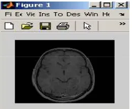
Images of a patient obtained by MRI scan is displayed as an array of pixels (a two dimensional unit based on the matrix size and the field of view) and stored in Mat lab 7.0.Here, grayscale or intensity images are displayed of default size 256 x 256.The following figure displayed a MRI brain image obtained in Mat lab 7.0.A grayscale image can be specified by giving a large matrix whose entries are numbers between 0 and 255, with 0 corresponding, say, to black, and 255 to white. A black and white image can also be specified by giving a large matrix with integer entries. The lowest entry corresponds to black, the highest to white. In routine, 21 male and female patients were examined. All patients with finding normal for age n=20 were included in this study. The age of patients ranged from 20 to 50 years. All the MRI examinations were performed on a 1.5 T magneto vision scanner (Germany).The brain MR images are stored in the database in JPEG format. The following figure shows the appearance of MR brain image in MAT LAB7.0.
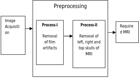
III. PREPROCESSING
Preprocessing functions involve those operations that are normally required prior to the main data analysis and extraction of information, and are generally grouped as radiometric or geometric corrections. Radiometric corrections include correcting the data for sensor irregularities and unwanted sensor or atmospheric noise, removal of non-brain voxels and converting the data so they accurately represent the reflected or emitted radiation measured by the sensor. In this hybrid model the preprocessing stage is divided in to two sections. First one for removal of film artifacts and second one for removal of unwanted portion of MRI.
Fig 3.1 -Block structure of Preprocessing Stage 3.1Removal of Film Artifacts
The MRI brain image consists of film artifacts or label on the MRI such as patient name, age and marks. film artifacts that are removed using tracking algorithm .Here, starting from the first row and first column, the intensity value of the pixels are analyzed and the threshold value of the film artifacts are found. The threshold value, greater than that of the threshold value is removed from MRI. The high intensity value of film artifacts are removed from MRI brain image. During the removal of film artifacts, the image consists of salt and pepper noise .The above image is given to enhancement stage for removing high intensity components and the above noise. The following figures explain the process of preprocessing stage.
Fig 3.2 - Removal of Artifacts from MRI
Table 5: Tracking Algorithm for Removal of film artifacts
3.2 Removal of Skull portions from MRI
The above table explains the algorithm for removal of film artifacts from MRI brain iamge.Second stage of preprocessing is removal of skull portion from MR brain images. This process is used to remove unwanted portion of MRI that means left, right and top skull portions that are not required for further processing.
Before Preprocessing After Preprocessing
Step 1: Read the MRI image and store it in a two dimensional matrix.
Step 2: Select the peak threshold value for removing white labels
Step 3: Set flag value to 255.
Step 4: Select pixels whose intensity value is equal to 255. Step 5:If the intensity value is 255 then, the flag value is set to zero and thus the labels are removed from MRI.
Step 6: Otherwise skip to the next pixel. Image
Acquisiti on
Preprocessing
Process-I
Removal of film artifacts
Process-II
Removal of left, right and
top skulls of MRI
Table 6: Tracking Algorithm for Removal of skull portions of MRI
Fig3.3 - Removal of left, right and top Skull portions of MRI
IV. ENHANCEMENT
Image enhancement methods inquire about how to improve the visual appearance of images from Magnetic Resonance Image (MRI), Computed Tomography (CT) scan; Positron Emission Tomography (PET) and the contrast enhancing brain volumes were linearly aligned. The enhancement actives are removal of noise, high frequency components, filtering the images. This part is use to enhances the smoothness towards piecewise-homogeneous region and reduces the edge-blurring effect. Conventional Enhancement techniques such as low pass filter, Median filter, Gabor Filter, Gaussian Filter, Prewitt edge-finding filter, Normalization Method are employable for this work. This proposed system describes the information of enhancement using weighted median filter for removing high frequency components such as impulsive noise, salt and pepper noise, etc.The following figure shows various filters applied during enhancement stage.
Fig 4.1 – Block Diagram for Enhancement Stage
Fig 3.3.
a-MRI with skull portion
Fig 3.3.b -MRI with Left skull portion removed
Fig 3.3.c -MRI with Right skull portion removed
Fig3.3.d -MRI with Top skull portion removed Step 1: Obtain the MRI image and store it in a two dimensional matrix.
Step 2: Start from left side first row, first column of the given matrix
Step 3: Select the peak threshold value from left side of the matrix.
Step 4: Assign flag value to 200.
Step 5: If the intensity value ranges from 200-255 then, the set the flag value to zero and thus the left skull
Portion of the MRI is removed.
Step 6: Repeat the above steps (2-5) to remove the right and
Enhancement
Median Filter
Weighted Median Filter
4. 1 Weighted Median filter
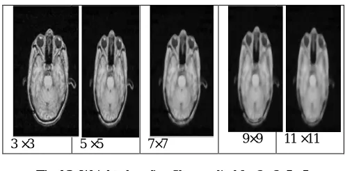
Fig 4.2: Weighted median filter applied for3 ×3, 5 ×5, 7 ×7, 9 ×9, 11 ×11 windows of MRI
The merit of using weighted median filter is, it can remove salt and pepper noise from MRI without disturbing of the edges. In this enhancement stage, the weighted median filtering is applied for each pixel of an 3 ×3, 5 ×5, 7 ×7, 9 ×9, 11 ×11window of neighborhood pixels are extracted and analyzed the mean gray value of foreground , mean value of background and contrast value. The following table explains the above features. In final 5 ×5 window of neighborhood pixels are extracted and implemented for removing high frequency components and noise from MRI.This procedure is done for all the pixels in the given MRI. The following expression is used for analyzing contrast of the corresponding windows.
Table 7: Performance Analysis of Weighted Median Filter
4.2 Median Filter
Median Filter can remove the noise, high frequency components from MRI without disturbing the edges and it is used to reduce’ salt and pepper’ noise.This technique calculates the median of the surrounding pixels to determine the new (denoised) value of the pixel. A median is calculated by sorting all pixel values by their size, then selecting the median value as the new value for the pixel. The amount of pixels which should be used to calculate the median. For each pixel, an 3*3, 5*5, 7*7, 9*9, 11*11 window of neighbourhood pixels are extracted and the median value is calculated for that window. The intensity value of the center pixel is replaced with the median value. This procedure is done for all the pixels in the image to smoothen the edges of MRI. High Resolution Image was obtained when using 3*3 than 5*5 and so on. The below example shows the model of median filter.
Example 1 shows the example of median filter with 3 x 3 windows
41,42,47,47 , 52, 55,55,64,66 median value
0.922 0.924 0.926 0.9280.93
3×3 5× 5 7×7 9 ×9 11 ×11
Contrast value
Contrast value
3 ×3 5 ×5 7×7 9×9 11 ×11
Pixel size
Mean gray
level of
foreground
Mean gray
level of Background
Contrast value
3×3
88.2121 3.3551 0.9267
5× 5
96.4823 3.6145 0.9278
7×7
95.9038 3.6561 0.9266
9 ×9
96.1042 3.7143 0.9256
11 ×11
96.1785 3.7485 0.9250
42 47 52
55 64 41
Table 8 Performance Analysis of Median Filter
The above 3×3, 5×5, 7×7, 9×9, 11×11 windows are analyzed in that 3×3 window is chosen based on the high contrast than 5×5, 7×7, 9×9, and 11×11.
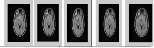
Fig 4.3: Median filter applied for3 ×3, 5 ×5, 7 ×7, 9 ×9, 11 ×11 windows of MRI
4.3Adaptive Filter
A new type of adaptive center filter is developed for impulsive noise reduction of an image without the degradation of an original image.
Fig 4.4: Adaptive filter applied for3 ×3, 5 ×5, 7 ×7, 9 ×9, 11×11 windows of MRI
0.911 0.912 0.913 0.914 0.915 0.916 0.917
3×3 7×7 11 ×11
Series1
Pixel size
Mean gray level of foreground
Mean gray level of Background
Contrast value
3×3 93.154 4.049 0.9167
5× 5 95.414 4.267 0.9144
7×7 95.475 4.305 0.9137
9 ×9 94.835 4.284 0.9136
C = (f-b) / (f + b)
Table 9 Performance Analysis of Median Filter
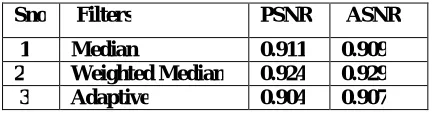
4.4 Performance Evaluation
It is very difficult to measure the improvement of the enhancement objectively. If the enhanced image can make observer perceive the region of interest better, then we can say that the original image has been improved. In order to compare different enhancement algorithms, it is better to design some methods for the evaluation of enhancement objectively. The statistical measurements such as variance or entropy can always measure the local contrast enhancement; however that show no consistency for the MRI. Three
Filtering techniques namely1) Median filter 2) Weighted Median filter 3) Adaptive filter were used for performance evaluation out of which Weighted Median filter proved to be best. The following table shows the Peak Signal-to-Noise Ratio (PSNR) and Average Signal-to-Noise Ratio (ASNR) values of the above filters.
CII = C Processed / C Original
C processed and C original = Contrasts of MRI
f = mean gray -level value of the foreground b= mean gray-level value of the background
Noise level= standard deviation ( σ ) of the background σ = √ (1/N) ∑i (bi-b) 2
bi = Gray level of a background region
N= total number of pixels in the surrounding background region (NB) PSNR = (p-b) / σ, ASNR =(f-b)/ σ
Table 10 Performance Analysis of filters
0.905 0.91 0.915 3 × 3 5 × 5 7 × 7 9 × 9 1 1 × 1 1
Contrast value
Contrast valuePixel size Mean gray level of foreground Mean gray level of Background Contrast value 3×3
92.5059 4.2789 0.9116
5× 5
95.1252 4.5236 0.9092
7×7
95.2662 4.5717 0.9084
9 ×9
94.1861 4.5462 0.9079
11 ×11
92.5125 4.4779 0.9077
Sno Filters PSNR ASNR
1 Median 0.911 0.909
2 Weighted Median 0.924 0.929
Table 11: Tracking Algorithm for Weighted Median filter
V. MRI BRAIN IMAGE REGISTRATION
Image Registration is a basic task in image processing used to match two or more images taken at different sensors of from different view points. Image registration algorithms can also be classified according to the transformation model used to relate the reference image space with the target image space. The first broad category of transformation models includes linear transformations, which are a combination of translation, rotation, global scaling and shear components. Linear transformations are global in nature, thus not being able to model local deformations. The second category includes 'elastic' or 'non-rigid' transformations. These transformations allow local warping of image features, thus providing
support for local deformations. Non rigid transformation approaches include polynomial warping, interpolation of smooth basis functions.In another category of image registration is the process of aligning images from a single modality or from different modalities. In this hybrid model, we described single modality because MR Brain Images are acquired by the same 1.5T scanner and same sensor type. This method has two processes simultaneously. First one is rigid method (linear transformation), next one is a non-rigid method (non-linear transformation). In rigid method based on the following similarity measures, such as Contrast difference (CD), Sum of square difference (SSD), Ratio image uniformity. The following figure displays that the classification of image registration.
Fig 5.1 – Classification of Image Registration
0.89 0.9 0.91 0.92 0.93 0.94
PSNR ASNR
Step 1: Read the MR image and store it in a two dimensional matrix
Step 2: Extract matrix of size 3 ×3 from the given image and apply weighted median filtering
Step 3 : Intensity values of 3 ×3 matrix are compared with the given range of values.
If the intensity value is less than 50, a weight 0.1 is multiplied with the intensity value
Else If the intensity value ranges from 51-100, a weight 0.2 is multiplied with the intensity value.
Else If the intensity value ranges from 101-150, a weight 0.3 is multiplied with the intensity value
Step 4: Calculate median value for the above 3 ×3 matrix Step 5: Replace the center intensity value of the 3 ×3 matrix by the median value that was calculated Step 6: Repeat the above steps (step 2 to 5) for the matrices of size 5 ×5, 7 ×7, 9 ×9 and 11×11.
Registration
(Transformation model)
Non linear Transformation
(Non- rigid) Linear transformation
5.1 Non Rigid Registration
Now the focus of medical image registration has shifted to non-rigid registration. It is also a core component in computational neuroanatomy. Non rigid registration is the general term for an algorithm for the alignment of data sets that are mismatched in a nonlinear or non uniform manner. The term ''matching'' is used to refer to any process that determines correspondences between data sets. Non-rigid registration has traditionally used physical models like elasticity and fluids. These models are very seldom valid models of the difference between the registered images; this paper presents a non-rigid algorithm for registering normal image and target image. This paper consists of an efficient registration framework which has features of block based technique. Here normal patient image is compared with reference images. The following table shows normal image and reference image taken for comparison.
Fig 5.2- The Sample reference image and normal image
Fig 5.3: Flow chart for Non- rigid Registration
5.1.1 Block Based Method
In Block based technique, both the given reference MR brain image (256 × 265) and the normal image (256 × 265) has been divided into several blocks. Each and every block of both the images is 64 ×64. After blocking, subtraction has been done between the two images. This subtracted value is then checked with the threshold value, in our method. Then first block from both the images were subtracted and the average value of all the pixels in that block were calculated. This average value is then compared our threshold value of 80,000 and if any of which is found to cross this limit, those patient details will be stored in the database as a doubtful case.
Fig 5.4 – Flow diagram of Block based technique
Average Intensity Measure
Average intensity measure for blocks of both normal and target image was calculated and compared. If there is any abnormality found in the normal image then it is stored in segmented database. Otherwise it is stored in normal database. In the following table, block 1 to block 4 of both source and target image does not have difference in average intensity but in block5 to block 8 has different values. Those values are stored in segmented database.
Table 12: Average intensity value based on blocks
Image Block 1
Block 2
Block 3
Block 4
Block 5
Source 31 67 51 2 68
target 1 31 67 51 2 77
target 2 31 67 51 2 68
target 3 31 67 51 2 68
Image Block 6
Block 7
Block 8
Block 9
Block 10
Source 71 86 5 49 87
target 1 91 86 5 57 97
target 2 71 86 5 75 105
target 3 101 91 5 49 90
Image Bloc k 11
Bloc k 12
Bloc k 13
Bloc k 14
Bloc k 15
Blo ck 16
Source 62 4 8 38 14 2
target
1 62 4 8 38 14 2
target
2 62 4 8 38 14 2
target
3 62 4 8 38 14 2
Segmented Image Database
5.2 Rigid Registration
Rigid body registration is one of the simplest forms of image registration. The shape of a human brain changes very little with head movement, so rigid body transformations can be used to model different head positions of the same subject. Registration methods described in this chapter include within modality, or between different modalities such as PET and MRI. Matching of two images is performed by finding the rotations and translations that optimize some mutual function of the images. Within modality registration generally involves matching the images by minimizing the sum of squared difference between them. For between modality registrations, the matching criterion needs to be more complex. For rigid body registration, rotations and translations are adjusted. The changes could arise for a number of different reasons, but most are related to pathology. Because the scans are of the same subject, the first step for this kind of analysis involves registering the images together by a rigid body transformation. This rigid method consists of the following similarity measures, such as Contrast difference, Sum of square difference,Correlation using point, similarity measure .An application of rigid registration is the field of morphometry, and involves Identifying shape changes within single subjects by subtracting coregistered images acquired at Different times.
5.2.1 Similarity Measure
Image similarities are broadly used in medical imaging. An image similarity measure quantifies the degree of similarity between intensity patterns in two images. The choice of an image similarity measure depends on the modality of the images to be registered. In this section ,similarity measures are applied to patient or normal images and reference images. The merit of this implementation gives sum of square intensity difference (SSD) and contrast checking between both the images. We have developed a similarity with three references of tumor image and normal images from patient database. The following table consists of one normal image and three reference image, it consists of tumor tissue.
5.2.1.1 Contrast checking
Contrast checking is one of the methods in similarity measure. Contrast for the reference images and normal image is computed based on average background and average foreground value of MRI. Contrast checking for a given image is calculated by the given formula.
C = (f-b) / (f + b)
C = Contrast of the given image
f = mean gray -level value of the foreground b= mean gray-level value of the background
The below table shows the contrast value for the given images.
Table 13: Image Contrast Analysis
5.2.1.2 Sum of Squared Difference (SSD)
Sum of Squared Differences (SSD) is one of the simplest of the similarity measures which is calculated by subtracting pixels within a square neighborhood between the reference image I1 and the target image I2 followed by the aggregation of squared differences within the square window, and optimization. In this section, the sum of squared difference (SSD) is applied for each pixel of an 3 ×3, 5 ×5, 7 ×7, 9 ×9, 11 ×11window of neighborhood pixels in target image and reference image. The average value of SSD is found for both the images. Sum of square difference is given by :
SSD= Sum of square of pixels / Total number of pixels in the given window
Image name
Contrast Avg-Back Ground
Avg- Fore ground
Table 14: Sum of squared difference of Normal image and tumor image
The above figure describes the sum of square intensity difference of target images is higher than normal image
5.2.1.3 White cells calculation
Fig 5.5: Number of white pixels in Normal and reference Images
2500300035004000 Normal
Tumor 1 Tumor 2 Tumor 3
Average of SSD
Average of SSD
0 500 1000 1500
A
xi
s
Ti
tl
e
No of white pixels
No of white pixels
Image name
Sum of square Difference (SSD)
Average of SSD
Normal 195139692
2977.595398 Tumor 1 232541734
3548.305267 Tumor 2 230918327
3523.534042 Tumor 3 224479823
3425.290268
Image name No of white pixels
Normal 418
Tumor 1 594
Tumor 2 1113
Table 15: Algorithm for Rigid registration
5.2.1.4 Point Mapping
Point mapping is the basic statistical approach to registration and it is a match metric technique it gives a measure of the degree of similarity between an image and a template. Point similarity measures can be derived from global measures and enable detailed relative comparison of local image correspondence. For performing Image Registration, We have to get the enhanced image in the same size as that of the original image (image without tumor). Here, we have taken two reference points first, in front view and second in the top view of the image.
Fig 5.6: Using point similarity measure in MRI
Fig 5.7: Before Correlation
The enhanced image has to be resized to the original image size by fixing the same reference points as in the original image. Since in our technique, the size of the original image is 256*256, the enhanced image has been resized to (256-x)*(256-y) by removing the extra portions in the image.
Fig 5.8 - After Correlation Step 1: Read the image obtained from non rigid registration
Step 2: Apply similarity measures for the above image (i) Find contrast of those images using Average foreground and background value c= (f-b)/(f+b)
(ii) Calculate Sum of square difference (SSD) using SSD=Sum of square for pixels/ Total number of pixels in the window of size 3 ×3 , 5× 5, 7×7 , 9×9 and 11×11 (iii) Analyze the average Sum of squared difference of those images
VI. CONCLUSION
This paper proposed a hybrid model for MR brain image registration using transform model like rigid method (linear Transformation) and non-rigid method (non- linear transformation). Initially, MR brain image is acquired. Secondly the film artifacts and unwanted portions of brain are removed using tracking algorithms and the image is assigned as a new image. With this new image the weighted median filtering is applied to remove high frequency components. Finally the MR images are entered in to registration. Here, the reference (tumor) and normal image (patient) are involved to rigid method and non rigid method. In non rigid method the block based technique is implemented. The reference image and normal images are split as several blocks of size 64 ×64. Intensity pair of each block of those images is compared. If any changes occur in those blocks then it will be assigned as a new image and it is given to the next stage. In rigid method, the intensity pattern of both the images are analyzed using similarity measures like contrast checking (CC), Sum of Squared Difference (SSD) and measurement of T1 weighted image. The merit of the hybrid model is very simple because MR images are registered using similarity measures with block based technique. The above methods produce accurate result than previous methods and it produces the same output every time and one of the demerits of this proposed hybrid model is that it will work only for the MR images with the dimension 256 ×256. This method does not accept CT or PET brain images.
REFERENCES
1. Alexandra Flowers MD, “Brain Tumors in the Older Person “, November/December 2000, Vol. 7, No.6. (1)
2. André Collignon, Dirk Vandermeulen, Paul Suetens,Guy Marchal,” 3D multi-modality medical image registration using feature space clustering “,SpringerLink, Volume 905/1995, Berlin 1995.(2)
3. Alexis Roche, Gregoire Malandain, Nicholas Ayache, Sylvain prima, “Towards a better comprehension Medical Image Registration”, Medical Image Computing and Computer-Assisted Intervention-MICCAI’99, PP555-566, 1999.(3)
4. Ceylan.C, Van der Heide U.A, Bol G.H, Lagendijk .J.J.W,Kotte A.N.T.J,”Assessment of rigid multi-modality image registration consistency using the multiple subvolume registration(MSR) method”,Physics in Medicine Biology,50N101-n108,2005.(4)
5. Darryl de cunha, Leila Eadie, Benjamin Adams, David Hawkes, “Medical Ultrasound Image similarity measurement by human visual system(HVS) Modelling”, spingerlink, volume 2525, January, berlin, 2002.(5)
6. Dirk-Jan Kroon,” Multimodality non-rigid demon algorithm image registration “,Robust Non-Rigid Point Matching, 16 Sep 2008 .(6)
7. Joerg Meyer,” Histogram Transformation for Inter-Modality Image Registration”,Biomedical Engineering Department, Irvine.(24)
8. John Ashburner , Karl J. Friston,” Rigid body registration “, The welcome dept of image neuro science , 12 queen square, London.(7)
9. Konstantinos G. Denpanis,”Relationship Between the Sum of Squared Difference(SSD) and Cross Correlation for Template Matching”, York University , Version 1.0, Dec 23,2005.(8)
10. Kovalev, V.A, Kruggel, F, Gertz, H.-J, von Cramon, D.Y.,” Three-dimensional texture analysis of MRI brain datasets”, Medical Imaging, IEEE Transactions on Texture analysis, Volume 20, Issue 5, May 2001. (9)
11. Krzysztof Wrobel, Piotr Porwik,”Comparative Investigations of similarity measure exploited in medical images preselection”, Journal of medical informatics & Technologies, Volume 8,2004.(26)
12. Leonid Teverovskiy, Owen Carmichael, Howard Aizenstein,Nicole Lazer, Yanxi Liu,” Feature based Vs intensity-based brain image registration: Voxel level and structure level performance evaluation”, School of Computer Science Carnegie Mellon University, Nov 2006.(10)
13. Panos kotsas,” Non-rigid Registration of medical images using an Automated method”,World academy of science, Engineering and Technology , 2005.(11)
14. Peter Rogeli, Stanislav, Kovacic, James C.Gee, “ Point similarity measures for non-rigid registration of multi-model data source”, Elsevier Science Inc, volume 92, issue1, October, USA 2003.(12)
15. Peter J. Kostelec, Senthil Periaswamy,” Image Registration for MRI,” Modern Signal Processing, MSRI Publications,V olume 46,2003.(25)
16. Po Lai-Man, Kai Guo,” Simple noncircular correlation method for exhaustive sum square difference matching”,Society of photo-optimal instrumentation engineering,Vol 46, issue 10,2007.(13)
17. Survival Rate for Brain tumor and Cancer Society, Cancer Facts and Figures, American Cancer Society, US 2004.(14)
18. Survival Rate for Brain tumor and Cancer, Canadian Cancer Statistics, National Cancer Institute of Canada, 2004.(15)
19. Thomas Pfluger, Christian Vollmar, Axel Wismuller, Stefan Dresel, Frank Berger, Patrick Suntheim,Gerda Leinsinger,Klaus Hahn,”Quantitative Comparisonof Automatic and Interactive Methods for MRI-SPECT image Registration of the Brain based on 3-Dimensional calculation of error”,The journal of Nuclear Medicine, Vol 41, No 11 1823-1829,2000.(16).
20. Tsutomu Soma, Akihiro Takaki, Satomi Teraoka, Yasushi Ishikawa, Kenya Murase, Kiyoshi Koizumi,” Behaviors of cost functions in image registration between Tl brain tumor single-photon emission computed tomography and magnetic resonance images “,Annals of Nuclear Medicine, SpringerLink, Volume 22, Number 9 / November, 2008.(17)
21. Wilbert Mcclary, “Comparision of Methods of Registration for MRI Brain images”, Engineering Research and technology Report, 925, PP423-4153.(18)
22. Wang J., Jiang T. "Nonrigid registration of brain MRI using NURBS" Pattern Recognition Letters 28(2): 214-223, 2007.(19)
23. Wilbert McClay,” Comparison of Methods of Registration for MRI Brain Images”,Engineering Research and Technology Report. (20)
24. Yeit Han, Hyun Wook park,”Automatic brain MR images registration based on Talairach reference system”,Proceedings of international conference on image processing(ICIP),volume:1,ISSN : 1522-4880,sep 2003.(21)
25. Yubei Shimada, Koji Uemura Babak A. Ardekani, Tsukasa Nagaoka, Kiichi Ishiwata, Hinako Toyama, Kenichirou Ono, Michio Senda,” Application of PET-MRI registration techniques to cat brain imaging “,Journal of Neuroscience Methods, Volume 101, Issue 1, 15, Pages 1-7 ,August 2000.(22)