K. R. Kavanagh, C. T. Kelley
North Carolina State University, Center for Research in Scientific Computation and Department of Mathematics, Box 8205, Raleigh, N. C. 27695-8205, USA
([email protected], Tim [email protected]).
C. T. Miller
Center for the Advanced Study of the Environment, Department of Environmental Sciences and Engineering, University of North Carolina, Chapel Hill, North Carolina 27599-7431, USA (casey [email protected]).
C. E. Kees, R. M. Darwin, J. P. Reese
North Carolina State University, Center for Research in Scientific Computation and Department of Mathematics, Box 8205, Raleigh, N. C. 27695-8205, USA
(chris [email protected], [email protected],[email protected]).
M. W. Farthing
Center for the Advanced Study of the Environment, Department of Environmental Sciences and Engineering, University of North Carolina, Chapel Hill, North Carolina 27599-7431, USA (matthew [email protected]).
M. S. C. Reed
North Carolina Supercomputing Center 3021 Cornwallis Rd. Research Triangle Park, NC 27709, USA ([email protected]).
Abstract. Problems involving the management of groundwater resources occur routinely,
and management decisions based upon optimization approaches offer the potential to save substantial amounts of money. However, this class of application is notoriously difficult to solve due to non-convex objective functions with multiple local minima and both nonlinear models and nonlinear constraints. We solve a subset of community test problems from this ap-plication field using MODFLOW, a standard groundwater flow model, and IFFCO, an implicit filtering algorithm that was designed to solve problems similar to those of focus in this work. While sampling methods have received only scant attention in the groundwater optimization literature, we show encouraging results that suggest they are deserving of more widespread consideration for this class of problems. In keeping with our objectives for the community problems, we have packaged the approaches used in this work to facilitate additional work on these problems by others and the application of implicit filtering to other problems in this field. We provide the data for our formulation and solution on the web.
Keywords: Implicit filtering, Well field design, Groundwater flow and transport
1. Introduction
a usable quality at a minimum cost. Accomplishing these goals requires a model to describe the system of concern, an appropriate objective function, constraints, and an optimization algorithm. The objective function and con-straints provide the linkage between the simulation model and the optimizer. Because porous media systems are typically heterogeneous over small scales and described by nonlinear processes, subsurface simulators can be expensive to evaluate and subject to uncertainty, or stochastic in nature. The resulting optimization problems can also be difficult, with objective functions that are non-convex and have multiple local minima, and both models and constraints that are nonlinear. For these reasons, subsurface optimization problems are both important and challenging.
To aid the evolution of optimal design of subsurface flow and transport applications, a set of community problems (CP’s) was developed, [30], that are typical of problems commonly encountered and which cover a range of complexity. It was reasoned that focusing on a common set of CP’s would allow for not only advancement of approaches to solve an important set of problems, but also a means to aid comparison of various aspects of the so-lution approach on the same set of problems. It was also anticipated that the CP’s would catalyze the introduction of new classes of optimization methods into the groundwater field and result in more active participation of the ap-plied mathematics community in the evolution of solution approaches for this class of application.
A subset of the CP’s is a standard water supply application. Roughly speaking, the objective is to locate a set of water supply production wells and find their pumping rates such that cost is minimized subject to constraints on the total amount of water that must be produced, the hydraulic head in the wells, the production capacity of a well, and the portion of the domain over which a well may be located. Evaluation of the objective function requires a groundwater flow simulator that solves for hydraulic head as a function of space and time given a spatial and temporal domain, material properties, auxiliary conditions, and well design information.
In this paper we take the view that there is enough structure in the problem to use a deterministic sampling method. These methods are designed to solve problems with difficult, but not violently oscillatory optimization landscapes, such as the ones in Figures 8, 9, 10, 11 in§ 8. Gradient-based methods are likely to have trouble with such problems, either finding local minima, stag-nating, or failing to find a descent direction. In our testing of a gradient-based method, which we report in§8, we observed this type of failure. The Nelder-Mead [34], Hooke-Jeeves [23], MDS [16, 43], DIRECT [25], and implicit filtering [21, 20, 26] are examples of discrete sampling methods.
The objectives of this work are: (1) to provide an initial analysis of a subset of groundwater CP’s, which have been recently published; (2) to formulate a solution to these problems with a sampling method, in this case implicit filtering; (3) to compare the results with a genetic algorithm approach, and to explain why traditional gradient-based methods can and do fail; (4) to examine the characteristics of the solution space and illustrate the challenges that this class of problem poses; and (5) to point the way toward future improvements for the solution of this class of problem.
2. Conceptual Model
An aquifer is a fully saturated, water-bearing region and is considered con-fined if bounded on both the top and the bottom by essentially impermeable material. An unconfined aquifer has the water table as its upper bound. The main difference between the two geological formations is that the saturated thickness of an unconfined aquifer varies as the hydraulic head varies, thus leading to a nonlinear free-boundary problem.
We consider a well-field design problem. The hydrological settings are homogeneous confined and unconfined aquifers in three spatial dimensions. For the problems considered, a set of wells is distributed in the domain. Each well is allowed either to inject or extract water. Well-field design problems involve the selection of well locations and pumping rates to minimize the cost of water production. The cost of supplying water typically involves the cost to drill, equip, and connect wells to a treatment or distribution system, and the cost to pump the water and maintain the well. In turn, the cost to pump groundwater depends upon the energy needed to lift the water from its level below the ground surface to the discharge point and to supply sufficient discharge pressure to achieve the desired flow.
flow rate is realistic. This is because any transients decay very early in the five year time horizon.
3. Formulation
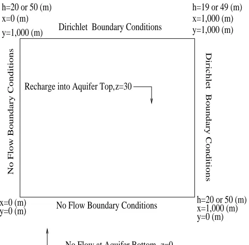
The physical domain, see Figure 1, isΩ = [0,1000]×[0,1000]×[0,30]m with the ground elevation atzgs = 60m for the confined aquifer andzgs = 30
m for the unconfined aquifer.
Flow in saturated porous media can be described, [30], by
Ss
∂h
∂t =∇ ·(K∇h) +S, (1)
whereSs (1/m) is the specific storage coefficient, the unknownh(m) is the
hydraulic head, K (m/s) is the hydraulic conductivity [30]. Here the source termS is a model of the wells, a sum ofδ-functions that satisfies
Z
Ω
S(t)dΩ =
n
X
i=1
Qi. (2)
Ωis the spatial domain. The wells are assumed to extract from near the bottom of the aquifer. If a numerical solution is discrete in thez-dimension then only the bottom layer of cells/elements should include the well source terms.
For the confined aquifer, we use the following boundary and initial condi-tions: ∂h ∂x x =0 = ∂h ∂y y=0 = ∂h ∂z z =0
= 0, t >0 (3)
qz(x, y,30, t >0) =−1.903×10⁻⁸(m/s) (4)
h(1000, y, z, t >0) = 50−0.001y(m) (5)
h(x,1000, z, t >0) = 50−0.001x(m) (6)
h(x, y, z,0) =hs (7)
Here
qz=−K
∂h ∂z
flow problem prior to the addition of wells. We useSs= 10−6(1/m). For the
unconfined aquifer, (4), (5) and (6) are replaced with
qz(x, y, h, t >0) =−1.903×10⁻⁸(m/s), (8)
h(1000, y, z, t >0) = 20−0.001y(m), (9) and
h(x,1000, z, t >0) = 20−0.001x(m). (10) Ss = 2.0 ×10⁻¹ is the specific yield of the unconfined aquifer. For the
homogeneous applications,K = 5.01×10⁻⁵
(m/s).
Dirichlet Boundary Conditions
Dirichlet Boundary Conditions
No Flow Boundary Conditions
No Flow Boundary Conditions
x=0 (m)
z=0 h=20 or 50 (m)
y=1,000 (m)
x=0 (m) y=0 (m)
h=19 or 49 (m) x=1,000 (m) y=1,000 (m)
h=20 or 50 (m) x=1,000 (m) y=0 (m) z=30
Recharge into Aquifer Top,
No Flow at Aquifer Bottom, Figure 1. Physical Domain
4. Objective Function
We consider a capital costfcand an operational costfoseeking to minimize
fT =fc+fo.The objective function depends on the pumping rates{Q i}ni=1 and locations{(xi, yi)}in=1ofnoperating wells. Note thatQi<0means the
well is extracting water, and Qi > 0means the well is injecting water. For
Since there is a fixed installation cost for wells, an important aspect of the optimization procedure is the manner in which wells are removed from the design, thereby significantly decreasing the total cost. A well is considered installed and operating if |Qi| > 0.0001. If the optimizer specifies a value
with |Qi| ≤ 0.0001 then we neither apply the well source term nor do we
include the cost of the well in the objective function. This approach results in non-smoothness in the objective function, but provides a reasonable mecha-nism for removing wells from the design that our optimizer was capable of triggering.
The objective function is given by
fT =
n
X
i=1
c0dbi0+
X
Qi<−.0001
c1|Qmi |b1(zgs−hmin)b2
| {z }
fc
+ (11)
tf
X
i,Qi<−.0001
c2Qi(hi−zgs) +
X
i,Qi>.0001
c3Qi
| {z }
fo
,
where the cost coefficients cj and exponentsbj are given in Table I. Heredi
is the depth of well i,Qm
i is the design pumping rate,hmin is the minimum
allowable head,hiis the hydraulic head in welli,tf is the total design time,
which was taken as 5 years, and zgs is the elevation of the ground surface.
Injection wells are assumed to operate under gravity feed. Infc, the first term
denotes the cost to install all the wells, and the second term accounts for the additional cost for pumps for the extraction wells. In fo we have a lift cost
that applies to the extraction wells and an injection cost that applies to the injection wells.
The design pumping rates{Qm
i }, i.e. the maximum rates at which a given
well can pump, depend upon the aquifer properties, casing and discharge piping size, pump characteristics, screen length and opening size, effective-ness of the development, and local geochemical conditions. One could, in principal, treat the properties of the wells and pumps as optimization param-eters. We do not do this here, and focus on more fundamental aspects of the formulation.
5. Constraints
Table I. Objective Function Data
data value units
c0 5.5×10 3
$/mb
c1 5.75×10 3
$/[(m3
/s)b1
·mb2]
c2 2.90×10− 4
$/m4
c3 1.45×10− 4
$/m3
b0 0.3
-b1 0.45
-b2 0.64
-zgs 60 confined m
zgs 30 unconfined m
di zgs m
Qm
i 1.5Qi m
3
/s
QT = n
X
i=1
Qi ≤QminT , (12)
Qemax≤Qi ≤Qimax, i= 1, ..., n, (13)
and
hmin≤hi ≤hmax, i= 1, ..., n, (14)
where QT is the net pumping rate, QminT is minimum allowable total
ex-traction rate, Qemax is the maximum extraction rate at any well, Qimax is the maximum injection rate at any well, hmax is the maximum allowable
head, andhminis the minimum allowable head. Values for the bounds in the constraints are given in Table II. We require that the wells be at least 200 m from the boundary on which Dirichlet boundary conditions are applied, i. e.
0≤xi, yi ≤800. (15)
In addition to (15), we do not allow two wells to occupy the same grid point. In the course of the optimization, if two wells converge to the same location, our choice of simulator would implement the two wells as one well, operating at the sum of the two pumping rates. In turn, only one well would operate in the flow simulation, yet two wells would be included in the instal-lation cost. For our choice of spatial discretization, this indirectly implies that the distance between wells is at least 20m apart.
more that the operating costs for a single year. Therefore, once the minimum extraction target is reached, it would only make sense to drill additional wells if the long-term operating savings is significant. Since five wells extracting at the maximum level satisfy (12) with equality, one logical formulation of the problem is to find the optimal location of five wells, each extracting as much as possible.
Constraint (13) reflects physical limits on the pumps and well design. Well designs are typically limited by the size distribution of the porous medium and the resulting size of the well screen.
The upper bound in constraint (14) keeps the hydraulic head below the surface elevation and the lower bound ensures that excessive drawdown will not occur. This constraint is a linear function of the pumping rates for the confined case but a nonlinear function for the unconfined case, and in both cases a highly nonlinear function of the locations of the wells.
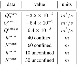
Table II. Constraint Data
data value units
Qmin
T −3.2×10−
2
m3
/s Qemax −6.4×10⁻³ m3/s
Qimax 6.4×10⁻³ m3/s
hmin
40 confined m hmax
60 confined m hmin 10 unconfined m
hmax
30 unconfined m
5.1. OPTIMIZATION PROBLEMFORMULATION
In this section we describe how we packaged the problem for the optimization algorithm. The objective function fT is discontinuous, and some of the
con-straints (13) and (15) are simple bounds on the variables. Implicit filtering, the optimization method we use in this paper, is designed to handle difficult objective functions and bound constraints.
If we set n = 5, then the constraints (12) and (13) require the pumping rates to be exactly Qmin
T /5. Thus, in this situation, we need only optimize
when either (12) or (14) are violated. Our implementation of implicit filtering will assign an artificial (see § 6.2) value to the function when it returns a failure. This is a standard approach for handling nonlinear constraints in many sampling methods, [42, 9, 27].
We will fix the number of wells and consider the vector of design variables
Z = (x1, . . . , xn, y1, . . . , yn, Q1, . . . , Qn)T ∈R3n.
We define the feasible set for the bound constraints as
D0={Z| (13) and (15) hold.}={Z|Zimin≤Zi≤Zimax}. (16)
Our optimization problem is
min
Z∈D0
fT(Z), (17)
wherefT is given by (11) if (12) and (14) are satisfied and a failure is reported
if either of (12) or (14) are violated.
6. Implicit Filtering
The objective function is highly nonlinear and non-convex, discontinuous because of the jumps as wells are added and deleted, and noisy, because of internal iterations in the simulators. For these reasons, as we said in § 1, a conventional gradient-based optimization method may fail. A sampling method, which only evaluates the objecive function and constraints to guide the optimization, is most appropriate for this kind of problem.
In this paper we use IFFCO [10], a FORTRAN implementation of the implicit filtering algorithm [26, 21, 20]. We based this decision on our own familiarity with the optimizer and our past success with it on other problems of a similar mathematical nature [4, 42, 9], although we are not aware of any use of implicit filtering for the type of application problem of concern in this work. This choice significantly influenced the decisions on handling constraints and the locations of the wells.
6.1. THE ALGORITHM
Implicit filtering is a projected quasi-Newton method that uses finite dif-ference gradients. The difdif-ference increment is reduced as the optimization progresses, thereby avoiding some local minima, discontinuities, or nons-mooth regions that would trap a conventional gradient-based method. The problems considered in this paper are exactly the kind that the method was designed to solve.
Implicit filtering begins by rescaling the variables so that the feasible region is
D={ξ|0≤ξi≤1}. (18)
We will discuss the algorithm in terms of the scaled feasible region in (18) but the application in terms of the actual bounds (16).
To make the transition fromfT to the scaled form, we defineξ
component-wise by
ξi = (Zi−Zimin)/(Zimax−Zimin)
and let
f(ξ) =fT(Z). The optimization problem forf is now
minξ∈Df(ξ).
For a given difference increment (called a scale)δ ∈(0,1/2]andξ∈ D, we let∇δf(ξ)be the difference gradient whose components are
− the central difference gradient in theith coordinate direction if both of ξ±δei ∈ D, or
− the one-sided difference gradient in theicoordinate direction if only one ofξ±δei ∈ D.
Since δ ≤ 1/2, at least one of ξ ±δei ∈ D. We let the stencil S(ξ) be
those points in the centered difference stencil that are in Dand used in the computation of∇δf. If
f(ξ)≤ min
η∈S(ξ)f(η) (19)
we say that stencil failure has occurred and terminate the quasi-Newton iteration at that scale.
If H is a model Hessian, a projected quasi-Newton iteration from ξ has the general form
whereP is the projection ontoD
P(ξ)i =
0 ifξi ≤0
ξi if0< ξi <1
1 ifξi ≥1
In IFFCO, the step lengthλis computed with a quadratic model [10] and a step is accepted if the sufficient decrease condition
f(ξ(λ))−f(ξ)≤α∇δf(ξ)T(ξ(λ)−ξ), (20)
holds. In IFFCO, as is standard, α = 10−4. We say that the quasi-Newton iteration is successful if
kξ−ξ(1)k ≤τ δ. (21)
The algorithmic parameterτ can have a significant effect on the performance of the optimization. For the problems we consider here, however, we were able to successfully use the default value ofτ = 1.
The finite difference projected quasi-Newton loop in IFFCO is summa-rized in algorithm fdquasi. fdquasi is a naturally parallel algorithm; all the function evaluations needed to compute∇δf can be done in parallel. We
exploited this simple parallelism to perform the computations reported in this paper.
Algorithm 1 fdquasi(ξ, f, pmax, τ, δ, amax) p= 1
whilep≤pmaxandkξ− P(ξ− ∇δf(ξ))k ≥τ δdo
computef and∇δf
if (19) holds then
terminate and report stencil failure
end if
update the model HessianHif appropriate; solveHd=−∇δf(ξ)
use a backtracking line search, with at mostamaxbacktracks, to find a step lengthλ
ifamaxbacktracks have been taken then terminate and report line search failure
end if
ξ ← P(ξ+λd) p←p+ 1 end while
ifp > pmaxreport iteration count failure
Implicit filtering calls fdquasi repeatedly with a sequence of scales{δk}.
Algorithm 2 imfilter(ξ, f, pmax, τ,{δk}, amax)
fork = 0, . . .do
fdquasi(ξ, f, pmax, τ, δk, amax)
end for
The algorithmic parameters that are important to implicit filtering are the limitamaxon the number of step size reductions, pmaxon the number of nonlinear iterations, and the parameterτ in the termination criterion. For the calculations reported here, we set pmax = 100 (the default), τ = 1 (the default), andamax= 3(the default). The parameters in imfilter that control the quasi-Newton loop are the sequence of scales {δk}. Our choice in this
work was
δk = 2−k−1, 0≤k≤10.
The analysis of implicit filtering begins with the paradigm
f =fS+φ (22)
wherefS is a smooth function andφrepresents the “noise” in the problem.
For the theoretical convergence results in [42, 26, 11] we assume thatφis an everywhere-defined function onΩand set
kφkS(ξ)= max
η∈S(ξ)|φ(ξ)|. One can show that if either (19) or (21) hold, that
kP(ξ− ∇fS(ξ))k=O(δ+kφkS(ξ)/δ). (23) The convergence theory for implicit filtering [26, 21, 11] are based on (23).
IFFCO supports the SR1 [7, 18] and the BFGS [41, 8, 19, 22] quasi-Newton models of the Hessian. We used the SR1 update in this paper. In our experience the SR1 update performs better for bound-constrained problems.
Implicit filtering can be restarted after it terminates and the convergence theory [21] is stronger if one does that. In practice, restarting usually has no effect. For the problems in this paper, however, we had to restart IFFCO once to obtain consistently good results.
6.2. FAILURE OF THE FUNCTION
IFFCO responds to a failure offin two ways. If the failed function evaluation fT(z)is part of the evaluation of∇hfT(ξ), then an artificial value [9] of
is assigned tof(z). Heref∗
is the largest function value in the stencilS(ξ). If the function evaluation failure is part of the line search, the the value f scale is assigned tofT.
f scaleis an approximation to the maximum value of fT in the feasible set D0 for the bound constraints (16). We setf scaleto 20% more than the value off at the initial iterate in this paper.
This approach to handling constraints is natural if the failure of the objec-tive function is a consequence of, for example, an internal iteration’s failure to converge. In the case of the problem considered here, while the constraints are directly specified by (14), the evaluation ofhirequires a call to the simulator
which, as a function of the well locations, is highly nonlinear even for the continuous problem. For the discrete problem considered here, where the well locations are rounded to grid points before the call to the simulator, the constraint function is discontinuous.
7. Evaluation of the Objective Function
IFFCO requires an external subroutine to evaluate the objective functionfT.
To do this we must compute the hydraulic head values, {hi}, at the well
locations {(xi, yi)}for a given set of pumping rates {Qi}. Computation of {hi}uses a groundwater flow simulator to solve (1). For this work we use the
U.S. Geological Survey code MODFLOW-96 [31]. MODFLOW is a block-centered finite difference code that simulates saturated groundwater flow and allows for a variety of boundary conditions and irregular physical domains. MODFLOW is widely used and well supported.
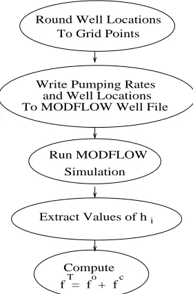
A MODFLOW simulation requires an input file containing the location and pumping rates of the wells in the model. If n > 5, each function evalu-ation requires a new set of pumping rates and thus the MODFLOW well file must be created each time the objective function is evaluated. Moreover, once the MODFLOW simulation is complete, the values of hi must be extracted
from the MODFLOW output file. A typical function evaluation is shown in Figure 2.
To generate the necessary data files to run MODFLOW we used the Groundwater
Modeling System (GMS), version 3.1. GMS is a modular interface to a
Write Pumping Rates and Well Locations
Run MODFLOW
Simulation Round Well Locations
To Grid Points
Compute f = f + fT o c Extract Values of hi
To MODFLOW Well File
Figure 2. Objective Function Evaluation
8. Numerical Results
We consider two formulations of the design space. For this work, the instal-lation cost of an extraction well, which is roughly $20,000, is high compared to the annual operating cost which is roughly $1,000. Since n = 5 wells extracting at Qemax = −0.0064(m3/s) satisfies the water supply demand (12) exactly, one obvious formulation is to fixn= 5and{Qi}5i=1 =−0.0064 and seek the optimal locations,{(xi, yi)}5i=1to minimize only the operational cost (foin (11)). We also include a formulation in which we start withN = 6
wells and seek the optimal locations and pumping rates to minimize (11), fT = fc+fo. Intuitively, since the installation cost is so high, we would
expect the five well configuration to have the lowest cost.
We examined the performance of one gradient-based code, the FDNIPS solver from the OPT++ v2.0 [33] framework. This code is a nonlinear interior point code based on the work in [17, 2, 3]. The code uses finite difference gradients, either trust region or line search globalization, and a choice of three merit functions. We tried several combinations of the options. In every case the optimization failed after 1000 calls to the function or failed because the line search had reduced the step length 40 times without a sufficient decrease in the merit function.
mu-tation operators, and the manner in which constraints are handled [36, 29]. Here, we consider a single-objective GA which incorporates both real- and binary-coded variables, and uses binary tournament selection [15]. For the real-coded variables, the simulated binary crossover (SBX) operator [15, 14] with polynomial mutation is used while single-point crossover with bitwise mutation are used for binary-coded variables.
An approach based on [12] is used to include constraints without the use of penalty parameters. Box constraints such as those in (13) are enforced automatically in the generation of candidate design variables, while a con-straint such as (12) is formulated as a non-negative functiong(Z) ≥0. The GA tournament selection process is then modified to account for the three scenarios: (1) when two feasible solutions are compared, the one with lower objective value is preferred; (2) when a feasible and infeasible solution are compared, the feasible one is taken; and (3) when two infeasible solutions are compared the one with lower overall constraint violation is preferred [12].
Parameters like the population size, number of generations, as well as the probabilities and distribution indexes chosen for the crossover and mutation operators effect the performance of a GA [36, 29]. For the purposes of our comparison, we wished to limit the number of simulations performed by the GA to a range of 2 to 3 times the number required by IFFCO. Since the total number of objective function evaluations is roughly the product of the population size and number of generations, this restricted our choices to fairly small populations and few generations. We also wished to use similar parameter values across the various problems. Although we did not perform a systematic study to find the best possible combinations, we experimented with a series of population sizes, numbers of generations, and crossover and mutation parameters to find a combination that gave representative perfor-mance for each of the problems we considered. Unless noted, the values used are listed Table III.
Table III. GA parameters
30 size of population 30 number of generations 0.9 crossover probability
0.1 real-coded mutation probability
20 distribution index for real-coded crossover 10 distribution index for real-coded mutation 0.5 binary-coded mutation probability 0.1 niching-parameter for constraints
8.1. SPATIALDISCRETIZATION
We use the same spatial discretization for both formulations. For the confined aquifer we discretize the domainΩ = [0,1000]×[0,1000]×[0,30](m) on an equally spaced50×50×10grid. For the unconfined aquifer, we used MOD-FLOW to determine the saturated domain Ωunc = [0,1000]×[0,1000]×
[0,27] ⊂ Ωand then discretized Ωunc on an equally spaced 50×50×10
grid.
8.2. FIVE WELL FORMULATION
8.2.1. Initial Iterate
0 100 200 300 400 500 600 700 800 900 1000 0
100 200 300 400 500 600 700 800 900 1000
x
y
52.5 52
51.5 51
50.5 50
49.5
Figure 3. Steady state head, confined aquifer
0 100 200 300 400 500 600 700 800 900 1000 0
100 200 300 400 500 600 700 800 900 1000
x
y
45
45
48
48 48
48.5 48.5
49 49
49.5
49.5
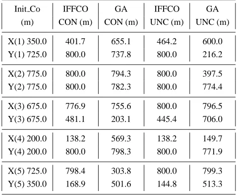
We refer to the confined aquifer as CON and unconfined aquifer as UNC. The function value at the initial iterate was $23,204 for CON and $26,958 for UNC. Table IV shows the minimum cost found and the number of calls to MODFLOW for both optimizers and aquifers. IFFCO reduced the cost by 6% for the confined aquifer and 11% for the unconfined aquifer. For both aquifers, the minimum cost found by the GA after 10 generations was 5% higher than the cost found by IFFCO–which is high considering the decrease from the initial iterate. Table V shows the initial x-y coordinates for the 5 wells and the optimal locations for each aquifer. The well locations at the optimal point lie on the boundary constraint, (15). This is physically rea-sonable, since the head values are higher in that region due to the Dirichlet boundary conditions. The GA’s cost was higher than IFFCO’s because well 5 in the confined case and well 1 in the unconfined case are not relocated close enough to the Dirichlet boundary conditions where the head values are higher.
In our evaluation of performance, we count only the expensive calls to the simulator as opposed to cumulative calls to the function. This is the approach taken in [6]. To see how this is a more realistic way to measure cost, consider the case where the linear constraint (12) is violated. One can detect this viola-tion, and return a failure forf, without calling the expensive flow simulator. IFFCO is being modified to make it easy for the user to evaluate cost at a finer granularity than this, to allow for the use of multiple simulators within the evaluation of the objective function and constraints. While this is a simple change in a serial code, correctly counting the calls to the various simulators in a parallel implementation requires considerable care.
Figure 5 is a plot of the value of the objective function against the cumu-lative number of calls to the simulator. IFFCO is currently being modified to allow the user to easily count calls to the objective function and calls to the individual simulators that are used to compute it. We set a function evaluation budget of 10,000 for this work and IFFCO converged to an optimal point within approximately 3% of the budget, terminating the optimization based on the sequence of finite difference scales. Figure 5 shows that after only roughly 100 function evaluations, the objective function does not decrease significantly.
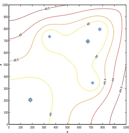
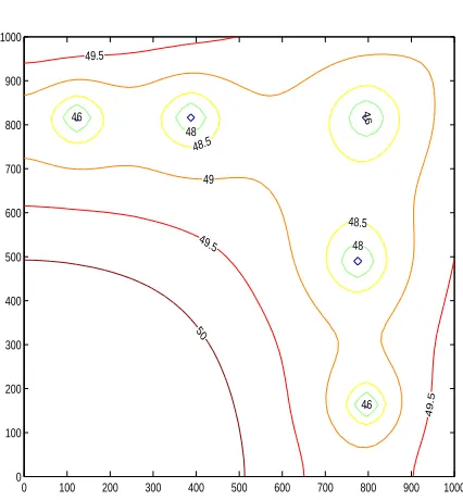
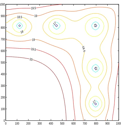
Figures 6 and 7 show the head contours in the layers containing the wells with the wells at the optimal locations.
8.3. SIX WELL FORMULATION
Table IV. Cost: 5 Wells
Optimizer Problem min f MODFLOW Calls
IFFCO CON $21,830 275
GA CON $22,822 330
IFFCO UNC $23,930 302
GA UNC $25,164 328
Table V. Optimal Locations
Init Co IFFCO GA IFFCO GA
(m) CON (m) CON (m) UNC (m) UNC (m)
X(1) 350.0 401.7 655.1 464.2 600.0 Y(1) 725.0 800.0 737.8 800.0 216.2
X(2) 775.0 800.0 794.3 800.0 397.5 Y(2) 775.0 800.0 782.3 800.0 774.4
X(3) 675.0 776.9 755.6 800.0 796.5 Y(3) 675.0 481.1 203.1 445.4 706.0
X(4) 200.0 138.2 569.3 138.2 149.7 Y(4) 200.0 800.0 798.3 800.0 771.9
X(5) 725.0 798.4 303.8 800.0 799.3 Y(5) 350.0 168.9 501.6 144.8 513.3
and pumping rates as decision variables. We included the installation cost (fc
in (11)) in the objective function for these runs. If the six well problem is initialized with all wells pumping at the maximum extraction rate, then one well is removed from the design in the course of the optimization and the minimum function value is within 0.2% of that found with the original five well configuration. If the six wells are initialized with
Qi=QminT /6, i= 1. . .6,
which is a feasible and sensible initial iterate, then a suboptimal point is found. All wells remain pumping close to the initial pumping rates, although the locations align with the specified head boundary conditions.
0 50 100 150 200 250 300 350 2.1
2.2 2.3 2.4 2.5 2.6 2.7x 10
4
Calls to MODFLOW
Function value
IFFCO CON GA CON IFFCO UNC GA UNC
Figure 5. Decrease in Function Values
0 100 200 300 400 500 600 700 800 900 1000 0
100 200 300 400 500 600 700 800 900 1000
46
48
48.5
49
49.5
50
46
49.5
49.5
46
48 48.5
Figure 6. Confined Aquifer
a mixed-integer formulation [37, 44, 30, 35]. Specifically, given the fact that fc was significantly larger than fo and that a minimum of five wells were
0 100 200 300 400 500 600 700 800 900 1000 0
100 200 300 400 500 600 700 800 900 1000
19.5 19 18.5
18
19
19.5
20
17
15
15
18.5
17
Figure 7. Unconfined Aquifer
s ranging from 1 to 8 in the GA’s formulation. A value of s in the range
1, . . . ,6resulted in shutting off the corresponding well, whiles = 7,8 led to six well designs. In addition, a well was removed from the design if its pumping rate fell below the installation threshold, regardless of the value of s. The unequal ranges associated with five and six well designs skewed the GA’s formulation to favor five-well designs. This reflected our heuristic that installing the minimum number of wells was likely to be cheaper than a six-well design.
Table VI shows the minimum cost and the number of calls to MODFLOW for both optimizers, aquifers for the better initial iterate. The cost at the initial iterate was $170,972 for the confined aquifer and $152,878 for the unconfined aquifer. Both the GA and IFFCO were able to remove one well from the design, resulting in a solution comparable to the five well configuration and reducing the cost by roughly 20%. For the suboptimal initial iterate, IFFCO was only able to decrease the cost 1%. The GA did not find anything bet-ter than the initial ibet-terate in 30 generations (over 100 function evaluations) for either aquifer with the suboptimal initial iterate included in the initial population.
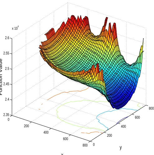
8.4. OPTIMIZATION LANDSCAPES
coordi-Table VI. Cost: 6 Wells
Optimizer Problem min f MODFLOW Calls
IFFCO CON $140,237 346
GA CON $140,628 464
IFFCO UNC $124,582 327
GA UNC $127,069 161
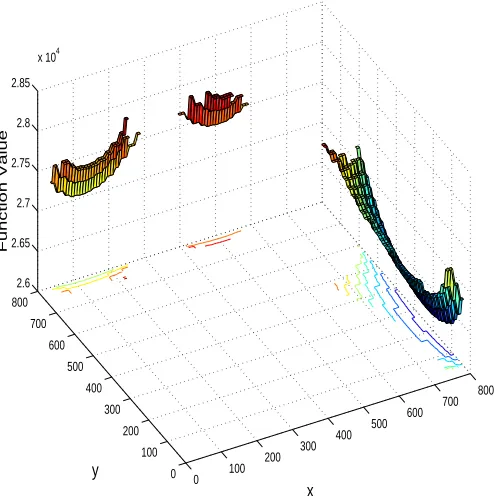
nates for well 1 vary between 20 and 800 meters. Figure 8 shows the cost landscape near the initial iterate for the confined aquifer and Figure 9 shows the landscape near the initial iterate for the unconfined aquifer. The peaks in the landscapes occur when two wells get close together, making the head values low and hence the operational cost higher. When two wells get too close they violate (14), leaving a small infeasible region inside each of the peaks. These peaks also make the landscapes nonconvex and introduce local minima. When we try to evaluate the function at an infeasible point, we do not plot an artificial value. Note that only a subset ofΩis feasible, especially for the unconfined aquifer near the initial iterate. The high infeasibility was due to repeated violation of the head constraint (14), which is why the unconfined case is more challenging. There are also small discontinuities apparent in the landscapes since we round real numbers to grid locations to run the flow simulator.
0
200
400
600
800 0
200 400
600 800 2.25
2.3 2.35 2.4 2.45 2.5 2.55 2.6
x 104
y x
Function Value
Figure 8. Landscape near initial iterate: confined aquifer
0 100
200 300
400 500
600 700
800
0 100 200 300 400 500 600 700 800
2.6 2.65 2.7 2.75 2.8 2.85
x 104
x y
Function Value
0
200
400
600
800 0
200 400
600 800 2.26
2.28 2.3 2.32 2.34 2.36
x 105
Figure 10. Landscape near solution: confined aquifer
0
200 400
600
800 0
200 400
600 800
2.35 2.4 2.45 2.5 2.55 2.6
x 104
y x
Function Value
8.5. DISCUSSION
•The numerical results indicate that the six well formulation is much more difficult than the five well formulation since one well must be removed from the design while the remaining wells extract at the maximum extraction rate. IFFCO did well on the the six well formulation with an initial iterate with all wells extracting at the maximum rate. In the other case a local minimum is found. With or without the mixed-integer formulation, the six well problem proved difficult for the GA, since removing a well only led to a feasible iterate if the other five were pumping at the maximum rate. The GA was able to find a feasible five well solution when the better initial iterate was included as a member of the initial population. With a completely random initial population or with the sub-optimal initial iterate included, the GA solution for the con-fined aquifer problem was a sub-optimal six well design. The same was true for the unconfined case. However, the GA with a completely random popu-lation was unable to find a feasible iterate for the unconfined problem even when using a population size of two hundred and running for two hundred generations.
• We also considered the possibility that, over a longer time period, the six well model with the suboptimal initial iterate may be superior to the five well model. We ran both the confined and unconfined problems for one year to determine the annual operational cost. One can see that a time of roughly 130 years for the confined aquifer and 90 years for the unconfined aquifer is needed to obtain a lower using the six well model. Hence the five well results are the most realistic. We ran both problems again with the longer time horizons to confirm that the six well model would outperform the five well model.
for the confined aquifer design wasfT =$161,588 after 510 function
eval-uations, while the unconfined aquifer solution had a cost of fT =$142,755 after 359 function evaluations.
• This application is challenging for formulations withN > 5 wells since wells must be removed from the design space to decrease the installation cost. Removing wells from the design is an active area of research and numerous approaches exist for approximating fixed costs with continuous functions (see [32] and the references therein). Our approach for removing a well if |Qi| <10−4results in a discontinuous fixed cost. This approach was
9. Conclusions
This work was an initial analysis of a subset of the community problems pro-posed in [30]. The formulation of the objective function and constraints are discontinuous and have local minima as the optimization landscapes verify. These features are the reason for the failure of the gradient-based method (see § 8). As pointed out in [30], deterministic sampling methods have not been used to their full potential in the subsurface optimization community. In this work we found a solution to the well-field design application with the implicit filtering algorithm and we compared our results to those obtained with a simple genetic algorithm.
We found these problems to be challenging for several reasons. A minimal cost is obtained with few wells pumping at large rates. For these problems, local minima exist when more wells are extracting at low costs. A large decrease in the objective function occurs when a well is removed from the design space. The installation cost for this work is discontinuous, yet we found that with good initial data, that the implicit filtering algorithm could perform well despite the discontinuous formulation for N < 9. Another challenge is that the feasible region, especially for the unconfined aquifer, is small. Although implicit filtering started with a feasible initial iterate, much experimental work was done to find one. The genetic algorithm was unable to find a feasible point for the six well formulation and required a feasible point in the initial population in order for the optimization to progress for the unconfined aquifer.
We can extend this study to improve the solution for this type of problem. •IFFCO requires a feasible initial iterate, and the numerical results show that a good initial iterate is needed for the optimization. Surrogate models based on statistical sampling [5, 6] may be a good way to explore design space for good initial iterates.
• As pointed out in [30], a more accurate realization of the subsurface is needed for solutions of this class of problems to be used in decision making. Adding heterogeneities to the domain would create a more realistic snap-shot of the subsurface yet would make the optimization landscapes much more challenging. More robust optimization techniques may be needed as the conceptual domain becomes more realistic.
•We used MODFLOW to simulate flow for a well-field design application, despite the simulator’s simple well model. The real-valued well location that is output from the optimizer is rounded to a grid location. For a more accurate solution, a simulator that is able to more accurately resolve flow around the well is essential. A well model that need not place wells at the center of a cell would be ideal.
that use a surrogate response surface, is currently being done and is necessary before any solid conclusions can be made on which method performs best for this class of problems.
10. Downloading and Running the Test Problems
The problems can be obtained from
http://www4.ncsu.edu/˜ctk/community.html
The test problems are packaged as compressed UNIX tar files. The serial codes are for the g77 compiler and have been tested on SUN SparcStations running Solaris, various Intel platforms running Red Hat Linux 7.3 and 8.0, and an Apple Macintosh G4 running OSX 10.2. The MPI version of the codes has been tested on an IBM-SP3 and a DELL Linux server. IFFCO is included in the packages. The README files in the main directory explain how to assemble the files and interpret the results.
MODFLOW can be obtained directly from the USGS at the URL
http://water.usgs.gov/software/modflow-96.html
The USGS provides compiled executables for SUN, SGI, and DOS sys-tems, as well as UNIX source. Our packages provide makefiles for some other UNIX environments.
Acknowledgments
The research of KRK, CEK, CTK, RWD, and JPR was supported in part by National Science Foundation grants DMS-0070641, DMS-0112542, Army Research Office grants DAAD19-02-1-0391 and DAAD19-02-1-0111, and a Department of Education GAANN fellowship. The research of CTM and MWF was partially supported by National Institute of Environmental Health Sciences grant P42 ES05948-02 and National Science Foundation grant DMS-0112653. Partial support of this work was also provided by the National Science Foundation through DMS-0112069 to the Statistical and Applied Mathematical Sciences Institute in Research Triangle Park, where a portion of this work was done. Some of the computational support was provided by the North Carolina Supercomputing Center.
References
1. Aly, A. H. and R. C. Peralta: 1999, ‘Comparison of a genetic algorithm and mathematical programming to the design of groundwater cleanup systems’. Water Resources Research
35(8), 2415–2425.
2. Argaez, M. and R. A. Tapia: 2001, ‘On the Global Convergence of a Modified Augmented Lagrangian Linesearch Interior-Point Newton Method for Nonlinear Pro-gramming’. J. Optim. Theory Appl. 114, 1–25.
3. Argaez, M., R. A. Tapia, and L. Velazquez: 2002, ‘Numerical Comparisons of Path-Following Strategies for a Primal-Dual Interior-Point Method for Nonlinear Program-ming’. J. Optim. Theory Appl. 114, 255–272.
4. Battermann, A., J. M. Gablonsky, A. Patrick, C. T. Kelley, T. Coffey, K. Kavanagh, and C. T. Miller: 2002, ‘Solution of A Groundwater Control Problem with Implicit Filtering’.
Optimization and Engineering 3, 189–199.
5. Booker, A. J.: 1994, ‘DOE for computer output’. Technical Report BCSTECH-94-052, Boeing Computer Services, Seattle, WA.
6. Booker, A. J., J. E. Dennis, P. D. Frank, D. B. Serafini, V. Torczon, and M. W. Trosset: 1999, ‘A rigorous framework for optimization of expensive functions by surrogates’.
Structural Optimization 17, 1–13.
7. Broyden, C. G.: 1967, ‘Quasi-Newton methods and their application to function minimization’. Math. Comp. 21, 368–381.
8. Broyden, C. G.: 1969, ‘A new double-rank minimization algorithm’. AMS Notices 16, 670.
9. Carter, R., J. M. Gablonsky, A. Patrick, C. T. Kelley, and O. J. Eslinger: 2001, ‘Algo-rithms for Noisy Problems in Gas Transmission Pipeline Optimization’. Optimization
and Engineering 2, 139–157.
10. Choi, T., O. Eslinger, P. Gilmore, C. Kelley, and H. Patrick: 2001, ‘User’s guide to IFFCO’.
11. Choi, T. D. and C. T. Kelley: 2000, ‘Superlinear Convergence and Implicit Filtering’.
SIAM J. Optim. 10, 1149–1162.
12. Deb, K.: 2000, ‘An efficient constraint handling method for genetic algorithms’.
Computer Methods in Applied Mechanics and Engineering 186(2–4), 311–338.
13. Deb, K.: 2003, ‘KanGal Homepage’. Indian Institute of Technology Kanpur http://www.iitk.ac.in/kangal.
14. Deb, K. and H. Beyer: 2001, ‘Self-Adaptive Genetic Algorithms with Simulated Binary Crossover’. Evolutionary Computation Journal 9(2), 197–221.
15. Deb, K. and A. R.B.: 1995, ‘Simulated binary crossover for continuous search space’.
Complex Systems 9, 115–148.
16. Dennis, J. E. and V. Torczon: 1991, ‘Direct Search Methods on Parallel Machines’. SIAM
J. Optim. 1, 448 – 474.
17. El-Bakry, A. S., R. A. Tapia, T. Tsuchiya, and Y. Zhang: 1996, ‘On the formulation and theory of the Newton interior-point method for nonlinear programming’. J. Optim.
Theory Appl. 89, 507–541.
18. Fiacco, A. V. and G. P. McCormick: 1990, Nonlinear Programming, No. 4 in Classics in Applied Mathematics. Philadelphia: SIAM.
19. Fletcher, R.: 1970, ‘A new approach to variable metric methods’. Comput. J. 13, 317– 322.
20. Gilmore, P.: 1993, ‘An Algorithm for Optimizing Functions with Multiple Minima’. Ph.D. thesis, North Carolina State University, Raleigh, North Carolina.
22. Goldfarb, D.: 1970, ‘A family of variable metric methods derived by variational means’.
Math. Comp. 24, 23–26.
23. Hooke, R. and T. A. Jeeves: 1961, ‘Direct search solution of numerical and statistical problems’. Journal of the Association for Computing Machinery 8, 212–229.
24. Huang, C. and A. S. Mayer: 1997, ‘Pump-and-treat optimization using well locations and pumping rates as decision variables’. Water Resources Research 33(5), 1001–1012. 25. Jones, D. R., C. C. Perttunen, and B. E. Stuckman: 1993, ‘Lipschitzian Optimization
Without the Lipschitz Constant’. J. Optim. Theory Appl. 79, 157–181.
26. Kelley, C. T.: 1999, Iterative Methods for Optimization, Vol. 16 of Frontiers in Applied
Mathematics. Philadelphia, PA: SIAM, first edition.
27. Lewis, R. M. and V. Torczon: 2000, ‘Pattern Search Algorithms for Linearly Constrained Minimization’. SIAM J. Optim. 10, 917–941.
28. Marryott, R. A., D. E. Dougherty, and R. L. Stollar: 1993, ‘Optimal Groundwater Man-agement .2. Application of Simulated Annealing to a Field-Scale Contamination Site’.
Water Resources Research 29(4), 847–860.
29. Mayer, A., C. Kelley, and C. Miller: 2002a, ‘Optimal design for problems involving flow and transport phenonmena in saturated subsurface systems’. Advances in Water
Resources 12, 1233–1256.
30. Mayer, A. S., C. T. Kelley, and C. T. Miller: 2002b, ‘Optimal Design for Problems Involving Flow and Transport Phenomena in Saturated Subsurface Systems’. Advances
in Water Resources 12, 1233–1256.
31. McDonald, M. and A. Harbaugh: 1988, ‘A Modular Three Dimensional Finite Differ-ence Groundwater Flow Model’. U.S. Geological Survey Techniques of Water Resources
Investigations.
32. McKinney, D. C. and M.-D. Lin: 1995, ‘Approximate Mixed-Integer Nonlinear Pro-gramming Methods for optimal Aquifer Remediation Design’. Water Resources Research 31, 731–740.
33. Meza, J. C.: 1994, ‘OPT++: An Object-Oriented Class Library for Nonlinear Optimiza-tion’. Technical Report SAND94-8225, Sandia National Laboratory.
34. Nelder, J. A. and R. Mead: 1965, ‘A simplex method for function minimization’.
Comput. J. 7, 308–313.
35. Reed, P.: 2003. private communication.
36. Reed, P., B. Minsker, and D. Goldberg: 2000, ‘Designing a competent simple genetic algorithm for search and optimization’. Water Resources Research 36(12), 3757–3761. 37. Ritzel, B., J. Eheart, and S. Ranjithan: 1994a, ‘Using genetic algorithms to solve a
mul-tiple objective groundwater pollution containment problem’. Water Resources Research
30(5), 1589–1604.
38. Ritzel, B. J., J. W. Eheart, and S. Ranjithan: 1994b, ‘Using Genetic Algorithms to Solve a Multiple Objective Groundwater Pollution Containment Problem’. Water Resources
Research 30(5), 1589–1603.
39. Rizzo, D. M. and D. E. Dougherty: 1996, ‘Design optimization for multiple management period groundwater remediation’. Water Resources Research 32(8), 2549–2561. 40. Rogers, L. L. and F. U. Dowla: 1994, ‘Optimization of Groundwater Remediation Using
Artificial Neural Networks with Parallel Solute Transport Modeling’. Water Resources
Research 30(2), 457–481.
41. Shanno, D. F.: 1970, ‘Conditioning of quasi-Newton methods for function minimiza-tion’. Math. Comp. 24, 647–657.
42. Stoneking, D., G. Bilbro, R. Trew, P. Gilmore, and C. T. Kelley: 1992, ‘Yield Opti-mization Using a GaAs Process Simulator Coupled to a Physical Device Model’. IEEE
43. Torczon, V.: 1989, ‘Multidirectional Search’. Ph.D. thesis, Rice University, Houston, Texas.
44. Watkins Jr, D. and D. McKinney: 1998, ‘Decomposition methods for water resources optimization models with fixed costs’. Advances in Water Resources 21(4), 261–324. 45. Zheng, C. and P. P. Wang: 1999, ‘An integrated global and local optimization approach