Short Term Electric Load Forecasting.

(1)

ABSTRACT

HONG, TAO. Short Term Electric Load Forecasting. (Under the direction of Simon Hsiang and Mesut Baran).

Load forecasting has been a conventional and important process in electric utilities since the early 20th century. Due to the deregulation of the electric utility industry, the utilities tend to be conservative about infrastructure upgrade, which leads to stressed utilization of the equipment. Consequently, the traditional business needs of load forecasting, such as planning, operations and maintenance, become more crucial than before. In addition, participation in the electricity market requires the utilities to forecast their loads accurately. Nowadays, with the promotion of smart grid technologies, load forecasting is of even greater importance due to its applications in the planning of demand side management, electric vehicles, distributed energy resources, etc.

(2)

(3)

Short Term Electric Load Forecasting

by Tao Hong

A dissertation submitted to the Graduate Faculty of North Carolina State University

in partial fulfillment of the requirements for the degree of

Doctor of Philosophy

Operations Research and Electrical Engineering

Raleigh, North Carolina 9/10/2010

APPROVED BY:

_______________________________ ______________________________

Simon M Hsiang Mesut E Baran

(4)

Dedication

(5)

Biography

(6)

Acknowledgements

As a graduate student who has gone through 5 years of graduate school with nearly 40 courses across 7 programs, I’ve seen too many peers suffering with the following Q&A’s:

Q: Why PhD?

A: I have no choice. I can’t find a job. Q: Why this research topic?

A: I have no choice. My advisor asked me to work on it.

(7)

Dr. Simon Hsiang, who was master thesis advisor and now my PhD advisor, is the first one to educate me what the meaning of Ph.D. is. Although the research direction I finally decided to go to is not what he is interested in, he still offered me tremendous constructive comments and insights, of which “As long as it’s good science” has always been his justification. Thank Dr. Hsiang for granting me total freedom all the way. It’s also my fortune that Dr. Hsiang trusts my capability, which cannot be more encouraging to me during my research.

Dr. Mesut Baran is the first one to lead me to the field of power systems. I highly appreciate his course ECE550, the first power systems course I took, which helped build my fundamental background of power system analysis. Also many thanks to Dr. Baran for the suggestion of putting ANN into the comparative assessment, which made the dissertation as well rounded as it is now.

(8)

papers were produced by irresponsible researchers, and keeping me from being one of them.

Dr. Dickey is the first one to introduce me to time series analysis. The first time I took his lecture, I said to myself: “This subject has to be appreciated by the load forecasting guys in the way he presented.” It’s my honor to have Dr. Dickey on my committee. I will always be grateful that there has been a Nobel citation professor who read my dissertation draft word-by-word and offered the revision comments in great detail.

Dr. Richard Brown, the greatest boss I’ve ever experienced, is the first one to bring me to the utility industry, and also the first person that encouraged me to pursue a degree in OR. It’s so unfortunate that he was not able to attend my final oral exam. However, my research wouldn’t be as valuable as it is to the industry without Dr. Brown’s advice since day one. I also greatly appreciate the career guidance and flexible working environment he offered me.

(9)

portion of this priceless project, of which most materials became part of the contents in this dissertation.

(10)

List of Tables

Table 1.1 Needs of forecasts in utilities. ... 5

Table 1.2 Availability of temperature, economics, and land use information. ... 9

Table 1.3 Classification of load forecasts. ... 9

Table 1.4 Applications of the forecasts. ... 9

Table 2.1 Day type codes appeared in the literature. ... 47

Table 3.1 Conceptual differences between MLR and PLR ... 64

Table 4.1 Benchmark candidates ... 89

Table 4.2 MAPEs of the seven benchmarking model candidates. ... 90

Table 4.3 MAPEs of the Recency Effect Candidates ... 96

Table 4.4 MAPEs of the Weekend Effect Candidates ... 100

Table 4.5 US Public Holidays Established by Federal Law (5 U.S.C. 603) ... 102

Table 4.6 MAPEs of the Alternatives for the Six Fix-Weekday Holidays ... 107

Table 4.7 MAPEs of the Alternatives for the Surrounding Days of Memorial Day and Labor Day ... 107

Table 4.8 MAPEs of the Alternatives for the Four Fix-Date Holidays ... 108

Table 4.9 MAPEs of the Days After the Three Significant Fix-Date Holidays ... 108

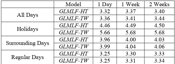
Table 4.10 GLMLF-HT vs. GLMLF-TW ... 109

(15)

Table 4.12 MAPEs of the five milestone models ... 111

Table 4.13 One Week Ahead Forecasting Performance for All Milestones ... 112

Table 4.14 Effectiveness of Holiday Effect Modeling of GLMSTLF-HT ... 113

Table 4.15 MAPEs of GLMSTLF-HT in Special Hours ... 115

Table 4.16 DSM activities (2001 – 2008) ... 116

Table 4.17 MAPEs of the Five Milestone Models (Preprocessed Data). ... 117

Table 4.18 One Week Ahead Forecasting Performance Comparison (GLMSTLF-HT) ... 118

Table 5.1 MAPEs of the seven PLM based benchmarking model candidates. ... 120

Table 5.2 MAPEs of the seven PLM based benchmarking model candidates (preprocessed data). ... 123

Table 5.3 Data for numerical examples. ... 124

Table 5.4 Seven numerical examples. ... 133

Table 6.1 MAPEs of ANNLF-S. ... 138

Table 6.2 MAPEs of ANNLF-BS. ... 139

Table 6.3 MAPEs of ANNLF-HTS... 140

Table 6.4 MAPEs of ANNLF-BM. ... 141

Table 6.5 MAPEs of ANNLF-HTM. ... 142

(16)

(17)

List of Figures

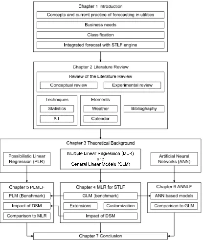
Figure 1.1 Organization of the dissertation... 13

Figure 2.1 A typical STLF process. ... 15

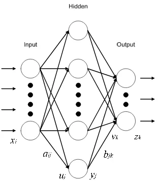
Figure 3.1 A three-layer feed-forward artificial neural network. ... 71

Figure 4.1 Load series (2005-2008). ... 83

Figure 4.2 Temperature series (2005-2008). ... 83

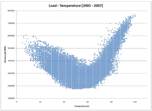
Figure 4.3 Load-temperature scatter plot (2005-2008). ... 84

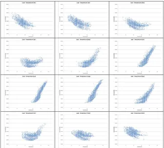
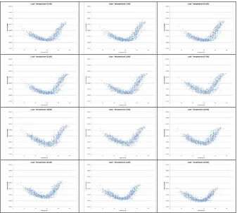
Figure 4.4 Load-temperature scatter plots for 12 months. ... 86

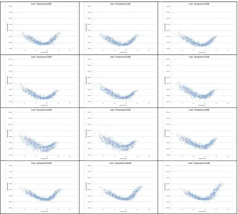
Figure 4.5 Load-temperature scatter plots (Hours 1 to 12). ... 87

Figure 4.6 Load-temperature scatter plots (Hours 13 to 24). ... 88

Figure 4.7 Normalized hourly load profile of a week. ... 100

Figure 4.8 The annual peak day of 2009. ... 115

Figure 5.1 Data for the numerical examples. ... 125

Figure 5.2 Example 1: PLM underperforms GLM. ... 127

Figure 5.3 Example 2: PLM underperforms GLM. ... 128

Figure 5.4 Example 3: PLM outperforms GLM. ... 129

Figure 5.5 Example 4: PLM outperforms GLM. ... 130

Figure 5.6 Example 5: PLM ties with GLM. ... 131

(18)

(19)

1 Introduction

(20)

1.1 Forecasting in Electric Utilities

In many organizations, planning and forecasting are seamlessly integrated together. Therefore, the forecasting function of a utility is normally assigned to the planning department. Nevertheless, the distinction between the two should not be omitted. Planning provides the strategies, given certain forecasts, whereas forecasting estimates the results, given the plan. Planning relates to what the utility should do. Forecasting relates to what will happen if the utility tries to implement a given strategy in a possible environment. Forecasting also helps to determine the likelihood of the possible environments.

(21)

1.2 Business Needs of Load Forecasts

In today’s world, load forecasting is an important process in most utilities with the applications spread across several departments, such as planning department, operations department, trading department, etc. The business needs of the utilities can be summarized, but not limited to, the following:

1) Energy purchasing. Whether a utility purchases its own energy supplies from the market place, or outsources this function to other parties, load forecasts are essential for purchasing energy. The utilities can perform bi-lateral purchases and asset commitment in the long term, e.g., 10 years ahead. They can also do hedging and block purchases one month to 3 years ahead, and adjust (buy or sell) the energy purchase in the day-ahead market.

(22)

3) Operations and maintenance. In daily operations, load patterns obtained during the load forecasting process guide the system operators to make switching and loading decisions, and schedule maintenance outages.

4) Demand side management (DSM). Although lots of DSM activities are belong to daily operations, it is worthwhile to separate DSM from the operations category due to its importance in this smart-grid world. A load forecast can support the decisions in load control and voltage reduction. On the other hand, through the studies performed during load forecasting, utilities can perform long term planning according to the characteristics of the end-use behavior of certain customers.

5) Financial planning. The load forecasts can also help the executives of the utilities project medium and long term revenues, make decisions during acquisitions, approve or disapprove project budgets, plan human resources and technologies, etc.

(23)

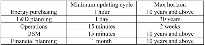
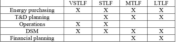
Table 1.1 Needs of forecasts in utilities.

Minimum updating cycle Max horizon

Energy purchasing 1 hour 10 years and above

T&D planning 1 day 30 years

Operations 15 minutes 2 weeks

DSM 15 minutes 10 years and above

(24)

1.3 Classification of Load Forecasts

There is no single forecast that can satisfy all of the needs of utilities. A common practice is to use different forecasts for different purposes. The classification of various forecasts is not only depending upon the business needs of utilities, but also the availability of the crucial elements that affect the energy consumption: weather (or climate in the long periods) and human activities.

Weather refers to the present condition of the meteorological elements, such as temperature, humidity, wind, rainfall, etc., and their variations in a given region over periods up to two weeks. Climate encompasses these same elements in a given region and their variations over long periods of time. The uses of various weather variables will be discussed in the next chapter. Since temperature has the most impact to energy consumption among all the meteorological elements, all the models developed in this report use temperature information only. Nevertheless, the methodology can be applied to other meteorological elements. Nowadays, for load forecasting purpose, temperature forecast can be relatively accurate up to one day ahead, and be inaccurate but reliable up to two weeks ahead.

(25)

impact varies on different economical conditions. For instance, during the year of 2009, which is the early part of a recession in US, the energy consumption of US is lower than that of 2008, because people were using power more conservatively, and lots of businesses were closed. With the advancement of econometric techniques, the economics information can be relatively accurate up to one year ahead, and be inaccurate but reliable up to 3 years ahead for load forecasting purpose. In the annual resolution, both climate and economics can affect the energy consumption. However, due to the unavailability of both inputs, the system level load forecast can be only obtained by simulating various scenarios. On the other hand, the long term energy consumption on the circuit level is affected by urban development, which can be realized by land use changes. The land use information is normally accurate within one year, inaccurate but reliable up to 5 years. Although some counties can provide a 30 years ahead urban development plan, it is still not clear what exactly would happen year by year during the next 30 years. Forecasting the load on the circuit level with land use simulation is called spatial electric load forecasting [89].

(26)

load forecasting (STLF), medium term load forecasting (MTLF), and long term load forecasting (LTLF).

(27)

Table 1.2 Availability of temperature, economics, and land use information.

Accurate Inaccurate Unreliable

Temperature 1 day 2 weeks > 2 week

Economics 1 month 3 years > 3 years

Land use 1 year 5 years > 5 years

Table 1.3 Classification of load forecasts.

Temperature Economics Land Use Updating Cycle Horizon

VSTLF Optional Optional Optional <= 1 Hour 1 day

STLF Required Optional Optional 1 Day 2 weeks

MTLF Simulated Required Optional 1 month 3 years

LTLF Simulated Simulated Required 1 year 30 years

With the classification of load forecasts shown in Table 1.3, we can associate each forecast to the business needs of the utilities and the corresponding lead time, which are shown in Table 1.4. Due to the wide span of updating cycle and horizon, one business need may be tied to several forecasts. For instance, an energy purchasing contract may be one day ahead, one year ahead, or 10 years ahead, where load forecasts from very short term to long term can be applied.

Table 1.4 Applications of the forecasts.

VSTLF STLF MTLF LTLF

Energy purchasing X X X X

T&D planning X X X

Operations X X

(28)

1.4 Integrated Forecasting with a STLF Engine

Although several departments in a utility may share the same type of forecasts, usually there is not much communication among them in the current practice, which results in inefficient utilization of resources. Not only are human resources used redundantly, producing the same forecast in various departments, but also the quality of these forecasts may vary due to the lack of communication and information sharing. For instance, on STLF, operations department may use SCADA data, which may not be as accurate as the billing data used by the trading department. On the other hand, the trading department may not know about an ongoing outage, which would result in a less accurate forecast for the next few hours.

This dissertation develops a novel regression-based STLF engine for an integrated load forecasting process. The term “integrated” here refers to initiating all the forecasts from the same department with the same methodology and engine. STLF is selected as the engine and base of the integrated forecasting process due to its inherent connectivity to other types of forecasts:

(29)

future residuals and adding them back to the short term forecast, a very short term forecast can be obtained.

2) STLF to MTLF & LTLF: by adding econometrics variables to the STLF model and extrapolating the model to the longer horizon, the system level MTLF and LTLF can be obtained. Consequently, this long term system level load forecast can be used as an input for long term spatial load forecasting. The rest of this dissertation is mainly devoted to the STLF model development. The organization of this dissertation is shown in Figure 1.1. Chapter 2 presents a comprehensive literature review of STLF. Chapter 3 introduces the theoretical background of three techniques, multiple linear regression (MLR) – one of the earliest and most widely applied techniques in STLF, possibilistic linear regression (PLR) – one of the most recently applied techniques in STLF, and artificial neural networks (ANN) – one of the most popular techniques in STLF. Chapter 4 develops several general linear model (GLM) based load forecasters1 starting from a base model (GLMLF-B) for benchmarking purposes. The extensions of this base model are demonstrated. Then it is customized by modeling several special effects. Chapters 5 and 6 develop the possibilistic linear models (PLMs) and ANNs for load forecasting respectively. The focus is on the comparisons to the GLMs. Through the comparative assessment, ways to utilize and improve PLR and ANN for STLF are discussed. The

(30)

(31)

(32)

2 Literature Review

(33)

2.1 Overview

Figure 2.1 shows a typical STLF process conducted in the utilities that rely on the weather information. Weather and load history are taken as the inputs to the modeling process. After the parameters are estimated, the model and weather forecast are extrapolated to generate the final forecast. A time series, including the load series, can be decomposed to systematic variation and noise. The modeling process in Figure 2.1 tends to capture the systematic variation, which, as an input to the extrapolating process, is crucial to the forecast accuracy. As a consequence, a large variety of pioneer research and practices in the field of STLF has been devoted to the modeling process. Most of the model development work can be summarized from two aspects: techniques and variables.

Figure 2.1 A typical STLF process.

(34)

analysis [66] and time series analysis [28], and artificial intelligence (AI) based approaches, such as ANN [31], fuzzy logic (FL) [74], and support vector machine (SVM) [10]. Various combinations of these techniques have also been studied and applied to STLF problems.

On the other hand, people have been seeking the most suitable variables for each particular problem and trying to generalize the conclusions to interpret the causality of the electric load consumption. Most of these efforts were embedded coherently into the development of the techniques. For instance, temperature and relative humidity were considered in [48], while The effect of humidity and wind speed were considered through a linear transformation of temperature in the improved version [49]. In general, the electric load is mainly driven by nature and human activities. The effects of nature are normally reflected by weather variables, e.g., temperature, while the effects of human activities are normally reflected by the calendar variables, e.g., business hours. The combined effects of both elements exist as well but are nontrivial.

(35)

proposed, of which the results are reported to be superior to an existing STLF program [50]. Since the price-sensitive environment is not generic in the current US utility industry, price information was not included in Figure 2.1 or the scope of this report.

Although the majority of the literature in STLF is on the modeling process, there is some research concerning other aspects to improve the forecast. Weather forecast, as an input to the extrapolating process, is also very important to the accuracy of STLF. Consequently, another branch of research work is focusing on developing, improving or incorporating the weather forecast [32]. A temperature forecaster is proposed for STLF [47]. Front-end weather forecast is incorporated in the STLF system to improve the forecasting performance [61].

(36)

2.2 Review of the Literature Reviews

2.2.1 Conceptual Reviews

The literature of load forecasting can be traced back to at least 1918 [44, 76]. In the early 1980s, the Load Forecasting Working Group of IEEE published two papers to compile the load forecasting bibliography [44, 58]. To emphasize the modern developments in STLF, most of the papers reviewed in this chapter are published after 1980. In the past 40 years, the developments in STLF have been reviewed by many researchers from various perspectives. These literature reviews can be roughly categorized into two groups by whether there are experiments conducted during the review or not. The ones without experiments, or conceptual reviews, tend to review the literature on the conceptual level based on the developments, results, and conclusions from the original papers [1, 27, 31, 60]. The ones with experiments, or experimental reviews, tend to implement, analyze, evaluate, and compare the different techniques reported in the literature using one or several new sets of data [32, 57, 62, 88].

(37)

identification part of STLF. The merits and drawbacks of each approach are discussed in the review. Among the techniques being reviewed, the authors claimed that time series and state-space approaches were extensively used for STLF at that time. Both techniques had strong theoretical foundations. The time series models were easy to understand and apply, were good at accommodating the cyclic behavior of the load, but were difficult to update online at the time the paper was written. The state-space technique was well-suited for online application, but could not easily include the weather variables. The multivariable load modeling was the most favorable technique by the authors but did not receive much attention from the field at that time due to the difficulty level of understanding and applying them.

A major concern of some techniques reviewed by Abu-El-Magd and Sinha was the suitability for online application. Three decades ago, as what they pointed out, it required a long time to do offline analysis using the multiple regression approach, and it took a long time to update the parameters for the time series models. However, with the modern computing environment, these methods can be easily deployed for online STLF with no timing issue.

(38)

functions of an energy management system (EMS) was emphasized. The paper very well summarized the factors that affected the electricity consumption, and classified some popular load modeling and forecasting techniques. The authors also provided a detailed discussion regarding the practical aspects of the development and usage of STLF models and packages.

In Gross and Galiana’s review, it was reported that the pure time-of-day models, or similar day method (use the load of a past similar day as the forecasted load), were being replaced by the dynamic models, such as time series models and state-space models. The computational time for the dynamic models was not a major consideration in the review. Two missing components in the STLF literature were mentioned in this review: experience of actual data, particularly in an online environment, and the comparative study of various STLF approaches on a set of standard benchmark systems.

(39)

real data, most of the tests reported by the papers within the review were not systematically carried out. Some of them did not provide comparison to standard benchmarks, and some did not follow standard statistical procedures in reporting the analysis of errors.

Another contribution of Hippert’s review is to summarize the issues in designing a STLF system using the ANN based approaches. The design tasks are divided into four stages: data pre-processing, ANN design, implementation, and validation. In the ANN design stage for forecasting load profiles, the authors summarize three ways most people do: iterative forecasting, multi-model forecasting, and single-model multivariate forecasting. In the iterative forecasting, the forecasts for the later hours will be based on those of the earlier ones. The concept is similar to Box-Jenkins time series models, but it is not clear whether the forecast series will converge to the series average. In the multi-model forecasting, several ANN models are used in parallel to forecast the load series, e.g., 24 ANNs can be used to forecast the loads of the next 24 hours. This method is common for load forecasting with regression models as pointed out by the authors. In the single-model multivariate forecasting, all the loads are forecasted at once through a multivariate method. The author pointed out two drawbacks of implementing this idea in ANN.

(40)

as expert systems (ES), ANN, and the genetic algorithm (GA) in STLF [60]. The survey summarized the development of each technique chronically. Advantages of AI techniques in STLF were summarized conceptually and qualitatively. No detailed disadvantages were discussed in the content. Without any solid support, the paper claimed that the AI techniques to “have matured to the point of offering real practical

benefits in many of their applications”, which is beyond the scope of this paper

defined by the authors. On the other hand, the authors include “sharing thoughts and

estimations on AI future prospects” in STLF as a scope. However, few tangible or

(41)

2.2.2 Experimental Reviews

Five techniques were evaluated in [62]: multiple linear regression, stochastic time series, general exponential smoothing, state space method, and knowledge-based approach. The significance of the paper was in the comparative analysis of the five techniques, which would help the new researchers and practitioners in the field of STLF “get an understanding of their inherent level of difficulty and the expected

results”. The authors implemented the five techniques to generate an hourly,

24-hour-ahead load forecast using the data from a southeastern utility in US. The implementation of each technique is briefly described and the results are compared and analyzed with recommendations from the authors. The paper very well served the scope defined by the author. Since the authors did not pursue the best model for each technique, no conclusion can be drawn regarding the comparison of the ultimate performance of each one.

(42)

work. On the other hand, the design and implementation of FL-based and NN-based forecasters were not explained clearly, which further devalued the contribution and significance of this paper.

(43)

2.3 Statistical Approaches

2.3.1 Regression Analysis

A regression-based approach to STLF is proposed by Papalexopoulos and Hesterberg [66]. The proposed approach was reported to be tested using Pacific Gas and Electric Company’s (PG&E) data for the peak and hourly load forecasts of the next 24 hours. This is one of the few papers fully focused on regression analysis for STLF in the past 20 years [29, 45, 75]. Some modeling concepts of using multiple linear regression for STLF were applied: weighted least square technique, temperature modeling by using heating and cooling degree functions, holiday modeling by using binary variables, and a robust parameter estimation method etc. Through a thorough test, the new model was concluded to be superior to the existing one used in PG&E.

(44)

obtain a more robust forecast was not quite justifiable. This very issue was also pointed out by Larson in the appended discussion of this paper, and the authors’ response did not show much strong evidence to support their statement.

(45)

Electric Power Utility of Serbia, was deployed in the dispatching center of the same utility for one to seven days ahead load forecast.

(46)

2.3.2 Time Series Analysis

Regression techniques were combined with ARIMA models for STLF in [54]. Regression techniques were used to model and forecast the peak and trough load, as well as weather normalize the load history, or “remove the weather-sensitive trend” from the load series. Then ARIMA was applied to a weather normalized load to produce the forecast. Finally the forecasted normalized load was adjusted based on the forecasted peak and trough load.

ARIMA models, together with other Box and Jenkins time series models were applied to STLF shown to be ”well suited to this application” in Hagan and Behr’s paper [28]. A nonlinear transformation, more precisely, a 3rd order polynomial of the temperature was proposed to reflect the nonlinear relationship between the load and temperature. Three time series methods, ARIMA models, standard transfer function models, and transfer function models with nonlinear transformation, were compared with a conventional procedure deployed in the utilities, which relied on the input from the dispatchers, for three 20-day periods (winter, spring and summer) in 1984. The results showed that all the three types of time series models performed better than the convention forecasting approach. Among the time series models, the nonlinear extension of the transfer function model provided the best results.

(47)

method took human operators’ estimation as the initial forecast, and combined this initial forecast with temperature and load data in a multiple regression process to produce the final forecast. Different from Hagan and Bihr’s approach, which included four models for each season, Amjady’s includes 8 modified ARIMA models for forecasting the hourly load of four types of days in the hot and cold weather conditions, and another 8 modified ARIMA models for forecasting the peak load. Three years of data obtained from national dispatching center of Iran are used in the experiment, of which two years of historical data are used for parameter tuning of the 16 models, and one year of data are used for test. The proposed method is also compared with ARIMA models, ANN, and operators forecast. The modified ARIMA method produces the STLF in better accuracy than the other three approaches.

(48)

(49)

2.4 Artificial Intelligence Techniques

2.4.1 Artificial Neural Networks

The history of applying ANN to STLF can be traced back to the early 1990s [68], when ANN was proposed as an algorithm to combine both time series and regression approaches. In addition, the ANN was expected to perform nonlinear modeling for the relationship between the load and weather variables and be adaptable to new data. The algorithm was tested using Puget Sound Power and Light Company’s data, which included hourly temperature and load for Seattle/Tacoma area from Nov. 1, 1988 to Jan 30, 1989. Three test cases were constructed for peak, total, and hourly load of the day respectively. Normal weekdays were the focus of the test cases. The proposed algorithm was compared with an existing algorithm deployed in the utility. However, neither regression nor time series models were considered in the comparison.

(50)

were selected “almost entirely by trial and error based on engineering judgment and previous experience”. An inherent value of this work in the literature, which was not emphasized in the content, is that the authors compared two models developed by the same group three years apart in the same company. Since the group tried to do a good job in both models, both models can be taken as the ultimate model done by this group of people at that time. Although the authors claimed that “the final selection of the ANN inputs was probably optimal or nearly optimal”, there is no strong evidence showing the optimality of the input selection. Even nowadays, the parameter selection is still a challenging problem of the ANN based approach and lack of a systematic guideline.

(51)

confidence intervals for the forecasts and an extrapolation index to determine when the model was extrapolating beyond its original training data, with no additional computational cost. Another advantage of the proposed RBFN model was that the training timewa much less than that for the BPN model developed by the authors. A notable development of ANN models for STLF was done by Knotanzad et al under the sponsorship of Electric Power Research Institute (EPRI) [46-50]. The resulting models were named as ANNSTLF – Artificial Neural Network Short-Term Load Forecaster Generation One [46], Two [48], and Three [49], respectively. An ANN hourly temperature forecaster was developed for the utilities with no access to or not willing to purchase the temperature forecast [47]. ANNSTLF resulted in improvement of forecast accuracy and economic benefits in over a dozen utilities [35]. The recent progress of ANNSTLF in the open literature was on the improvement of forecasting accuracy in a price-sensitive environment, which deployed a neural-fuzzy approach [50].

(52)

ANN was proposed in [61] to enhance the forecasting performance when the temperature forecast error increases.

ANN models have been applied to not only US utilities, but also the utilities in Europe including Greek [6, 51]. Some interesting conclusions were drawn in the study:

1) Due to the mild weather in Greece and the light air conditioning load, including temperature change and cooling/heating degree day variables does not improve the forecast accuracy.

2) The number of hidden neurons does not significantly affect the forecasting accuracy but training time.

3) Three experiments are conducted to show that one ANN with day of the week as input is better than 7 ANNs.

4) Different Model parameters updating cycles result in different forecast accuracy. Comparing with yearly update, monthly one has 8% improvement, and daily one has 11% improvement.

5) Holiday load forecasting can be improved by selected training data set.

(53)

(54)

2.4.2 Fuzzy Logic

In the late 1980s and early 1990s, people were interested in building an expert system for STLF to incorporate the expert knowledge of the human operators [33, 70-72]. Such a system was expected to provide robust and accurate forecast in a timely manner. Expert system based approach was investigated and advanced by Rahman et al, and applied to the STLF for the members of Old Dominion Electric Cooperative in Virginia [70-72]. Another knowledge-based expert system was developed by Ho, et al. and applied to Taiwan power system [33]. Couple of years later, a fuzzy expert system developed by the same group was applied to the same utility [38]. The proposed fuzzy expert system can be updated hourly, and the uncertainties in weather variables and statistical models were modeled using fuzzy set theory.

(55)

An optimal fuzzy inference method for STLF was proposed in [63]. Simulated annealing and the steepest decent method were used to identify the model. The input variables used to forecast the next hour load included the current hour load, the difference between the current hour load and the “average” (the average load of three past days at the same hour on the same day of the week as the day to be predicted), and the different between the average of the current hour and the next hour.

A clustering technique was proposed to determine the number of rules and membership functions for 1-hour and 23-hour ahead forecasts [91]. The input variables of the fuzzy models were selected using the ANOVA techniques implemented in SAS. When performing one-hour or 24-hour ahead forecast, 24 fuzzy models were built for the weekday and weekend of the 12 months.

A fuzzy modeling approach, which identified the premise part and consequent part separately via the orthogonal least square technique, was proposed in [59]. The proposed models were tested using the load data from the Greek interconnected power system, and compared with a model previously developed by the authors and an ANN model. The three approaches offered similar forecasting accuracy, but the proposed models had reduced complexity.

(56)

The proposed approach was tested using the data from a power station in India. Although the paper focused on fuzzy logic, the entire paper did not even mention how exactly those membership functions were constructed.

Fuzzy linear regression, or more specifically, possibility regression, caught the attention of some researchers, when people started to pursue the robustness of STLF [2] and the forecasts for special days [80]. AI-Kandari, et al. developed two possibility regression models for 24-hour ahead forecast in summer and winter respectively [2]. The winter model was based on a GLM with the 3rd-order polynomial of current temperature, temperatures in the previous three hours, the wind cooling factor of the current hour and the previous two hours. A humidity factor was used in the summer model instead of the wind cooling factor. The major contribution of the work was not on the accuracy of the forecast, but the robustness of the forecast and the upper and lower bounds of the forecast.

(57)

2.4.3 Fuzzy Neural Network

Bakirtzis, et al. proposed a Fuzzy Neural Network (FNN) based approach to forecast the load for the Greek power system, which has a 5.5GW system peak load in 1993 [5]. The proposed FNN referred to the fuzzy system that had the network structure and training procedure of a neural network. The load data was supplied by Public Power Corporation (PPC). The hourly loads in 1992 were used as the training data, and all days in 1993 excluding holidays and irregular days were used for forecasting. Totally 168 FNNs were used, one for each day type and hour of the day. This approach was concluded to be superior to ANN due to its capability to acquire experts’ knowledge and initialize the parameter based on the physical meaning.

Papadakis et al. developed a different mechanism to use FNN for STLF [65]. Instead of building one FNN for each hour of each type of day, different FNNs were developed for each day of the week in every season. Firstly, the peak and valley loads of the next day were predicted. Then a representative load curve was formulated using historical load data. Finally, the load curve of the representative day was transformed to fit the forecasted extremes to obtain the predicted load curve. No comparison to the approach proposed in [5] was reported.

(58)

(59)

2.4.4 SVM and Others

SVM, as one of the time series forecasting techniques, has been applied to several areas including financial market prediction, electric load forecasting, etc [78]. In 2001, EUNITE network organized a competition on mid-term electric load forecasting: predicting daily peak load for January, 1999. The following data was provided: 30 minutes interval load in 1997 and 1998, average temperature from 1995 to 1998, and dates of holidays from 1995 to 1998. The winning entry turned out to be generated by an SVM based approach, more specifically, a “time series based, winter-data only, without temperature information” model [10]. Even the competition was on MTLF, SVM, as the technique to produce the winning entry, should be notable to the field of STLF. Recently, support vector regression is proposed for STLF in large geographical service territory [25]. By optimally partitioning and merging the regions inside the service territory, the proposed forecasting system can produce accurate forecast.

(60)

(61)

2.5 Weather Variables

It is well known that the load is strongly affected by the weather, especially in the areas where electricity-powered air conditioners are heavily used. Although some advanced methods do not require weather information for short term load forecast [88], most methods do in practice. Various weather variables and different uses of them have been reported in the literature. Some frequently used weather variables include dry bulb temperature, relative humidity, wind speed, and cloud cover. Other variables, such as wet bulb temperature, dew point temperature, wind direction, temperature-humidity index (THI), wind chill index (WCI), and cooling/heating degree days, also appeared in some literature [67, 71].

Among all the variables listed above, temperature (dry bulb temperature) is the most widely-used one. There are various ways to accept the temperature information in the model: current hour temperature, previous hour temperatures, the difference between the last hour temperature and the current one, maximum, minimum, or average of the temperatures during the last a few hours, etc. The relationship between load and temperature has also been interpreted and modeled differently. For instance, Hagan and Behr proposed the 3rd ordered polynomial [28], while Fan et al, indicated a piecewise linear relationship [25].

(62)

(63)

2.6 Calendar Variables

There are twelve months in a year. Although some methods did not use month information as an input [46-49, 73], grouping the twelve months for STLF purpose has been an element of many papers in the field. Lots of papers used four seasons (spring, summer, fall, and winter) as the grouping method [40, 43, 65, 70, 81, 92]. The months can also be grouped into 7 types to distinguish the transitions between two adjacent seasons: winter (Dec 1 – Feb 15), late winter – early spring (Feb 16 – DST), Spring (DST – May 31), late spring – early summer (Jun 1 – Jun 30), Summer (Jul 1 – Sep 15), late summer – early fall (Sep 16 – CST), and Fall, (CST – Nov 30) [28]. To further distinguish the transition period, the months can be grouped into 12 types, one for each calendar month [45]. Amjady used a different approach. Instead of grouping the months, he developed different models for hot and cold days [3]. Nevertheless, the definition of “season” may vary depending upon the climate in the service territory. A southern utility may have a long summer, while a northern utility may have a long winter. Therefore, the same method of grouping the twelve months may not be proper for generic utilities.

(64)

normal work day. Seven ways of grouping the days of a week are listed in Table 2.1. It should be noticed that the referred STLF models were developed for the utilities located in different areas, or countries. Therefore, some grouping methods may be essentially the same. For example, the 4th one and the 5th one are the same, because in Iran and other Islamic countries, weekend is Friday instead of Sunday for Christian countries. For the countries sharing the same weekend, the grouping methods may still be different due to the different customs that results in different load consumption behaviors. Even in the same country, e.g., US, the day type groups may still be different, because different service territories may contain different shares of land use types, such as residential land and office buildings. Most of the grouping methods listed below are either based on engineering judgment, or based on observations from plots of hourly load curves. In other words, there was no quantitative comparison of the forecasting performance showing that the proposed grouping method is superior to the other grouping methods. Since the load profiles are also affected by the temperatures, it may not be sufficient to argue that one grouping method is the best for the particular utility based on intuition or observations of actual load curves in the history.

(65)

12-4am, 5-8am, 9am-12pm, 1-4pm, 5-7pm, and 8-11pm [62]. Khotanzad et al. categorized the hours into four groups: Early morning (1am-9am), mid-morning, early afternoon, and early night (10am-2pm, 7-10pm), afternoon peak (3-6pm), and late night (11pm-12am) [48, 49]. Ruzic, Vuckovic, and Nikolic used 24 types, one for each hour [75].

Forecasting the loads of special days, e.g., holidays, has been a challenging issue in STLF, not only because the load profiles may vary from different holidays and the same holiday of different years, but also due to the limited data history. Some papers specifically proposed sophisticated methods for holiday load forecasting [80]. Some papers treated the holidays as one or several day types different than weekdays and weekends [46, 82]. There are also some papers treating holidays as a weekend day. e.g., Saturday [70], Sunday [37, 54], or Friday in Iran [3]. Some researchers also modeled the surrounding days of a holiday separately. For instance, the day after a holiday was treated as a Monday in [37].

Table 2.1 Day type codes appeared in the literature.

Day Type References

1 2 types: Mon – Fri; Sat, Sun. [11, 40, 70, 92]

2 3 types: Mon – Fri; Sat; Sun. [54]

3 4 types: Mon; Tue – Thu; Fri; Sat, Sun [61]

4 4 types: Mon; Tue – Fri; Sat; Sun [37, 80]

5 4 types: Sat; Sun – Wed; Thu; Fri [3]

6 5 types: Mon; Tue – Thu; Fri; Sat; Sun [28, 43, 69]

(66)

2.7 Bibliography

(67)

[17], and ANN [19, 20]. They started with an expert system based approach in 1988, which was tested by the load data of Virginia Power Company [70]. Then a review paper was published in 1989 with comparative analysis among this expert system based approach and four other statistical approaches [62]. The comparison was performed on the data from a southeastern US utility. In 1990, a rule-based STLF algorithm developed by this group was published [71]. In 1993, a generalized knowledge-based algorithm was proposed and tested using data from four utilities [72]. An ANN with an adaptive Kalman filter based learning algorithm was proposed in 1995 [15]. A hybrid model integrating an fuzzy neural network and a fuzzy expert system was proposed in 1996 [16]. A functional link network approach was proposed in 1997 [17]. An input variable selection method for ANN based STLF was proposed in 1998 [19]. Selection of training data for ANN was investigated in 1999, where the data from two utilities are used for case study [20]. In the papers listed above, there was no comparison between a newly proposed technique and the preceding one(s) developed by the same group. It can be observed that this group firstly focused on the stand-alone techniques [70-72], then started to develop hybrid algorithms [15-17], then moved to the detailed aspects of ANN [19, 20].

(68)

research branch of Hsu’s group is on ANN. Multilayer feed forward networks were proposed for STLF in 1991 [36], while self-organizing feature maps are used for day type identification [37]. In 1992, an adaptive learning method was proposed to speed up the training process of the ANN [34]. No comparisons to their previous work were offered by this group when a new approach is proposed.

(69)

Khotanzad et al. developed several generations of ANN based STLF models, known as ANNSTLF. The first one was reported in 1995 [46]. In 1996, an ANN based temperature forecaster was proposed for the utilities not having access to the weather forecasting services [47]. The second generation was reported in 1997 with the comparison to the forecast accuracy of the first generation [48]. The third generation was reported in 1998 with the comparison to the second one [49]. A neuro-fuzzy approach was proposed to forecast the load in a price-sensitive environment in 2002. The proposed approach was compared with the third generation of ANNSTLF. In conclusion, any major revision of ANNSTLF developed by Khotanzad’s group was reported with the comparison with its immediate preceding generation. And the core technique of this group was mainly on ANN.

(70)

Huang, et al. started with an adaptive ARMA model in 1995 [11]. Then evolutionary programming (EP) [92] and particle swarm optimization (PSO) [40] were proposed to identify ARMAX model in 1996 and 2005 respectively. A hybrid method using self-organizing fuzzy ARMAX models were proposed in 1998 [93]. An evolving wavelet-based networks for STLF was proposed in 2001 [39]. Among the approaches proposed by this group, the PSO algorithm was compared with the EP algorithm and showed superior performance [40].

(71)

2.8 Summary

Over the past several decades, dozens of techniques have been proposed and applied to STLF. The literature review in this report covers a wide range of techniques including regression analysis, time series analysis, ANN, FL, etc. Some representative publications have been discussed in this chapter. Due to the popularity of AI techniques in the recent two decades, lots of research resources were devoted to testing and adopting newly developed AI techniques to STLF. On the other hand, the advancement of statistical techniques and software packages has not been well incorporated. Not many researchers applied modern statistics to STLF. In practice, a utility may keep several techniques to develop different candidate models, and pick the best one every time when submitting the load forecast. Statistical models, due to the interpretability, are mostly on the candidate list.

(72)

of the year, and so forth. The use of weather variables and calendar variables has been summarized in this review.

(73)

3 Theoretical Background

Among the various techniques mentioned in Chapter 2, three of them will be selected for further investigation and comparison in this dissertation:

1) MLR, one of the oldest and widest applied techniques.

2) PLR, one of the emerging techniques developed for STLF in the past decade. 3) ANN, one of the most popular techniques for STLF in 1990s.

(74)

3.1 Multiple Linear Regression

3.1.1 General Linear Regression Models

The general linear regression model with normal error terms can be defined as:

, (3.1)

where … are parameters, … _, are known constants, is the

independent normally distributed random variable 0, , 1, … . The response function is

(3.2)

where … are 1 predictor variables. Therefore, the definition (3.1) implies

that the observations are independent normal variables, with mean as given

by (2) and constant variance .

(75)

3.1.2 Quantitative and Qualitative Predictor Variables

In many cases, the predictor variables are quantitative. For example, as the customer count (number of customers in the utility’s service territory) increases, the load shows an increasing pattern. If we model the load as a linear function of customer count, the customer count can be considered as a quantitative predictor variable.

However, the definition of (3.1) does not limit the predictor variables to quantitative ones. Qualitative predictor variables, sometimes called class variables or dummy variables, such as weekday or weekend, can also be included in the model. Indicator variables with values 0 and 1 can be used to identify the classes of a quantitative variable. For instance, if the load (Y) is predicted based on whether it falls in a weekday or weekend, a qualitative predictor variable can be defined as follows:

1,

0, (3.3)

Then the regression model is

(3.4)

where

1,

0, (3.5)

The response function is

(76)

For the load in a weekday, 1, and (3.6) becomes

(3.7)

For the load in a weekend, 0, and (3.6) becomes

(3.8)

In general, a qualitative variable with c classes can be represented by 1 indicator variables. For example, a qualitative variable day of the week with 7 classes (Sunday, Monday, …, Saturday) can be represented as follows by 6 indicator variables:

1,

0,

1,

0, _…

1,

0,

(3.9)

Then the regression model with day of the week as the predictor variable is

(3.10)

where

1,

0,

1,

0, _…

1,

0,

(77)

3.1.3 Polynomial Regression

Polynomial regression models contain polynomial(s) of the predictor variable(s) making the response function curvilinear. For example, if the load (Y) is predicted by a polynomial regression model with one predictor variable temperature ( ), and the order of this polynomial is 3 [28], the following model can be considered:

(3.12)

It is a special case of GLM (3.1), because it can be written as

(3.13)

where , , and .

(78)

3.1.4 Transformed Variables

In the polynomial regression models, the predictor variables can be transformed to reach the standard form of the GLM. The response variable can also be transformed to model some complex, curvilinear response functions. Considering the polynomial regression model of the relationship between the load and temperature, a model with a transformed Y variable can be written as:

ln (3.14)

Again, it is also a special case of (3.1). If we let ln , the model (3.14) can be written as

(79)

3.1.5 Interaction Effects

When the effects of a predictor variable depend on the level(s) of some other predictor variable(s), interaction effects can be included in the GLM. Such models can also be called nonadditive regression models. The interaction terms can be implemented by the multiplications of two or more predictor variables. An example of nonadditive regression model with two predictor variables and is the following:

(3.16)

It is still a special case of the GLM. By letting , the model (3.16) can be written as

(80)

3.1.6 Linear Model vs. Linear Response Surface

There should be no ambiguousness that the GLM can be used to generate a large variety of nonlinear response surfaces. In other words, linear models are not restricted to linear response surfaces. The term “linear” in GLM refers to the parameters. A regression model is “linear” in the parameters when it can be written as:

(3.18)

(81)

3.2 Possibilistic Linear Regression

3.2.1 Background

(82)

forecast [30] and energy forecast [80]. The conceptual differences between the two techniques are listed in

Table 3.1 Conceptual differences between MLR and PLR

Category Multiple Linear Regression Possibilistic Linear Regression

Model General Linear Models Possibilistic Linear Models

System Crisp Vague

Error sources Observation error Fuzziness of the system

parameters

Error distribution Normal, zero mean Symmetric triangular membership

Objective function Least square errors Minimize fuzziness

Parameter estimation Quadratic programming Linear programming

Solution Close form Feasible/infeasible

Formulation

extensions

Weighted least squares,

etc

Max problem,

Conjuction problem, etc.

(83)

(84)

3.2.2 Possibilistic Linear Models

In the PLM, deviations between the observed values and the estimated values are assumed to depend on the indefiniteness of the system structure. These deviations are regarded as the fuzziness of the parameters of the system rather than the observation errors. A possibilistic linear function can be defined as:

(3.19)

where x is non-fuzzy, and is a fuzzy number. In this dissertation, we assume that the type of fuzzy parameter is a symmetrical triangular fuzzy number with the

center denoted by α and the spread denoted by :

1 | |,

0, (3.20)

where c 0.

As a consequence, the membership function of is obtained as the following:

1 _{| |} , 0

1, 0, 0

0, 0, 0

(3.21)

where | | | |, … , | | , and µY y 0, when | | | | [85].

To formulate a PLM, the following are assumed[86]: 1) The data can be represented by a PLM:

(3.22)

(85)

2) The type of fuzzy parameter A is a symmetrical fuzzy number as defined in (3.20);

3) Given the input-output relations x , y , i 1, … , N, and a threshold h, it must hold that

, 1, … , . (3.23)

4) The index of fuzziness of the PLM is

∑ | | (3.24)

where | | is the spread of Y.

With the above assumptions, identification of the parameters of the PLM can be formulated as a linear programming (LP) problem [26]:

Min , ∑ | | (3.25)

s.t.

| | | |

0

1, … ,

(86)

(87)

3.3 Artificial Neural Networks

ANN mimics human brains to learn the relationship between certain inputs and outputs from experience. Figure 3.1 shows an example of a three-layer feed-forward ANN, a typical ANN deployed for STLF, which is consists of an input layer, a hidden layer, and an output layer, interconnected by some modifiable weights, represented by the links between the layers. The computational units in each layer are called neurons. The hidden and output neurons usually calculate their outputs as a sigmoid function of their inputs:

(3.26)

A bias unit is connected to each neuron other than the ones in the input layer. In Figure 3.1, the following notations are made:

• Inputs to the input neuron i: xi, i = 1, … I

• Weights from the input neuron i to the hidden neuron j: aij; Let a0j represents

the bias unit of the hidden neuron j, where j = 1, …J.

• Inputs to the hidden neuron j: uj, where

∑ (3.27)

• Outputs from the hidden neuron j: yj, where

(88)

• Weights from the hidden neuron j to the output neuron k: bjk; Let b0k

represents the bias unit of the output neuron j;

• Inputs to the output neuron k: vk, k = 1, …K.

∑ (3.29)

• Outputs of the output neuron k: zk;

(3.30)

A neural network has to be configured such that the application of a set of inputs produces (either 'direct' or via a relaxation process) the desired set of outputs. Various methods to set the strengths of the connections exist. One way is to set the weights explicitly, using a priori knowledge. Another way is to 'train' the neural network by feeding it teaching patterns and letting it change its weights according to some learning rule. The most widely applied learning rule in STLF is supervised learning, in which the network is trained by providing it with input (e.g., weather variables, calendar variables, and preceding hour loads) and matching output (e.g., load).

While learning is to find the coefficients or weights (aij, bjk) that provide the best fit

between the network output (z) and target function value (t), backpropagation is one of the simplest and most general methods for supervised training of multilayer neural networks. Mean squared error is minimized in backpropagation:

(89)

where N is the number of examples in the data set; K is the number of outputs of the network; tkn is the kth target output for the nth example, zkn is the kth output for the

nth example.

(90)

3.4 Diagnostic Statistics

In the literature of load forecasting, MAE and MAPE are mostly used to report the accuracy of a forecast. To describe the distribution of the AE and APE in detail, other than mean, the following statistics can be included: standard deviation, minimum, 25th percentile, median, 75th percentile, and maximum.

In practice, several engineering concepts (in a calendar year) are often of interest of one or more departments for various business needs.

1) Hourly load. In a leap year, the loads of the 8784 hours are used for calculation; otherwise, the loads of 8760 are used.

2) Hourly load of a specific hour of the day, day of the week, or month of the year.

3) Hourly load of a specific holiday.

4) Hourly load of the surrounding days of a specific holiday. The surrounding days may include a surrounding weekend, if the holiday falls into Monday or Friday. They may also include the adjacent weekdays. If the holiday falls into Monday, the Friday of the last week and the Tuesday of this week can be considered as the adjacent weekdays.

(91)

6) Daily, monthly, or annual peak load. For instance, daily peak load is the maximum hourly load of a day.

7) Daily, monthly, or annual peak hour load. The peak hour is when the actual peak load occurs during a day, month or year.

8) Daily, monthly, or annual valley load. For instance, daily valley load is the minimum hourly load of a day.

9) Daily, monthly, or annual valley hour load. The valley hour is when the actual valley load occurs during a day, month or year.

The combinations of the applicable statistics and engineering concepts mentioned above form the performance report of a formal, published load forecast across the organization.

In this dissertation, for the simplicity of presentation, MAPE of the hourly load of a calendar year is used as the major diagnostic statistic. Since STLF is the focus of this work, only hourly load related statistics are presented.

The diagnostic statistics are produced in one to all of the following four sets:

1) Take the years from 2005 to 2007 as modeling data, and 2008 as testing data, to calculate the MAPE of the hourly load forecast in 2008.

(92)

testing year. Consequently, six MAPEs would be calculated for the years 2004 to 2009 respectively.

3) Take the years from 2005 to 2007 as modeling data, and the next period of updating cycle or forecasting horizon (one hour, one day, one week, two weeks, or a year) as testing data, to calculate the forecasted load of this testing period. Then roll the actual data of this period to the modeling data to recalculate the model, and forecast the next period, and so forth, until all the hours in 2008 are forecasted. Finally, calculate the MAPE of the hourly load forecast in 2008.

(93)

(94)

4 Multiple Linear Regression for Short

Term Load Forecasting

(95)

4.1 Benchmark

4.1.1 Motivation

While STLF is considered as the engine of the prospective forecasting department in our case study, benchmarking is the first step of the STLF process. A benchmark should be able to serve as:

1) A reasonably accurate forecast. Naïve forecast, e.g., using last year’s load as the predicted load, is not what we are looking for in the benchmarking process. The benchmarking forecast needs to have some credibility of catching up the salient feature of the load profiles.

2) A base case to show the improvement of the future STLF development. As a utility keeps revising and improving the current STLF model, justifications need to be made based on the improvement of accuracy, model complexity, and so forth. The benchmarking model is the starting point of this entire development.

(96)

When the utility is defending the rate case, there should be at least one interpretable version of forecast presented to the regulators.

(97)

4.1.2 Evaluation criterion

With the above considerations, a benchmarking process should be evaluated from, but not limited to, the following aspects:

1) Applicability. The process should utilize the tangible resources (both human resources and data resources) in the utility. For instance, if the utility is not able to get the data history of relative humidity, the benchmark model should not include relative humidity as a predictor variable.

2) Simplicity. The benchmark should be easily interpretable. And it should not take too much effort to produce a benchmark.

3) Reproducibility. The benchmarking process should be documentable, and the benchmark should be reproducible based on the documentations. Namely, the benchmark should not involve too many subjective judgments. If engineering heuristics is involved, the parameter tuning process should be well defined. The model and the associated documentation should be consistent.

(98)

(99)

4.1.3 Benchmarking Model

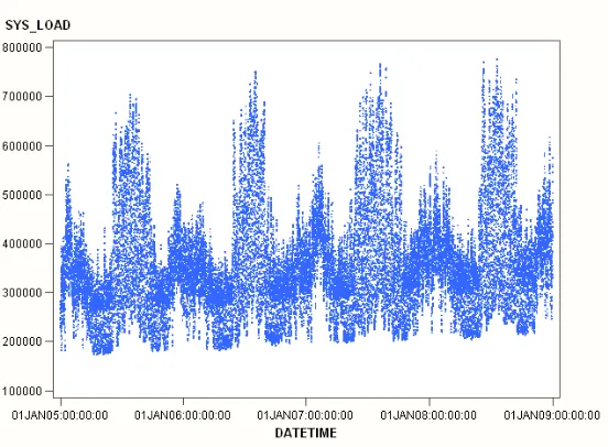
The third set of diagnostic statistics with updating cycle and horizon of one hour, one day, one week, two weeks, and one year described in Section 3.4 is used in the development of the benchmarking model. Figure 4.1 shows the load series from 2005 to 2008, where the following observations can be obtained:

1) Figure 4.1 shows an overall increasing trend year by year. This trend may be due to temperature increase and/or human activities. Since it is hard to draw a conclusion from Figure 4.2 that the temperature has an increasing trend, we can infer that human activities are the major cause of the increasing trend in energy consumption over the years.

(100)

3) Figure 4.1 shows that the summer peak is higher than the winter peak every year, which tells that electricity is primarily used for cooling in the summer. And it also tells that some electricity is used for warming in the winter.

4) Figure 4.1 shows one valley in spring and the other valley in fall every year, which is the result of less need of air conditioning comparing with winter and summer.

(101)

Figure 4.1 Load series (2005-2008).