SCHEFFING, CANDICE CAMILLE. Properties of a Multilayer Coating for Applications in High Level Waste Packaging.* (Under the direction of Dr. Man-Sung Yim and Dr. Mohamed Bourham.)
Materials features that are being considered for the Yucca Mountain high level waste repository include corrosion, hydrogen, and radiation effects as well as structural strength. The current plan for protection of the environment from high level waste placed inside Yucca Mountain includes a defense-in-depth design with multiple engineering barriers. The outer engineered barrier is a large drip shield made of titanium grade-7. Titanium was chosen for its high corrosion resistance and structural strength. This titanium drip shield is an elaborate design that will be expensive and may be susceptible to hydrogen embrittlement or hydrogen-induced cracking. An alternative, multi-layer coating design is proposed that will provide corrosion resistance and act as a barrier to hydrogen diffusion. The coating proposed is composed of the hydrogen barrier titanium nitride (TiN), corrosion resistant zirconium oxide (ZrO2), and wear resistant diamond-like carbide (DLC).
TiN and ZrO2 coatings were deposited on stainless steel substrates using magnetron
sputtering and laser ablation. Analysis of the corrosion resistance of TiN and the multilayer coating, TiN + ZrO2, has been performed at Lawrence Livermore National Laboratory
(LLNL) using simulated waters, representative of the Yucca Mountain environment. The hydrogen barrier properties of TiN have also been analyzed using low temperature resistance measurements and secondary ion mass spectrometry (SIMS) analysis.
Using cyclic polarization testing, TiN was found to be resistant to SCW and BSW, Yucca Mountain simulated waters, with a passive region of 760 ± 342 mV in SCW and 408 ± 67 mV in BSW. The added ZrO2 layer increased the passive region to 822 ± 108 mV in
SCW, and increased the passive region in BSW to 1002 ± 260 mV. The ZrO2 did not
Hydrogen diffusion testing was done on TiN coated stainless steel samples by exposing coated and non-coated samples to hydrogen at an elevated temperature for 3 hours. SIMS analysis indicated that for the TiN-coated samples there was no increase in hydrogen for the exposed sample; rather the hydrogen content of the substrate was lower than the non-exposed sample. The non-coated samples tested in SIMS did not show a difference in hydrogen content between the hydrogen exposed and non-exposed samples. More tests need to be done to confirm claims that TiN is a good diffusion barrier to hydrogen.
The multilayer TiN + ZrO2 coating provides good resistance against corrosion as
shown by the large cyclic polarization passive regions. It does not, however, provide comparable corrosion resistance to titanium, indicating it is not as protective as titanium. The hydrogen barrier property of TiN is an additional property that pure titanium does not have and may be useful for Yucca Mountain. Additional corrosion tests can be done on the ZrO2 coatings to find a more accurate corrosion passive region for the various simulated
Yucca Mountain water. The feasibility of this multi-layer coating will also be an important next step to determine in what ways the coating can be a better choice than titanium as an alternative to the drip shield design at Yucca Mountain.
PROPERTIES OF A MULTILAYER COATING FOR APPLICATIONS IN HIGH LEVEL WASTE PACKAGING
by
CANDICE CAMILLE SCHEFFING
A thesis submitted to the Graduate Faculty of North Carolina State University
in partial fulfillment of the requirements for the Degree of
Master of Science
NUCLEAR ENGINEERING
Raleigh 2005
APPROVED BY:
_______________________________ _______________________________
________________________________ _______________________________
Dedication
Biography
Candice Camille Scheffing grew up in Farmington, New Mexico and became interested in science and engineering at a young age through science fair projects. Her first introduction to Nuclear Engineering was during a science fair project testing for radon in natural gas. She graduated from Farmington High School in 1999 and continued on to college at New Mexico Institute of Mining and Technology in Socorro, New Mexico. She chose to pursue Chemical Engineering and graduated Summa Cum Laude in 2003, earning the Cramer Award for being the top female engineer of her graduating class.
Candice was fortunate to work with an amazing group at Los Alamos National Laboratory for three summers while she was an undergraduate, learning the basics of gamma spectroscopy and becoming familiar with nuclear waste management. She spent the summer after graduation at Oak Ridge National Laboratory doing gamma spectrometry work at the
233
U storage facility. The work she did at ORNL, “Parametric Studies for 233U Gamma Spectrometry,” was recently published in the Journal for Undergraduate Research, v.4 (2004). She went to North Carolina State University in the fall of 2003 and joined the Nuclear Engineering department to begin work on her Masters degree under appointment by the Office of Civilian Radioactive Waste Management to study aspects of high level and spent nuclear fuel waste management. She received a Master of Science degree in Nuclear Engineering in May of 2005 from NCSU.
Acknowledgements
This work would not have been possible without the support provided by the Office of Civilian Radioactive Waste Management. I truly appreciate the opportunities they have given me throughout this research appointment. Colleen Babcock and Norma Ward have been very helpful in making sure that everything concerning the fellowship has run smoothly. My practicum at Lawrence Livermore National Laboratory went beyond my expectations in allowing me to work with many very generous and brilliant people. Special thanks to Dan Day for all his time and patience in explaining potentiostats, corrosion, and geology to me. Also the additional work you did for me after I returned to school has been invaluable. Thanks also to Joseph Farmer, Jeff Haslam, and Lesa Christman for taking me as a student for the summer, despite all the other projects you had going on. I learned so much from all of you and recognize the extra time that you spent to make sure my summer work was a success. Thanks also to Dave Fix for help with the weight-loss samples after their six-months of tank exposure. Other people from LLNL that helped me throughout the summer include Lana Wong, Mike Whalen, John Estill, Ken Evans, Raul Rebak, Tiangan Lian, and Dan McCright. Special thanks to Nancy Yang of Sandia National Laboratories who performed some valuable SEM analysis on my samples.
At NCSU, I would like to thank my advisory committee for meeting with me often and providing support and advice throughout the research process. Thanks to Jag Kasichianula for the use of his lab, equipment, and valuable time to coat many samples for corrosion tests, and even more coatings for hydrogen tests. Thanks to Dr. Bourham for his time and effort in working through EIS theory with me and keeping things simple. Thanks to Dr. Yim for his open door policy and good advice in moving forward in keeping this project active. Thanks also to Dr. Gross for his time in being a part of the committee. Additional people that I cannot forget include April Jackson, Dan Leonard, Mia from the Materials Department, Fred Stevie, and Larry DuFour.
Table of Contents
LIST OF TABLES……….. vii
LIST OF FIGURES……… viii
CHAPTER 1 INTRODUCTION……….. 1
1.1 Background………... 1
1.1.1 Yucca Mountain………..……….. 3
1.1.2 Engineered Barrier Design...……...………. 6
1.1.3 Drip Shield………..……….. 9
1.1.4 Experimental Design……… 11
1.2 Objectives………. 13
CHAPTER 2 COATING………... 14
2.1 Apparatus, Materials, and Methods……….. 15
2.2 Coating Results………. 21
2.3 Discussion………. 25
CHAPTER 3 CORROSION TESTING………... 26
3.1 Apparatus, Materials, and Methods……….. 35
3.1.1 Polarization Testing……….. 35
3.1.2 Weight-loss Testing……….. 39
3.2 Corrosion Testing Results………. 40
3.2.1 Cyclic Polarization Results………... 40
3.2.2 Polarization Resistance Results……… 52
3.2.3 Electrochemical Impedance Results………. 54
3.2.4 Weight-loss Results………... 60
3.2.5 Optical and SEM Images……….. 63
3.3 Discussion………. 67
CHAPTER 4 HYDROGEN DIFFUSION TESTING………. 69
4.1 Apparatus, Materials, and Methods……….. 70
4.2 Hydrogen Testing Results……… 73
4.3 Discussion………. 78
CHAPTER 5 DISCUSSION……….. 80
5.1 Significance of Results………. 80
5.3 Other Applications……… 82
CHAPTER 6 CONCLUSIONS AND FUTURE WORK……… 83
6.1 Conclusions………... 83
6.2 Future Work……….. 84
CHAPTER 7 REFERENCES………... 85
APPENDIX A MATERIAL PROPERTIES……….. 88
APPENDIX B CYCLIC POLARIZATION CURVES………. 89
List of Tables
Table 1.1 Temperature and environment levels for polarization corrosion
testing………... 12
Table 2.1 Coating conditions for mirror polished samples to produce defect-free layers……… 21
Table 3.1 Composition of simulated waters……… 28
Table 3.2 BSW-13 solution recipe (TIP-CM-28, LLNL)……… 29
Table 3.3 Testing solution and temperature for each disk sample………... 38
Table 3.4 Sample ID and position in long-term corrosion SCW vessels………… 40
Table 3.5 Values for plots in Figure 3.29……… 60
Table 3.6 Weight-loss sample data and corrosion rate……… 61
List of Figures
Figure 1.1 Location and disposal schematic for Yucca Mountain HLW repository
(Benton, 2001)………... 4
Figure 1.2 US commercial spent fuel discharge from 1970 – 2020………... 5 Figure 1.3 Defense-in-depth, multiple barrier design concept for repository……… 6 Figure 1.4 a) Engineering barrier design for Yucca Mountain with backfill
(Eckhardt, 2000) and b) without backfill (OCRWM)………... 7 Figure 1.5 Waste package design (Benton, 2001)……….. 8 Figure 1.6 Coating layers and processes under investigation………. 10 Figure 2.1 Disk sample and weight-loss coated with TiN; sample dimensions
indicated……… 16
Figure 2.2 Schematic of magnetron sputtering chamber (Kasichainula)…………... 16 Figure 2.3 Magnetron sputtering chamber front vacuum port showing substrate
bias……… 17
Figure 2.4 Laser ablation vacuum chamber, showing laser beam hitting target at
45o, plume depositing on substrate……… 20 Figure 2.5 SEM image showing de-lamination on coating before electrochemical
testing……… 22
Figure 2.6 SEM elemental analysis shows carbon particle sitting on top of
substrate surface (PEA0994)………. 23 Figure 2.7 400 X optical microscope view of a) smooth TiN surface coated at
400oC and b) rough TiN surface coated at 500oC………. 24 Figure 2.8 X-ray spectrum of TiN coating on silicon-400 substrate……….. 24 Figure 3.1 Pseudo-ternary diagram showing the effect of calcium carbonate and
calcium sulfate precipitation on water composition upon evaporation
(Farmer et. al, 2003)……….. 27 Figure 3.2 a) Controlled potential circuitry using a potentiostat (Jones, 1992), b)
Figure 3.4 Typical polarization resistance curves……….. 32
Figure 3.5 EIS model of sample and equivalent circuit………. 33
Figure 3.6 Equivalent circuit with a) Nyquist plot & b) Bode plot (Jones, 1992)... 34
Figure 3.7 Electrochemical vessel for corrosion testing………. 36
Figure 3.8 Schematic of polarization cell from ASTM standard G5………... 37
Figure 3.9 Titanium nitriding tube furnace block diagram……… 39
Figure 3.10 Selected cyclic polarization curves for 90oC SCW tests………... 41
Figure 3.11 SCW potential comparisons for cyclic polarization corrosion tests……. 42
Figure 3.12 SCW current density comparisons for cyclic polarization corrosion tests……….... 43
Figure 3.13 Cyclic polarization curves for 90oC BSW……… 44
Figure 3.14 BSW potential comparisons for cyclic polarization corrosion tests……. 44
Figure 3.15 BSW current density comparisons for cyclic polarization corrosion tests……… 45
Figure 3.16 Cyclic polarization curves for 5M CaCl2 at 105oC………... 46
Figure 3.17 Cyclic polarization curves for SSW at 90oC………. 46
Figure 3.18 5M CaCl2, SSW potential comparisons for cyclic polarization tests…… 47
Figure 3.19 5M CaCl2, SSW current density comparisons for cyclic polarization tests……….... 47
Figure 3.20 Average potential comparisons for cyclic polarization corrosion tests…. 48 Figure 3.21 Average current density comparisons for cyclic polarization corrosion tests……… 49
Figure 3.22 Matrix of TiN coated samples after corrosion tests showing solution and temperature level of testing……… 50
Figure 3.23 Matrix of TiN + ZrO2 coated samples after corrosion testing showing solution and temperature level of test with zoomed in views of sample surface………... 50
Figure 3.24 Cyclic polarization curves for plain Ti and nitrided Ti in oxalic acid….. 51
Figure 3.26 TiN corrosion rate from polarization resistance tests in 30oC and 60 oC
solutions……… 53
Figure 3.27 Corrosion rates as calculated from polarization resistance tests in high temperature solutions……… 54 Figure 3.28 Equivalent circuit showing current flow, and broken down into solution
resistance and impedance……….. 55 Figure 3.29 RL, Z imaginary from Case II, and the measured impedance, Z, plotted
versus frequency (Hz)……...……… 59 Figure 3.30 Weight-loss samples after removal from corrosion tanks at LLNL (Fix,
2005)………. 62
Figure 3.31 1000X optical a) pre-corrosion and b) post corrosion……….. 63 Figure 3.32 SEM elemental analysis, 2000X post corrosion – dark area indicates
crater where TiN is absent and O is present……….. 64 Figure 3.33 1000X optical a) pre-corrosion and b) post corrosion……...…………... 64 Figure 3.34 SEM image a) 2000X pre-corrosion and b) 1200X post-corrosion…….. 65 Figure 3.35 1000X optical a) pre-corrosion and b) post corrosion……….. 65 Figure 3.36 SEM image a) 1800X pre-corrosion and b) 2000X post-corrosion…….. 66 Figure 3.37 1000X optical a) pre-corrosion and b) post corrosion………...…... 66 Figure 3.38 SEM image a) 3000X pre-corrosion and b) 2000X post-corrosion…….. 67 Figure 4.1 General resistance vs. temperature trend observed between a pure metal
and a metal with impurities………... 70 Figure 4.2 Diagram showing lead location and use on 5 mm-diameter sample for
resistivity measurements………... 71 Figure 4.3 Low temperature hall dewar diagram, 6.0” x 2.5” x 0.75” (MMR
Technologies, 2005)……….. 72 Figure 4.4 Stainless steel resistance vs. temperature data for plain and
hydrogen-exposed………... 74
Figure 4.5 TiN coated resistance vs. temperature data for plain and hydrogen
exposed samples……… 74
Figure 4.7 Nickel and TiN SIMS depth profile for hydrogen exposed and
non-exposed TiN-coated samples………. 76 Figure 4.8 Hydrogen and oxygen SIMS depth profile for hydrogen exposed and
non-exposed TiN-coated samples………. 77 Figure 4.9 Hydrogen, oxygen, and nickel SIMS depth profile for hydrogen
exposed and non-exposed plain stainless steel samples……… 78 Figure B.1 Cyclic polarization curve – TiN coated E316L600, 30 oC SCW……….. 89 Figure B.2 Cyclic polarization curve – TiN coated E316L589, 30 oC SCW……….. 89 Figure B.3 Cyclic polarization curve – plain 316L stainless steel E316L571, 30 oC
SCW……….. 90
Figure B.4 Cyclic polarization curve – TiN coated E316L583, 60 oC SCW……….. 90 Figure B.5 Cyclic polarization curve – TiN coated E316L585, 60 oC SCW……….. 91 Figure B.6 Cyclic polarization curve – TiN coated E316L593, 90 oC SCW……….. 91 Figure B.7 Cyclic polarization curve – TiN coated E316L595, 90 oC SCW……….. 92 Figure B.8 Cyclic polarization curve – plain 316L stainless steel E316L569, 90 oC
SCW……….. 92
Figure B.9 Cyclic polarization curve – TiN/ZrO2 coated E316L001, 90 oC SCW…. 93
Figure B.10 Cyclic polarization curve – TiN/ZrO2 coated E316L009, 90 oC SCW…. 93
Figure B.11 Cyclic polarization curve – TiN/Ti/TiN coated PEA0991, 90 oC SCW... 94 Figure B.12 Cyclic polarization curve – TiN/TiN (laser) coated PEA0992, 90 oC
SCW……….. 94
Figure B.13 Cyclic polarization curve – TiN/TiN/TiN coated PEA0993, 90 oC
SCW……….. 95
Figure B.14 Cyclic polarization curve – TiNTi/Ti coated PEA0994, 90 oC SCW…... 95 Figure B.15 Cyclic polarization curve – TiN coated E316L591, 30 oC BSW……….. 96 Figure B.16 Cyclic polarization curve – TiN coated E316L599, 30 oC BSW……….. 96 Figure B.17 Cyclic polarization curve – TiN coated E316L586, 90 oC BSW……….. 97 Figure B.18 Cyclic polarization curve – TiN coated E316L594, 90 oC BSW……….. 97 Figure B.19 Cyclic polarization curve – TiN/ZrO2 coated E316L002, 90 oC BSW…. 98
Figure B.20 Cyclic polarization curve – TiN/ZrO2 coated E316L003, 90 oC BSW…. 98
Figure B.22 Cyclic polarization curve – TiN coated E316L596, 90 oC SSW……….. 99
Figure B.23 Cyclic polarization curve – Plain 316L stainless steel E316L570, 90 oC SSW………... 100
Figure B.24 Cyclic polarization curve – TiN/ZrO2 coated E316L005, 90 oC SSW…. 100 Figure B.25 Cyclic polarization curve - TiN coated E316L581, 30 oC 5M CaCl2... 101
Figure B.26 Cyclic polarization curve - TiN coated E316L584, 105 oC 5M CaCl2…. 101 Figure B.27 Cyclic polarization curve – TiN/ZrO2 coated E316L004, 105 oC 5M CaCl2………. 102
Figure C.1 TiN coated E316L582 disk sample before test………. 103
Figure C.2 TiN/ZrO2 coated E316L009 disk sample before test……… 103
Figure C.3 TiN coated weight-loss sample before test………... 103
Figure C.4 TiN coated E316L581 after polarization test in 5 M CaCl2 at 30oC……. 104
Figure C.5 TiN coated E316L584 after polarization test in 5 M CaCl2 at 105oC…... 104
Figure C.6 TiN coated E316L588 after polarization test in SSW at 90oC………….. 104
Figure C.7 TiN coated E316L591 after polarization test in BSW at 30oC…………. 105
Figure C.8 TiN coated E316L599 after polarization test in BSW at 30oC…………. 105
Figure C.9 TiN coated E316L586 after polarization test in BSW at 90oC…………. 105
Figure C.10 TiN coated E316L594 after polarization test in BSW at 90oC…………. 106
Figure C.11 TiN coated E316L589 after polarization test in SCW at 30oC…………. 106
Figure C.12 TiN coated E316L600 after polarization test in SCW at 30oC…………. 106
Figure C.13 TiN coated E316L583 after polarization test in SCW at 60oC…………. 107
Figure C.14 TiN coated E316L585 after polarization test in SCW at 60oC…………. 107
Figure C.15 TiN coated E316L593 after polarization test in SCW at 90oC…………. 107
Figure C.16 TiN coated E316L595 after polarization test in SCW at 90oC…………. 108
Figure C.17 TiN/ZrO2 coated E316L004 after polarization test in 5M CaCl2 at 105oC………. 108
Figure C.18 TiN/ZrO2 coated E316L005 after polarization test in SSW at 90oC……. 108
Figure C.19 TiN/ZrO2 coated E316L002 after polarization test in BSW at 90oC…… 109
Figure C.20 TiN/ZrO2 coated E316L003 after polarization test in BSW at 90oC…… 109
Figure C.21 TiN/ZrO2 coated E316L001 after polarization test in SCW at 90oC…… 109
Figure C.23 TiN coated weight-loss samples W316L581-583 after 6-month
exposure in 90oC SCW Vapor………... 110 Figure C.24 TiN coated weight-loss samples W316L590-592 after 6-month
exposure in 60oC SCW Vapor………... 111 Figure C.25 TiN coated weight-loss samples W316L587-589 after 6-month
exposure in 90oC SCW aqueous………... 111 Figure C.26 TiN coated weight-loss samples W316L584-586 after 6-month
exposure in 60oC SCW aqueous………... 112 Figure C.27 TiN coated weight-loss samples W316L594-595 after 6-month
exposure in 90oC SCW at water line………. 112 Figure C.28 TiN coated weight-loss sample W316L593 after 6-month exposure in
Chapter 1
INTRODUCTION
1.1 Historical Background on Spent Nuclear Fuel and High Level Waste
The United States is currently faced with a large-scale storage/disposal dilemma for the highly radioactive materials produced from civilian nuclear power operations, defense nuclear programs, and smaller-scale industrial and institutional research and health activities. These materials include spent nuclear fuel (SNF) that has been irradiated in a nuclear reactor and withdrawn because it has decreased in useful enrichment, high level waste (HLW) which comes from reprocessing of SNF from either defense or civilian origin, transuranic waste (TRU) which includes any alpha emitting isotope with an atomic number greater than 92, half-life longer than 20 years and a concentration greater than 3.7 x 10⁶ Bq/kg (100 nCi/g waste), and low-level waste (LLW) which includes any waste other than SNF, HLW, or TRU. LLW is regulated by the Department of Transportation and the Nuclear Regulatory Commission but handled and disposed by states and regions. Commercial LLW is sent to one of three disposal facilities found in South Carolina, Washington, or Utah (Saling, 2002). Solid TRU waste is currently being disposed of at the Waste Isolation Pilot Plant in Carlsbad, New Mexico, shipped from all over the country.
storage sites at individual reactor sites (Murray, 2003). However, these spent fuel pools and dry storage areas are not meant to be the final disposal location of the nuclear reactor by-product.
Spent fuel from commercial energy producers is destined for a final deep geological disposal by the Federal Government’s Department of Energy (DOE). In 1982 the Nuclear Waste Policy Act (NWPA) was passed by Congress, which was a compromise among industry, government, and environmentalists outlining the timeline for the DOE to ultimately dispose of HLW/SNF geologically (from this point forward, SNF will be combined into the term HLW unless specifically addressing aspects of SNF). Since the NWPA was passed, power generators have been charging a fee of one-tenth of a cent for each kilowatt-hour to help DOE pay for the research and development of a site for disposal. Also, as a result of the NWPA, a new office for addressing this task was set up in the DOE, the Office of Civilian Radioactive Waste Management (OCRWM). This office started out by studying various locations as possible sites for the geological HLW disposal. The site possibilities were narrowed down to three by 1987, including Deaf Smith County, Texas, Hanford, Washington, and Yucca Mountain, Nevada. At this time, Congress amended the NWPA, which declared Yucca Mountain as the only site that would be further investigated by DOE for geological disposal. Since 1987, the OCRWM has been characterizing and studying aspects of HLW disposal at Yucca Mountain including geology, hydrology, seismology, volcanology, meteorology, ecology, as well as social aspects such as law, sociology, demography, and politics.
not anticipate waste acceptance until 2010. In the aftermath of the September 11 terrorist attacks, national security has become a major argument for opening a repository at Yucca Mountain (Zacha, 2002). It has become more important to remove the many scattered targets around the country and safely dispose of all HLW in an underground repository. It has again come up in recent news that the demand for some form of HLW sequestration needs to be addressed due to the current obstacles and delays to certifying, licensing, and opening the Yucca Mountain Repository. The National Commission on Energy Policy has suggested the opening of two independent spent fuel storage installations (ISFSI) to be built (Tompkins, 2005), thus reducing the number of dry-cask storage areas from roughly 100 to 2.
The pressure for opening the Yucca Mountain Repository is great, and there are many factors that will influence how quickly this project moves forward. The research for this thesis is based on the assumption that Yucca Mountain will be opening in the future and that the engineered barrier design can be improved upon, particularly in regards to cost with possible improvements in performance.
1.1.1 Yucca Mountain
Yucca Mountain has been studied since 1978 by the DOE to determine if it is suitable for the nation’s first long-term geologic repository for SNF and HLW (OCRWM, 2004). The ultimate purpose of the characterization has been to understand the mountain’s physical aspects and the processes that could affect the mountain’s safety. Safety to the public and to the environment over the next 10,000 years is being estimated/predicted using the results of the thousands of studies that have been carried out at multiple universities and national laboratories. The natural ability of the repository site is of great interest to ensure isolation of the waste and to minimize the amount of radioactive material that can migrate from the facility. The design of the repository includes a series of excavated tunnels, or drifts, deep underground in the solid rock of Yucca Mountain. The layout of the drifts was made to manage the heat that would be produced by the SNF (OCRWM).
1,500 m to 1,930 m above sea level, an irregularly shaped volcanic upland. It is located in a region known as the Great Basin, composed of volcanic tuff formed when lava having mineral gas content welded with ash into a dense, non-porous rock approximately 11.5 to 14 million years ago. The volcanoes that formed this region have been extinct for
Figure 1.1 Location and disposal schematic for Yucca Mountain HLW repository (Benton, 2001).
approximately 20 km (14 mi) south of Yucca Mountain (Wilson et. al., 2002). The mean annual temperature at Yucca Mountain is 63o Fahrenheit. There are no known natural resources of value such as precious metals, mineral, or oil located at the site. In addition to low rainfall and no natural resources in the area, the very location of Yucca Mountain near the Nevada Test Site makes it an ideal location because of the contamination from nuclear tests that occurred there.
As described in the NWPA, Yucca Mountain has a capacity of approximately 70,000 metric tons of uranium (MTU). This volume will account for the amount of SNF that is currently being stored at reactors across the country. With the reactor license extensions that are occurring, however, it is easy to predict that 70,000 MTU will not be sufficient for disposing of all the country’s SNF. Figure 1.2 shows the cumulative U.S. commercial spent fuel discharges from 1970 thru 2020 (Murray, 2003).
Yucca Mountain Capacity
Figure 1.2 US commercial spent fuel discharge from 1970 – 2020.
likelihood of future volcanic disruption is minimal (Benton, 2001). Uncertainties that are present in the characterization studies due to the length of time that is being predicted (10,000 years) are high. In response to this, the design for the Yucca Mountain Repository has been made as a defense-in-depth design, which not only includes the natural barriers of the Mountain, but also includes robust engineering designs to help in achieving the repository’s objectives.
1.1.2 Engineered Barrier Design
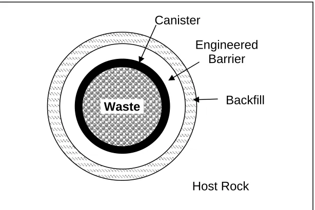
Federal regulations require that the repository for nuclear waste include at least one natural barrier and one engineered barrier to protect against water reaching the waste, degrading it, and transporting radioactive particles (NRC, 2001). The combination of the mountain’s natural features and technology-based engineered components supports the defense-in-depth approach, which is illustrated in Figure 1.3.
Canister
Engineered Barrier
Backfill
Waste
Host Rock
Figure 1.3 Defense-in-depth, multiple barrier design concept for repository.
uranium oxide in zircaloy cladding, vitrified glass, or HLW mixed with cement. The second barrier is the canister or waste package in which the waste form is placed; typically, it is a large metal container that can hold multiple wastes in one bundle. The engineered barrier is an additional man-made barrier in a repository drift that adds even more protection in addition to the waste package and waste form. This diagram also indicates backfill, which is the host rock that was removed to drill the shafts and/or a highly sorbent material that can be placed into the drift around the waste package. The backfill acts as a liquid absorber and helps sorb moisture away from the waste. The host rock is the natural barrier for the design.
This concept has gone through several different design iterations over the past few years, with different designs having different types and forms of barriers that could account for the multiple-barriers. As examples, Figure 1.4a shows a design with a backfill, and Figure 1.4b shows the design without a backfill. The current design for Yucca Mountain, as seen in Figure 1.4b, does not include a backfill. This may be due to the fact that there is not expected to be a lot of seepage into the disposal drifts that would need to be diverted away from the waste package. The drip shield will likely be sufficient for seepage/drip diversion.
a b
Figure 1.4 a) Engineering barrier design for Yucca Mountain with backfill (Eckhardt, 2000) and b) without backfill (OCRWM).
is known from the design of reactor fuel for the corrosive environments inside reactors. The waste form should hold the waste for several hundred years during which most of the radionuclides decay to safe levels (Murray, 2003).
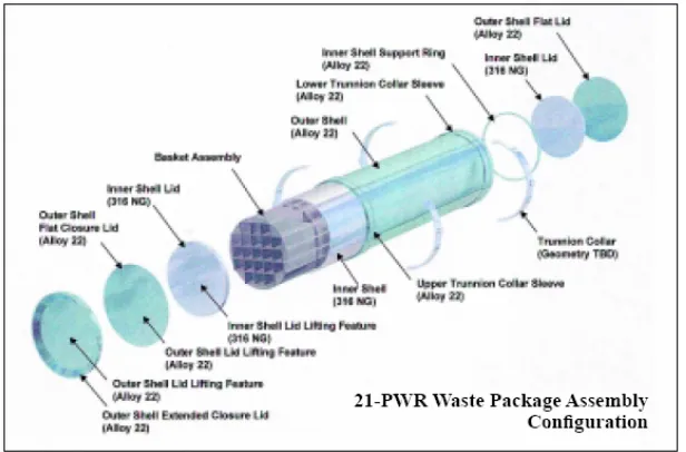
The waste package has gone through several different designs, while the current model is that of two thick metal cylinders, one nested within the other. This design is meant to withstand many different environments especially those involving different corrosive activity. The inner shell would be made of stainless steel 316 Nuclear Grade (NG) which will improve the waste package’s performance because it is less susceptible to oxidation than carbon steel. The outer shell will be made of Alloy 22, a nickel-based alloy that has proven to be highly resistant to corrosion (Benton, 2001). Figure 1.5 is a diagram of this cylinder within a cylinder design for the waste package at Yucca Mountain.
Figure 1.5 Waste package design (Benton, 2001).
(OCRWM). The drip shield was the motivation for this thesis work and will be discussed in more detail in the next section.
The host rock of Yucca Mountain is the largest and most effective barrier in the entire design. The geologic processes that occur in and around Yucca Mountain act to filter and delay particles from first, reaching the emplacement drifts, and further being transported into the water table. The migration of radioactive material through the geologic area of Yucca Mountain will be low because of surfaces within the rock such as particles, pores, grain boundaries, and fissures which all generally have a retarding effect on the motion of groundwater and waste material (Burkholder, 1980).
1.1.3 Drip Shield: Important Issues to Consider
The titanium drip shield mentioned in the previous section is a large shield meant to divert any liquid water seepage from the host rock, around the waste packages, and onto the drift invert. It will be emplaced in segments that link together, forming a single, continuous barrier for the entire length of each emplacement drift (OCRWM, 2000). The main design requirements for the drip shield are corrosion resistance and structural strength. The corrosion resistance is meant to ensure high performance reliability for 10,000 years. The structural strength is meant to protect the waste package from damage due to rock fall. The bulk of the drip shield will be made from titanium grade 7 at a thickness of 15 mm (0.6 in).
absorbed by the titanium drip shield which could cause hydrogen embrittlement and/or hydrogen induced cracking.
As a proposal for a possible alternative to this titanium drip shield, the work for this thesis has investigated the properties of a multilayer coating design that could provide good corrosion resistance as well as prevent the absorption of hydrogen into an underlying metal. The possibilities of using a different material for a drip shield should take into account many aspects of the project including material properties (corrosion, structural strength, and hydrogen absorption/diffusion), economics, and application possibilities. For this study, the main properties considered are corrosion and hydrogen susceptibility, as could be studied in a laboratory setting. Structural integrity, application possibilities, and economics are considered briefly but not studied in depth.
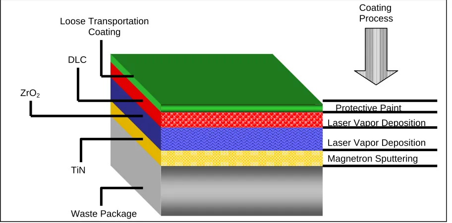
The proposed alternative is a series of coatings that can be applied as multi-layers to provide a diffusion barrier to hydrogen, wear and erosion protection, corrosion and radiation resistance, and strong adhesion. The coatings were determined based on their individual properties that matched those that were important for this type of multi-layer coating. The overall design has three coated layers of titanium nitride (TiN), zirconium oxide (ZrO2), and diamond-like carbide (DLC) under a final protective paint coating.
The coating layers and process for coating application can be seen in Figure 1.6.
Coating Process
Figure 1.6 Coating layers and processes under investigation.
ZrO2
Loose Transportation Coating
DLC
Protective Paint
Laser Vapor Deposition
Laser Vapor Deposition
Magnetron Sputtering TiN
TiN has been shown to lower hydrogen permeability by at least four orders of magnitude (Checcheto et. al., 1996). This layer also has good adhesion properties and stability on titanium alloy substrates. TiN can be deposited using magnetron sputtering, utilizing a titanium target and nitrogen gas to produce plasma, combining atoms of Ti and N to form a near stoichiometric thin film of TiN.
The second coated layer of ZrO2 is proposed for its protective properties against
corrosion and its high wear resistance. Zirconium is insoluble in water and is resistant to high levels of radiation as observed in its uses in nuclear reactors as a fuel cladding material. ZrO2 is also known to have good thermal barrier properties. The third coated
layer, DLC, is proposed for its uses as hard, wear resistant tools, and for its lubricating properties (Voevodin et. al., 1995). This top layer is thought to add strength properties to the coating, but its adhesion properties may be problematic. The coating method proposed for both the ZrO2 and DLC coatings is laser ablation. The coating processes are
described in more detail in Chapter 2 where the coatings are produced and results are presented.
The majority of characterization work done for this multi-layer coating was done at Lawrence Livermore National Laboratory (LLNL) using their advance corrosion facility. Corrosion testing involved polarization tests on small 316L stainless steel disk samples coated with TiN and weight-loss testing on 316L stainless steel weight-loss samples. Additional characterization was performed on samples using optical and SEM microscopy of the coatings. TiN was also tested for its ability to prevent hydrogen from diffusing through into the underlying substrate. This was tested using low temperature resistance measurements and secondary ion mass spectroscopy (SIMS) analysis.
1.1.4 Experimental Design
to three day turnaround from start to finish for each test, utilizing two polarization cells for testing. Coating of samples also required about two and a half to three days because of the time needed to reach a good vacuum, raise the temperature, and decrease the temperature at a controlled rate. Samples that were corrosion tested using polarization (disk samples) required only one side to be coated while the weight-loss samples required all sides to be coated.
Taking the time and materials available for coatings, the corrosion tests were planned to allow for multiple tests at each environment/temperature level. Initially, there were a total of three temperature levels and four environments to be tested. Table 1.1 indicates the generic temperature and environment levels needed for complete testing in possible Yucca Mountain conditions.
Table 1.1 Temperature and environment levels for polarization corrosion testing. Environment and temperature levels are described in Chapter 3.
Temperature 1 Temperature 2 Temperature 3
Environment 1 XX XX XX
Environment 2 XX XX
Environment 3 XX
Environment 4 X X
Twelve samples would be needed for one test at each level and twenty four samples for two tests at each level. A more desirable number of replicates is three at each level (36 samples total), but with a total of twenty stainless steel samples available for coating, it would not even be possible to test each level twice. It would also be difficult to perform this many polarization tests in the short 12 weeks available at LLNL. In order to prepare for these shortcomings, more stainless steel samples were cut, polished, and coated at NCSU before heading to California for corrosion testing, and the most important temperature and environment levels were determined.
were done on TiN-coated samples with an X for each test performed at the corresponding environment and temperature level. Only six samples were coated with the multilayer of TiN + ZrO2, which required careful testing. Samples that were coated with multiple
layers were tested at the high temperature levels for each environment, in order to test at the more corrosive level (higher T = higher corrosion rate). In the end, a total of 28 samples were tested, 15 with a TiN coating, 3 plain stainless steel samples, and 6 that were coated with TiN and ZrO2. The last 4 were coated with multiple layers of TiN and
tested in the high temperature level of the most likely environment (Environment 1). The tanks for testing the weight-loss samples had two temperatures and one environment with three positions (vapor, waterline, or submerged) available for testing. These samples also took much longer to coat with TiN using magnetron sputtering (2 per week). Only 15 weight-loss samples were completely coated, and these were divided evenly among the temperature and environment positions, depending on the space available in the tanks. The final testing condition for both the disk and weight-loss samples is described in Chapter 3.
1.2 Objectives
As indicated in sections 1.1.3 and 1.1.4, the main objective for this thesis is to produce coatings of TiN, TiN + ZrO2, and TiN + ZrO2 + DLC and test their corrosion
Chapter 2
COATING
The coatings that were applied during the course of this thesis work include titanium nitride (TiN), zirconium oxide (ZrO2), and diamond-like carbon (DLC). The two deposition
methods used were magnetron sputtering and laser ablation. The majority (~85%) of the completed coatings were TiN deposited using magnetron sputtering. The discussion in this section includes, first, how magnetron sputtering and laser ablation are performed, then describes the apparatus and procedure specific to these coatings. The final section presents the results and the quality of the coatings applied.
In the magnetron sputtering process, plasma is generated using a pulsed DC voltage applied between two electrodes. Ions are accelerated by the sheath potential and impact on the target (sputtering material), where the sputtered ions are allowed to deposit onto the surface of the substrate and form the desired deposited layer. The magnetic field is used to trap electrons and allow only ions to reach the target surface. The coating layer can be altered by changing the target material or changing the gaseous ions introduced into the chamber. For example, to produce a titanium coating, argon gas with a titanium target is used. The ions produce blue plasma that sputters titanium but does not combine with the metal. To produce TiN, nitrogen gas is introduced along with argon. The resulting pink plasma nitrogen ions combine with the sputtered titanium ions to produce TiN.
The second and third layers in the coating model, zirconium oxide (ZrO2) and
diamond-like carbide (DLC), were produced using pulsed laser ablation rather than magnetron sputtering. This was done due to target availability for ZrO2 and DLC, and better
ablation to minimize any chemical reaction products and encourage crystalline film growth. The substrate was positioned so that the plume could condense onto it, forming a thin film. There are many parameters that need to be considered for efficient laser ablation including the pulse duration and energy, laser power, focal length and target distance, and the beam quality.
2.1 Apparatus, Materials, and Methods
Initial preparations included the cleaning and polishing of the substrates. Several deposition conditions were attempted with different substrate materials to find the ideal coating conditions for improvement in the corrosion resistance. Early depositions of the coatings were on carbon steel samples, 1.5” x 0.25” x 0.125” (38.1mm x 6.35mm x 3.175mm), that were polished down to a 600 grit finish on all sides. The carbon steel samples were cleaned in soapy de-ionized water, rinsed, and etched with 70% phosphoric acid. Thoroughly dried samples were stored until ready for coating. Prior to deposition of the films, the samples were cleaned with alcohol followed by acetone. It was discovered that the etching process did not allow for the coating to adhere to the sample. The substrates were polished again with 600 grit polishing paper and cleaned with water followed by alcohol and acetone. This removed the poor coating and began the procedure again while neglecting the etching process. The carbon steel samples were not the correct dimensions to perform corrosion tests at LLNL, but were a useful starting point to find optimal coating parameters (deposition temperature and current from power supply).
the disk sample and the weight-loss sample with the orange-gold coloring from the TiN coating.
51 mm
16 mm
Disk sample
26 mm
Weight-loss sample
Figure 2.1 Disk and weight-loss samples coated with TiN; sample dimensions indicated.
The magnetron sputtering chamber consisted of a vacuum chamber (8 – inch diameter), vacuum gauges (Phillips series 275 conductance gauge, Granville-Phillips series 270 high-vacuum ion gauge), argon and nitrogen gas supply, 4 – inch diameter titanium target, and power supply (DORA Power System, MSS-10, 3x208V). A schematic of the magnetron sputter chamber is shown in Figure 2.2.
The substrate holder is a stage for the substrate to be placed inside the chamber, made of a hollow ceramic that has coiled tungsten wire inside for heating. There is also a shutter that moves from a ‘closed’ position covering the substrate to an ‘open’ position without affecting the vacuum or other operating procedures. The shutter was used to avoid deposition on the substrate during cleaning of the target. The chamber was cooled by coiled copper around the target area with chilled water flowing through from an in-room water chiller (Neslab Coolflow Refrigerated Recirculator, HX-150). A photo of the chamber vacuum port can be seen in Figure 2.3.
Figure 2.3 Magnetron sputtering chamber front vacuum port showing substrate bias.
minute. Once the temperature reached approximately 350 oC, the pulsed DC supply was connected to the target, including a ground connection, and the temperature was raised to 500
o
C at a rate of 8 oC per minute. With the increase in temperature, the pressure in the chamber increased slightly to approximately 10-5 Torr. After the power supply was safely connected and the temperature was at 480 – 520 oC, argon gas (99.999% UHP) was introduced into the chamber at a pressure of 2 mTorr.
With Argon gas flowing into the chamber, the power supply was turned on for a timed ‘cleaning’ of 3 minutes while the shutter still covered the substrate from bombarding ions. The soft blue plasma, formed after turning the power supply on, was maintained with a current level set at 0.50 - 0.70 amps (A). Typically, this level of current corresponded to an effective power of 0.25 – 0.35 kW and a circulating power of 0.17 - 0.21 kW. After three minutes, cleaning was completed; with the argon gas still flowing at a pressure of 2 mTorr, the power supply was turned on again and nitrogen gas (99.999% UHP) was introduced into the chamber at a pressure of 2 mTorr. The Nitrogen gas produced soft pink plasma and the current was raised to a higher level for deposition. This pink-colored plasma indicated the formation of titanium nitride, and the current was increased to a level of about 1.48 - 1.52 A (0.73 – 0.75 kW effective power, 0.51 – 0.56 kW circulating power). The shutter was then moved so that it no longer covered the substrate, and these deposition conditions were held for 45 minutes. These conditions were known previously to produce approximately a 0.5 – 1.0 µm layer of coating, where approximately 2 – 3 Angstroms of the film per second were deposited (1 µm / 10,000 Å; 2700s*(2 to 3) = 5400Å to 8100 Å = 0.54 µm to 0.81 µm).
At the end of the 45 minute deposition, the power supply was turned off and disconnected, temperature was reduced at a rate of about 5 – 10 oC per minute, and the argon gas pressure was discontinued. Nitrogen pressure was reduced only slightly so as to provide a positive pressure of nitrogen purge as the sample was cooled to room temperature. After the sample was completely cooled, the chamber was purged with nitrogen and the vacuum turned off to allow it to reach atmospheric pressure. The chamber was then opened and the sample removed for further characterization.
sides. All these samples were characterized at LLNL for corrosion resistance as described in Chapter 3. Additional coatings using the magnetron sputtering method were performed on small test samples of stainless steel 304 for hydrogen analysis per description in Chapter 4. These test samples were circular disks with a 5 mm diameter and a thickness of 1 mm. These samples were polished on both sides with 600 grit paper and 5 µm alumina abrasive followed by cleaning with de-ionized (DI) water and ultrasonically cleaned in alcohol. The coatings were performed at different temperatures (between 400oC and 500oC) to determine the effect of substrate temperature on the coating smoothness and quality.
The TiN, ZrO2, and DLC multilayer coatings were deposited using an Nd-Yag laser
in the 4th harmonic (Spectra Physics Quanta Ray, GCR – 270) with 226 nm wavelength and 10 Hz pulse frequency. The pulse duration is 8-9 nano-seconds with the pulse energy of 210 mJ/pulse. The beam was focused onto the target using a focusing lens. The targets, TiN, ZrO2 (Cerac, Yttria stabilized 1 – inch diameter), and carbon, were placed on a rotating target
stage for a 45o laser incidence. The substrate was held parallel and approximately 3 centimeters from the target so that the plume is deposited directly onto the surface. The target and substrate were inside a vacuum chamber that reached 10-7 Torr prior to deposition. A schematic of the laser ablation system used is shown in Figure 2.4. The deposition chamber was baked using a resistance heater to remove water vapor and oxygen in the chamber. The substrate was finally heated to 400oC for deposition of the films. The deposition rate was approximately 1 – 2 Å per pulse. The deposition of the TiN/ZrO2
multilayer structure was performed for 30 minutes for each layer. Multilayer deposition of TiN/ZrO2/DLC was performed for 30 minutes, each for TiN and ZrO2 and 15 minutes for
Figure 2.4 Laser ablation vacuum chamber, showing laser beam hitting target at 45o, plume depositing on substrate.
Vacuum
Chamber
Port
Target Multiple Target
holder
Laser Beam
Plume
Rotatable substrate holder
Port Port
Four samples with both TiN + ZrO2 coatings and two samples with all three layers,
TiN + ZrO2 + DLC, were made due to limited substrates and time constraints. TiN, ZrO2 and
carbon targets were placed on a rotating target stage for the laser ablation of coatings that allowed for an in-situ sequential deposition of each layer without introducing contamination to the surface between different coating layers. The samples that were coated with multiple layers were prepared entirely in the laser deposition system.
Table 2.1 – Coating conditions for mirror polished samples to produce defect-free layers.
Sample Coating Method Coating Layers
Bottom/middle/ top Temperature Current
PEA 0991 Mag. Sputtering TiN / Ti / TiN 500 oC 2 A
PEA 0992 Laser Ablation TiN / TiN 450 oC n/a
PEA 0993 Mag. Sputtering TiN / TiN / TiN 500 oC 2 A
PEA 0994 Mag. Sputtering TiN / Ti / Ti 500 / 400 oC 1.5 A
These samples were characterized using a scanning electron microscope (SEM) with elemental mapping capabilities before and after corrosion testing.
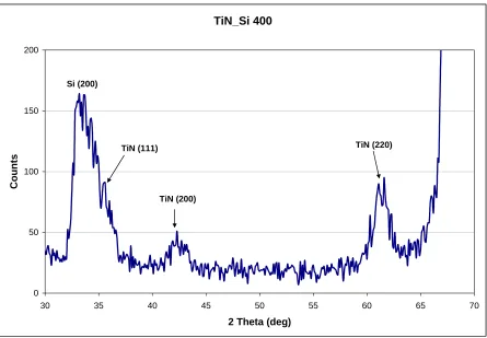
X-ray diffraction was used to determine the crystallinity of the TiN film. A TiN film on silicon (400) substrate was characterized using the x-ray diffractometer. because the film on the stainless steel contained extra peaks that shadowed the TiN lines. A Rigaku Geigerflex model number 58741 diffractometer with Cu Kα (1.5404 Å) was operated at 27.5 kV and 22 mA with a slit width of 2o for x-ray work.
2.2 Coating Results
Polished samples of carbon-steel were difficult to coat without defects and delaminated areas of coating that were visible in an optical microscope at 1000X. Multiple coatings on top of each other were often needed on the carbon steel to produce a uniform coating to the scale as seen through an optical microscope. The initial coatings, completed on carbon steel for the first test of coating application requirements, led to the final procedure used for the remaining sample coatings of TiN using magnetron sputtering.
The corrosion testing required samples of specific dimensions, and therefore coatings were prepared on 316L stainless steel disk and weight-loss samples shown in Figure 2.1. Coatings on these samples were not as prone to defects and delaminated areas. The first set of samples of stainless steel that were coated produced smooth, yellow-gold colored coatings of TiN. The polished disk samples, as viewed through an optical microscope, were continuously coated and there were no obvious defects visible.
(produced by Nancy Yang at Sandia National Laboratories). While this figure shows the SEM image of only one sample, E316L-598, it cannot be ruled out that this phenomenon is not seen on other samples. The disk samples were coated with TiN in batches of eight using magnetron sputtering.
Figure 2.5 SEM image showing de-lamination on coating before electrochemical testing.
Figure 2.6 SEM elemental analysis shows carbon particle sitting on top of substrate surface (PEA0994).
a b Figure 2.7 400 X optical microscope view of a) smooth TiN surface coated at 400oC and b) rough TiN surface coated at 500oC.
The x-ray diffraction peaks are shown in Figure 2.8, with the silicon (200) forbidden peak on the far left and silicon (400) peak on the far right of the spectrum. TiN gives peaks at 2-theta values of 36.67o for the (111), 42.6o for the (200), and 61.82o for the (220) reflections. All of these peaks are observed in Figure 2.8, with the (111) peak distorted by
TiN_Si 400
0 50 100 150 200
30 35 40 45 50 55 60 65 70
2 Theta (deg)
Count
s
Si (200)
TiN (111)
TiN (200)
TiN (220)
the large silicon (200) peak. This x-ray diffraction spectrum indicates that the coating formed using magnetron sputtering is a good layer of TiN.
2.3 Discussion
The coating process using magnetron sputtering for TiN went through several different variations in the substrate deposition temperature and the deposition current used. Based on the optical and SEM images it appears that a single coating has a susceptibility to surface defects which could cause a decrease in its protective properties. The adhesion of the coating was affected by the surface conditions and preparation prior to coating as well as by the actual substrate material. TiN did not adhere well to carbon steel, but did adhere to 316L stainless steel. An added layer of titanium coated on the substrate before coating the TiN increased the adhesion. The deposition temperature that produced a smooth coating was 400
o
C along with a current source of 2 A. A higher deposition temperature produced a rougher surface, but still produced a good, continuous coated layer. The x-ray analysis performed showed that the coating produced was crystalline TiN without added impurities.
The laser deposition process produced an effective coating of ZrO2, but it was
difficult to produce a good DLC layer. The DLC did not adhere well to the ZrO2 layer.
Chapter 3
CORROSION TESTING
All testing for corrosion resistance was completed at Lawrence Livermore National Laboratory (LLNL) in Livermore, California during the summer months of 2004. Electrochemical corrosion testing has been done for many years, and for the specific case of corrosion at Yucca Mountain there has been considerable research into precise environments that may be present in the disposal drifts and cause corrosion (OCRWM, 2002). The facility at LLNL has been involved in the Yucca Mountain project since 1977, and has been doing the most extensive corrosion testing for the project. It is home of the Long Term Corrosion Test Facility (LTCTF) where many important materials corrosion studies have been and currently are being done to help with the characterization and design for the project.
2 Ca + 2 4 SO − 2- -4 3
Ca > SO + HCO
2 4 3 Ca<SO−+HCO−
3
Ca<HCO−
3
HCO−
Ca-Chloride Brine (Na-K-Ca-Mg-Cl-NO3) Sulfate Brine (Na-K-Mg-Cl-SO4-NO3)
Na-Bicarbonate Brine (Na-K-CO3-Cl-SO4-NO3)
Equivalent Percent (%)
Figure 3.1 Pseudo-ternary diagram showing the effect of calcium carbonate and calcium sulfate precipitation on water composition upon evaporation (Farmer et. al, 2003).
There are several different simulated waters that have been made to represent the waters predicted by the evaporation model. These waters include:
• Simulated concentrated water (SCW) – concentrated J-13 well water, bicarbonate
• Simulated dilute water (SDW) – less concentrated J-13 well water, bicarbonate
• Basic saturated water (BSW) – saturated bicarbonate with basic pH
• Simulated acidified water (SAW) – concentrated sulfate with acidic pH
• Saturated sulfate water (SSW) – saturated sulfate
• Concentrated calcium chloride (5 M CaCl2) – calcium solution.
All of these waters are based on analyses of J-13 well water, which is a representative water well near Yucca Mountain. It is a dilute sodium – bicarbonate – carbonate (Na-HCO3-CO3)
water, and the simulated concentrated water (SCW) is 1000 times the concentration of this well water. SDW is 10 times more concentrated than J-13 well water, while SAW is 1000 time more concentrated, and acidified using sulfuric acid (H2SO4). SSW is based upon a
separate assumption that the evaporation of J-13 well water becomes a sodium – potassium – chloride – nitrate solution with the absence of sulfate and carbonate. This water is a concentrated solution that begins to solidify at temperatures below 90oC. BSW is a test environment that has a pH between 11 and 13 and a boiling point near 110oC. The solution for BSW has three separate recipes depending on the desired pH level. The CaCl2 solution is
considered the harshest environment for Yucca Mountain, but at the same time is unlikely. Recent analysis by the NWTRB has concluded that this environment is in fact unlikely to occur and cause significant corrosion to the Alloy 22 waste package (NWTRB, 2004). Of the remaining solutions from those listed, a bicarbonate solution is the most likely with BSW being the most aggressive environment in that set. The compositions for SCW, SDW, SAW, and SSW can be seen in Table 3.1, while the recipe for BSW-13 is given in Table 3.2.
Table 3.1 Composition of simulated waters.
Concentration (mg/L)
Ion SCW SDW SAW SSW
K+ 3400 34 3400 141,600
Na+1 40,900 409 37,690 487,000
Mg+2 <1 1 1000 0
Ca+2 <1 0.5 1000 0
F-1 1400 14 0 0
Cl-1 6700 67 24,250 128,400
NO3-1 6400 64 23,000 1,310,000
SO4-2 16,700 167 38,600 0
HCO3-1 70,000 947 0 0
Table 3.2 BSW-13 solution recipe (TIP-CM-28, LLNL) Chemcal Chemical Quantity
KCl 8.7 g
NaCl 7.9 g
NaF 0.2 g
NaNO3 13.0 g
Na2SO4 1.4 g
H2O (deionized) 66 ml
10N NaOH 2 ml
pH 13.13
a b Figure 3.2 a) Controlled potential circuitry using a potentiostat (Jones, 1992), b) Pathway of a general electrode reaction (Bard, 1980).
The polarization method described in ASTM G-61 is potential controlled (potentiostatic), and uses a potentiostat which automatically adjusts the applied polarizing current to control potential between the working electrode (WE) and the reference electrode (REF). The WE is the substrate of interest that is being corrosion tested while the REF is joined to the cell through a solution salt bridge or luggin probe. An auxiliary electrode is used by the power supply to apply a potential to the working electrode, while the current is measured with respect to the REF electrode. The current approaches a steady-state value at each controlled potential step and allows for a detailed study of the important parameters affecting the formation and growth of passive films (Jones, 1992).
These parameters can be interpreted from polarization curves to determine the general properties of a sample. A polarization curve is performed only after the corrosion potential, Ecorr, or equilibrium potential between the WE and REF, has been reached (typically 1 to 24
hours immersed in the solution). Ecorr is also referred to as the open circuit potential. A
cyclic polarization curve begins a potential scan of the substrate at 50 mV below Ecorr (for
these experiments) and increases the potential, Vf (V vs. REF), at a scan rate of 0.6 V/h (+/-
Cyclic Polarization Curve
-0.4 -0.2 0.0 0.2 0.4 0.6 0.8 1.0
1.E-09 1.E-08 1.E-07 1.E-06 1.E-05 1.E-04 1.E-03 1.E-02 1.E-01 1.E+00
Current Density (A/cm2)
Vf
(V vs
. Ref.)
E
corrTrans-passive
Re-passivation
forward scan
Passive Region
Figure 3.3 Typical cyclic polarization curve indicating important points of interest.
The passive region is where a film has built up on the surface of the sample, preventing localized corrosion from actively propagating, indicated by a small change in current with large changes in potential. The onset of localized corrosion is usually marked by a rapid increase of the current with a small increase in potential, or a trans-passive region. The reverse scan will typically decrease the current density, and the curve will cross itself and re-passivate. The passive region extends from the open circuit potential, Ecorr, to the
potential where passivation occurs. A large passive region and low current density for re-passivation indicates a more corrosion resistant material. Due to the large range of potential that is scanned during this test, causing the sample to go through a passive region and passivate, the cyclic polarization test is destructive to the sample. Corrosion actively occurs on the surface of the sample and its effects can be seen after being removed from the solution.
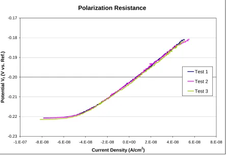
scan provides data that can be used to calculate a general corrosion rate for the sample. Figure 3.4 shows a set of three polarization resistance scans, performed one after the other with brief pauses to allow the potential to reach the open circuit level before re-testing.
Polarization Resistance
-0.23 -0.22 -0.21 -0.20 -0.19 -0.18 -0.17
-1.E-07 -8.E-08 -6.E-08 -4.E-08 -2.E-08 0.E+00 2.E-08 4.E-08 6.E-08 8.E-08 Current Density (A/cm2)
P
o
te
n
tia
l V
f
(V vs. Ref.) Test 1
Test 2
Test 3
Figure 3.4 Typical polarization resistance curves.
The slope of the polarization resistance curve has been shown to be inversely proportional to the corrosion rate (Jones, 1992). The relation was quantified using the software developed by GamryR, EchemAnalyst. EchemAnalyst uses the slope of the polarization resistance curve along with the density of the sample, the number of equivalents exchanged, the atomic weight, sample area, and Faraday’s constant to calculate a sample corrosion rate. This test is not destructive to the sample due to the small potential range that is scanned.
typically be modeled using an equivalent circuit of resistors and capacitors that pass current with the same amplitude and phase angle that the real cell does under a given excitation (Bard, 1980). A basic cell and circuit model that are used in this thesis are shown in Figure 3.5. This figure shows a solution resistance, double- layer capacitance, and a corrosion
Figure 3.5 EIS model of sample and equivalent circuit.
resistance for the solution, solution-sample interface, and sample respectively. While there is the possibility to calculate several useful properties of the solution and the sample, the chief objective of an impedance experiment is to discover the frequency dependencies of the solution resistance, Rs, and the double layer capacitance, Cdl (Bard, 1980).
EIS equivalent circuits can be modeled using mathematical descriptions of the electrical circuit. The time-dependent current response I(t) of an electrode surface to a sinusoidal alternating potential signal V(t) is expressed as an angular frequency (ω) dependent impedance Z(ω):
( )
( )
( )
( )
( )
(
)
sin sin o o V t Z I t V t V tI t I t ω ω ω θ = = = +
where θ is the angle between V(t) and I(t), and ω is the angular frequency as provided by the potentiostat perturbation (Jones, 1992). The impedance can be expressed in terms of real, Z’(ω), and imaginary, Z”(ω), components:
RE WE
( )
'( )
''( )
Z ω =Z ω +Z ω
(Jones, 1992). The data gathered from an EIS experiment provides a Bode plot of both the impedance and phase angle versus the frequency, and a Nyquist plot showing a semicircle of imaginary and real impedance with the frequency moving in a counterclockwise direction (Figure 3.6). This circuit is often an adequate representation of a simple corroding surface.
Figure 3.6 Equivalent circuit with a) Nyquist plot and b) Bode plot (Jones, 1992).
Notice the relationship between the solution resistance (RΩ) and the corrosion resistance (Rp)
which can be seen in both the Nyquist and Bode plots: at very high frequency, the imaginary component, Z’’, disappears leaving only the solution resistance. At low frequencies, the imaginary component disappears again, leaving the sum of the solution and corrosion resistance.
The GamryR software, EchemAnalyst, has the ability to perform analysis on EIS data, but it is best to know the equivalent circuit for the sample and solution being tested before performing the software analysis. Assumptions can sometimes be made and the model can be simplified. The analysis method used for this thesis is described in section 3.2.3. It was found that no single equivalent circuit model worked well for all samples tested. There was no consistency in any one model to allow useful reporting of the data.
dp cm w dt year ρAt
⎛ ⎞=
⎜ ⎟
⎝ ⎠
Where w is the weight loss in grams, ρ is the density in grams per cubic centimeter, A is the exposed area in square centimeters, and t is the time in years that the sample was exposed (Farmer et. al, 2000).
3.1 Apparatus, Materials, and Methods
Corrosion tests were performed at LLNL using the advanced corrosion testing facilities that have been used for Yucca Mountain corrosion studies for more than 10 years. The corrosion analyses at LLNL for Yucca Mountain follow strict quality assurance protocol to ensure defensible results and maintain consistency in all analysis, no matter who performs them or where they are performed. The corrosion studies performed on the samples for this experiment followed the same procedures as those used at LLNL.
Two different samples were tested for corrosion using two different methods: potentiostatic measurements on disk samples as described in the introduction and coating section of this thesis, and general corrosion of weight-loss samples in concentrated solutions.
3.1.1 Polarization Testing
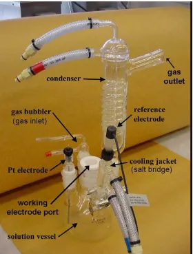
Potentiostatic corrosion tests were done using a Gamry Instruments Version 4.30 Potentiostat (PC14/300 model) with DC105 and EIS 300 capabilities. This potentiostat can control the electode potential within 1 mV of the preset value and has an anodic current range from 7.5 nA – 750 mA. The input impedance is >1012 ohms with an accuracy of ±0.3% of the voltage range or ±0.3% full-scale for the current. A three-electrode configuration with a platinum auxiliary three-electrode, silver/silver-chloride reference electrode (Accumet), and a test specimen/working electrode was the design used for testing. A solution volume of 950 ml with a nitrogen bubbler was used along with a condenser as the gas outlet. The solution was kept at temperature using a circulating oil bath with automatic controls for temperature stability and uniformity (PolyScience model 9112).
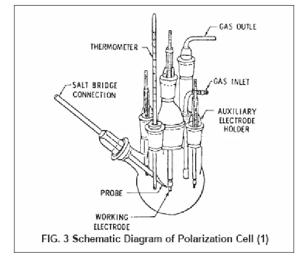
reference electrode, and the gas bubbler and condenser. A thermometer is often seen in designs such as this, but with the silicon bath, the solution temperature was checked just before and after testing and assumed to stay constant during the testing period. The Luggin probe-salt bridge maintained separation between the bulk solution and the reference electrode and also allowed for adjustment of the tip to be in close proximity of the test electrode. The glassware and material used for mounting and testing the sample can be seen in Figure 3.7 which closely matches the design as described in ASTM standard G5-94 on the Standard Reference Test Method for Making Potentiostatic and Potentiodynamic Anodic Polarization Measurements (Figure 3 in standard), Figure 3.8.
Figure 3.8 Schematic of polarization cell from ASTM standard G5.
Three basic experiments were carried out on the disk samples including cyclic polarization, linear polarization, and EIS tests. These tests were done following the ASTM standards for electrochemical measurements (G3-89, G5-94, G61-86, G106-89, etc.). The order of experiments was chosen to allow for as much data to be collected before the sample was destructively tested (cyclic polarization).
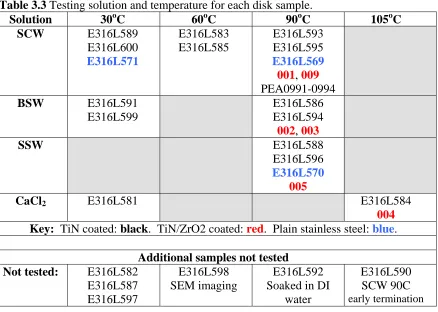
test. A solution pH measurement was taken before and after each test was completed. The testing configuration for solution and temperature level for each sample tested can be seen in Table 3.3.
Table 3.3 Testing solution and temperature for each disk sample.
Solution 30oC 60oC 90oC 105oC
SCW E316L589
E316L600 E316L571 E316L583 E316L585 E316L593 E316L595 E316L569
001, 009
PEA0991-0994 BSW E316L591
E316L599
E316L586 E316L594
002, 003
SSW E316L588
E316L596
E316L570
005
CaCl2 E316L581 E316L584
004
Key: TiN coated: black. TiN/ZrO2 coated: red. Plain stainless steel: blue. Additional samples not tested
Not tested: E316L582 E316L587 E316L597
E316L598 SEM imaging
E316L592 Soaked in DI
water
E316L590 SCW 90C early termination
The software used during experimentation and for analysis included Gamry Framework DC105 for corrosion testing, and Gamry EChem Analyst for data analysis. The Framework software provided a rapid non-destructive corrosion rate measurement and had a wide scan standard technique for most corrosion region studies as specified in ASTM standard G5.