Techniques to Improve the Usability of Software Signature Based Data Dependence Profilers for Feedback Driven Optimizations

(1)

ABSTRACT

SOLE, LAXMAN GHANASHAM. Techniques to Improve the Usability of Software Signature Based Data Dependence Profilers for Feedback Driven Optimizations. (Under the direction of Dr. James Tuck.)

The absence or unavailability of dependence information between individual memory

operations restricts the compiler’s ability to optimize code. Lack of information forces a

compiler to make conservative decisions and results in suboptimal transformations. At

a time when Moore’s Law is slowing down, speculative optimizations based on memory

dependence information can boost the performance by a significant margin. Data Depen-dence Profiling helps to tackle this problem by collecting the depenDepen-dence information at

run time. Collected information can be used as feedback to optimizations to achieve higher

performance. However, dependence profilers often incur large overheads, making them

impractical for widespread use.

Set-based profilers, studied in this dissertation, have the potential to significantly

re-duce dependence profiling cost, achieving its speed through approximate signature-based

dependence tracking. However, the approximate nature of signatures make them harder to

use. Signatures introduce false positives while tracking dependencies, making it difficult to

determine if a signature-based profile is accurate or not without a comparison to a more expensive analysis without signatures.

This dissertation addresses the usability of a signature-based profiler in two ways. First,

we propose a set of heuristics for estimating the accuracy of a signature profile, thereby

making it possible to know how trustworthy a profile is without running a more

expen-sive one for comparison. Second, we propose the idea of incremental profiling which is

performing profiling operations multiple times on a subset of queries to achieve the same

or better accuracy with a lower performance penalty. With the help additional heuristics

that we propose, incremental profiling has shown an overall reduction in overhead with an

improved accuracy.

Prior work observed a slowdown of around 14_×for an accuracy of 0.1 NAED. With our

new methods, we get the same accuracy with around an 11_×slowdown. Also, an accuracy

of 0.06 NAED can be achieved with a 12_×performance penalty. Also, various

optimiza-tions benefit from feedback using our profiles. LICM shows an improvement of 5.6% for

(2)

benchmarks on a 32-bit machine. When coupled with our dependence profiler, the SLP

vec-torizer pass in LLVM offers a performance improvement of up to 4.7% for the 183.equake

benchmark and an average performance improvement of 1.4% (geometric mean) was

(3)

(4)

Techniques to Improve the Usability of Software Signature Based Data Dependence Profilers for Feedback Driven Optimizations

by

Laxman Ghanasham Sole

A thesis submitted to the Graduate Faculty of North Carolina State University

in partial fulfillment of the requirements for the Degree of

Master of Science

Computer Engineering

Raleigh, North Carolina

2017

APPROVED BY:

Dr. Eric Rotenberg Dr. Huiyang Zhou

Dr. James Tuck

(5)

DEDICATION

(6)

BIOGRAPHY

The author has received his Bachelor of Technology in Electronics Engineering degree

from Vishwakarma Institute of Technology, Pune, India in 2013. He worked for Harman

International as an Embedded Software Engineer from 2013 to 2015.

The author joined NC State University in Fall 2015 to pursue Master of Science in

(7)

ACKNOWLEDGEMENTS

I would like to use this opportunity to thank all those who have helped me directly, or

indirectly to reach the point where I am today.

First of all, I would like to thank my advisor, Dr. James Tuck for all the support, the

guidance he provided me during the time of this research. He made ECE 566 as one of the

interesting classes for me. I would like to thank him for allowing me to do the independent

study with him which made me confident about research. Also, there were times when I was feeling low and I am glad that Dr. Tuck was there to boost my confidence. Thanks, Dr.

Tuck for always motivating me.

I would also like to thank my committee members: Dr. Rotenberg for making the

com-puter architecture a fun class and for spending most of his office hours explaining Trace

Processor and its consistency logic. And also, Dr. Zhou for helping me generate interest in

GPU architecture.

I would like to thank all my family members and my friends Mayur, Tejas, Sachin, Ravi,

Sunil, Swapnil, Ganesh, Anay, Sagar, Poonam, Yogesh, Amit, Sayali, Tushar who have always

wished the best for me. I would also like to thank my friends in Raleigh: my roommates Tanesh and Sushant, Prachi, Pooja, Himanshu, Heramb, Minal, Aish, Shardul, Prathamesh,

Karan, Puneet, Sarvagya, Ritesh, and Mahita. Thank you guys for being great friends and

support. Thanks, Apoorv and Kshitij for helping me take decisions and not getting annoyed

at me. Also special thanks to Aditya for the long discussions on almost all topics(!) and

Aishwarya(Your name is here!) for encouraging me to do this thesis.

This material is based upon work supported by the National Science Foundation under

(8)

LIST OF TABLES

Table 2.1 Signature Configurations[Par16] . . . 12

Table 3.1 Sample fpp Calculations . . . 24

Table 3.2 Predicted min and max values for the estimated perfect profile based on the heuristic . . . 25

Table 3.3 Average Percent Error of predicted Avg to NAED of Perfect Profiler . . 30

Table 4.1 SigProfiler Table . . . 36

Table 4.2 Perfect Profiler Table . . . 36

Table 5.1 Number of Load Instructions Hoisted . . . 62

(11)

LIST OF FIGURES

Figure 1.1 Example showing possible LICM optimization opportunity . . . 2

Figure 1.2 Query classification using static Alias Analysis . . . 3

Figure 2.1 DDP Tool Flow[Par16] . . . 7

Figure 2.2 Control Flow Graph with diverging control paths[Par16] . . . 9

Figure 2.3 Accuracy of profilers with varying signature size . . . 15

Figure 2.4 Performance overheads of profilers with varying signature size . . . . 17

Figure 3.1 Refid Classification . . . 22

Figure 3.2 Result for min-max accuracy for Signature of size 3k . . . 26

Figure 3.3 Sample data for Avg Calculations . . . 28

Figure 3.4 Result for min-max accuracy for Signature of size 3k with Avg value . 29 Figure 4.1 Percentage of Refid Coverage and percentage of refids with depen-dence in 1k Signature . . . 32

Figure 4.2 Performance comparison for Feedback Profiler and Perfect Profiler . 34 Figure 4.3 Performance comparison using Dependence Probability heuristic . 39 Figure 4.4 Accuracy comparison using Dependence Probability . . . 40

Figure 4.5 Percentage of refids considered for the second run . . . 41

Figure 4.6 Performance comparison using Function Execution Count . . . 43

Figure 4.7 Accuracy comparison using Function Execution Count . . . 44

Figure 4.8 Performance comparison of 2k and 8k signatures with 2k+Perfect and 8k+Perfect signatures . . . 47

Figure 4.9 Accuracy comparison of 2k and 8k signatures with 2k+Perfect and 8k+Perfect signatures . . . 48

Figure 4.10 Performance Comparison of 1k signature with ET and EET . . . 50

Figure 4.11 Percentage increase in code size for ET and EET wrt 1k signature profiler . . . 52

Figure 4.12 Performance Vs Accuracy results for different Incremental Profilers . 54 Figure 5.1 DDP Tool Flow[Par16] . . . 57

Figure 5.2 DDP Feedback Metadata in LLVM IR . . . 59

Figure 5.3 LICM Performance with DDP feedback(Only LICM ran after -O3 op-timizations) . . . 61

Figure 5.4 LICM Performance with DDP feedback(LICM ran after -O3 optimiza-tions with different Loop Size threshold) . . . 64

Figure 5.5 LICM Performance with DDP feedback(LICM ran after -O3 optimiza-tions with only modules containing hot funcoptimiza-tions optimized) . . . 65

(12)

Figure 5.7 Performance of SLP Optimization with DDP Feedback information . 69 Figure 5.8 Profiler Accuracy Vs useful Information . . . 70 Figure 5.9 LICM Performance using different Profiler configurations of varying

accuracy . . . 72 Figure 5.10 Standalone SLP performance for 183.Equake benchmark with varying

(13)

CHAPTER

1 INTRODUCTION

Along with enhancement in hardware technology, software has also played a major role in

keeping Moore’s Law going. With increasing complexities of hardware, it is the responsibility

of software to use hardware resources in optimal ways to achieve high-performance and

efficiency. Most of the time software or compiler optimizations make very conservative

decisions due to a lack of information that is required for a particular optimization. One

such case is with memory dependence information. Prior works have demonstrated the

importance of incorporating runtime information in speculative optimizations for the

(14)

1.1 Data Dependence Problem

When data produced by one instruction are required for the execution of another

instruc-tion, it is called a data dependence. This may also be called a def-use or producer-consumer

relationship. For non-memory instructions and some memory instructions also, we can

easily determine the data dependence relationship just by static analysis of the code. If the

dependence is through memory operations, then static analysis may fail to determine the

absence of a dependence. This is a very common scenario in programs.

In many optimizations, knowing this information helps the compiler optimize the

program in a much better way. Let’s consider the same example as discussed in[Par16]. This example demonstrates the need for dependence information in Loop Invariant Code Motion (LICM). Figure 1.1 show the representative code.

Figure 1.1Example showing possible LICM optimization opportunity

In this example, if the compiler knew in advance that the variables a and b point to

different locations in memory, then it can simply move the computation of ‘temp’

vari-able outside the loop as both of its operands are loop invariant. This would save a lot of

redundant computation. Compilers mostly rely on Static Alias Analysis for this information,

but if alias analysis is unable to prove the absence of a dependence, then it reports the dependence as MayAlias, which is ambiguous in nature. Figure 1.2 show the percentage of

MustAlias, PartialAlias, NoAlias, and MayAlias reported by Alias analysis. Queries are from

(15)

it is showing 30% queries as MayAlias, we are querying Alias Analysis using all possible

load-store instruction pairs, and there are many obvious NoAlias queries. Most of the time

this is not the case for the optimizations, and critical queries are often ambiguous in nature,

adding constraints on the optimization.

Figure 1.2Query classification using static Alias Analysis

Data Dependence Profilers (DDPs) collect dependence information at run time, and

this profiled information can be fed back to compiler optimization as a feedback. The next

(16)

1.2 Background

As mentioned in[Par16], we can make the four categories of the different approaches[Bru00; Che04; Kim10; VT12; Fax08; Zha09; Wu08; YL12b]taken for data dependence profiling.

1. Shadow Memory based Profiling:

[Che04]describes this approach in detail and it has been used in other prior work

[SM98; Liu06; Udu11]. This approach uses a single structure which is representative of the entire memory. Also, instead of instructions keeping track of all the memory

locations it has accessed, in this approach the memory locations keep track of some

n latest instructions which have accessed it. New incoming instructions replace the

information of the oldest instruction. In the end, we can have dependence

infor-mation in the form of a chain of dependence. Dependence inforinfor-mation between

load-store, store-load, store-store, or load-load can be recorded separately for later

usage. Shadow memory can be implemented using virtually unlimited hash-tables

(actually limited by the main memory size) to keep track of all the operations which have accessed a particular location. There can be smaller hash-tables which maintain

the fixed number of latest operations which have accessed a particular location in

memory. This involves high operational overheads per memory operation in terms of

accessing and updating the hash-tables. Also, hash collisions are the main reason for

the inaccuracy in these profilers.

2. Pattern Driven Profiling:

Instead of tracking dependence between all possible memory instructions, Pattern

Driven Profiling approach[Kim10; Bru00]focuses on particular memory operations like those in hot path of the code, and it looks for the particular access patterns like

stride access of dependence between different loop iterations. This technique also

focuses on getting a high-resolution view of the dependence i.e. it tries to determine

iteration-wise dependencies to parallelize the iterations if there isn’t a loop-carried

dependence.[Kim10]suggests a use of parallel computing to reduce the profiling overheads only up to 10-20x slowdown. Though the technique provides dependence

(17)

its usage in a larger scale.

3. Offloading Profiling for Efficiency:

[Kim10; YL12a; YL12b]suggests techniques like slicing, novel parallel algorithms to use parallel computing resources in Data Dependence Profiling. Parallelization reduces

the performance penalty to a great extent. Also, in general, due to very localized nature

of memory access pattern, load balancing across different threads is a challenging

task.

4. Set-based Profiling:

In this approach, Vanka and Tuck[VT12]uses a separate data structure(set/signature) to track dependences between a pair of instructions. This helps in isolating the two

unrelated references to avoid the degradation of accuracy due to their interference.

The intuition behind using a separate structure for each instruction is that individual

memory operations will not access too many different locations. This set/signature based approach has proven relatively lightweight and shown the effectiveness in profiling with respect to accuracy and performance overheads.

1.3 Contribution

This dissertation extends the set-based profiling approach and proposes techniques to

improve its usability for feedback-driven optimizations. The first technique is a heuristic

to predict the accuracy of the signature based profilers. This technique eliminates the

requirement of a costlier Perfect Profiler for accuracy calculation. With the second technique of incremental profiling, we can reduce the performance overheads with achieving high

accuracy. It also evaluates the performance of LICM and SLP Vectorizer using the DDP

feedback information.

The subsequent chapters talk about the DDP tool flow, accuracy prediction heuristic,

proposed incremental profiling technique and evaluates the optimizations using DDP

(18)

CHAPTER

2 SOFTWARE SIGNATURE BASED DDP

Chapter 1 discusses the dependence problem and various approaches of data dependence

profiling. This chapter is going to talk about the overall flow and decision choices for the

Software Signature based Data Dependence Profilers (DDP) proposed by Vanka and Tuck

[VT12].[Par16]also discusses the similar things about the DDP tool. In this code instru-mentation based DDP, the dependence between a load and a store instruction is tracked by

assigning one set or signature (discussed in detail later in Section 2.1.3) per load-store pair

or multiple pairs and by performing address insertion into the signature and checking for

membership into it. These signatures can be considered as a compact view of the entire address space for the load and store in that particular pair. It is a compact view because we

store only addresses accessed by the store instructions and not all possible addresses. This

per-pair signature approach isolates dependence information of individual queries. Also,

the number of addresses accessed by any particular store are relatively fewer, which leads

to a smaller signature size and faster access to it, reducing the profiling overheads. Section

(19)

2.1 DDP Tool Flow

(20)

Figure 2.1 shows the overall work-flow of Software Signature based DDP(henceforth

only referred as ‘DDP’). In this chapter, we will only discuss the profiling part of the DDP

Tool. Feedback Directed Optimization part is discussed in Chapter 5. As mentioned in

[Par16], code instrumentation for DDP can be performed at 3 stages:

1. Binary/ISA instructions

2. Intermediate Representation

3. High-Level Language

This profiler instruments the code at LLVM intermediate representation (IR)[Llv] level. This is because most of the compiler optimizations which are going to use the profiled

information also operate on the LLVM IR. So it will be convenient if we have the information

at the IR level. Also at C/C++level, there is a lot of unnecessary data for instrumentation because most of the high-level code gets optimized after certain compiler passes. The binary

level code does not have high level information required by the subsequent IR optimizations. Also, register allocator adds extra loads/stores in the binary. These loads/stores due to fills/spills also get considered for the instrumentation which are completely unnecessary. The whole infrastructure has been developed as an LLVM tool which operates on LLVM

IR. To minimize the overheads of extra instrumentation, we have used -O3 optimized IR as

input to the tool which ensures a fewer number of loads and stores. The implication of this

is discussed in Chapter 5.

Following subsections discuss the important stages of the profiler architecture.

2.1.1 Query Generation

DDP collects the dependence information at the granularity of pair of any two memory

operations whose dependence information we want to collect. However, this profiler only

collects dependence information of a pair of a Load and a Store instruction. We refer to this pair as ‘Query’ and assign a unique reference identifier to it known as ‘RefID’ or ‘refid’.

Refids help us to keep track of all unique load-store pairs across multiple modules and

(21)

costly operation(Section 2.3 talks about it). To minimize the performance penalty, we can

intelligently omit certain queries from the instrumentation.

We used following two methods for the same:

2.1.1.1 Diverging Control Paths

Figure 2.2Control Flow Graph with diverging control paths[Par16]

Sometimes it is possible to determine an absence of dependence between a Load and a

Store, by just observing their positions in a Control Flow Graph (CFG). One such case is

when a Load and a Store are in the mutually exclusive path. In that case, we can simply

discard the query and improve a performance. In Figure 2.2, Load A and Store B are in a

mutually exclusive path, so they will not have any dependence. However, for Load C and

(22)

if they cannot show dependence in the same iteration, there is a possibility that they are

accessing the same memory across multiple iterations. Therefore, we have to consider such

queries for instrumentation.

2.1.1.2 Static Alias Analysis

In general, the compiler uses Static Alias Analysis(AA) to determine the dependence

be-tween two memory instructions. AA gives the results in terms of ‘MustAlias’, ‘NoAlias’ and

‘MayAlias’. If AA returns MustAlias/PartialAlias or NoAlias, this means that the compiler is statically able to determine that there is either dependence or no dependence respectively.

In this case, we do not consider such queries for instrumentation and only consider the

ambiguous MayAlias queries. This saves some unnecessary instrumentation.

2.1.2 Set Assignment

Once we have all the queries, we assign set/signature to each of the queries. Multiple queries sharing the same store, get the same set/signature. We can also combine multiple stores intelligently and assign them a single signature. This will reduce the number of signatures and cost of initialization and deletions associated with each signature. However, if multiple

stores share the same signature, then we cannot tell the exact dependence information

relation between a load and one of the stores which share the signature. This adds the

ambiguity and reduces the accuracy. In this dissertation, we have considered a separate

signature for each Store instruction in a query.

2.1.3 Instrumentation

At this stage, we have all the queries and sets assigned to them. The instrumentation involves

assigning a particular type of signature to each set, initialization of that signature, assigning

and initialization of local and global variables, and finally freeing the signature. All these

factors keep track of the dependence and other information related to the query. There

are two major operations involved in checking the dependence. First, at store instruction in the query, we insert the address accessed by that store into the signature and at each

(23)

membership check in that signature. Based on the membership results, local and global

variables, tracking the dependence information can be updated. It is possible that multiple

loads are checking dependence against a particular store simultaneously and vice-versa. In

case of one store and many loads, there will be only one signature corresponding to that

store and each load has to perform membership-check against that particular signature. In

case of multiple stores against a single load, the load has to perform the membership-check in all the signatures corresponding to each store.

2.1.3.1 Bloom Filter based Set Implementation

The number of sets/signatures are proportional to the number of queries in a program. So we can expect a large number of signatures to be added after the instrumentation. So to

keep the overall cost of profiling low, all the operation related to each set e.g. initialization,

insertion, membership-check, and deletion have to be fast. Vanka & Tuck[VT12] have proposed "software signatures" based on Bloom Filter[Blo70]to achieve this. Bloom filters are simple bitmaps or the binary arrays which can be indexed using hash functions. Due to

use of hash function for the indexing, bloom filters have probabilistic nature. One of the

important properties of bloom filters is that a bloom filter never gives the false negatives

i.e. even if a member is not present in the bloom filter, it may say it is a member (False

Positive) but if the member is present in the bloom filter, it will never say it is absent (False

Negative). Because of this nature, the dependence information we get can be conservative

in nature, but it will not affect the correctness of the application that has been optimized

using this profiled information.[Par16]discusses the working of bloom filter in detail and also introduces the banked bloom filters or banked signatures to improve the accuracy. In banked bloom filters, each bank has its hash function and uses different ranges of memory

address bits for the hashing. Table 2.1 show the configurations of signatures used in this

(24)

Table 2.1Signature Configurations[Par16]

Signature Banks Bank Size Index bits per bank Utilized bits of hash

1K 2 512 9 18

2K 2 1024 10 20

3K 3 1024 10 30

8K 2 4096 12 24

2.2 Accuracy

Signature based profilers are probabilistic in nature because of the use of bloom filters. Due to this, the profiled information cannot be correct all the time. Though we do not have

false negative information (thanks to bloom filters), there is some false positive data. It is

important to know the degree of accuracy/correctness of the information we have for a particular program. So we calculate the accuracy of the profiler by comparing it with the

results of Perfect Profiler. Next subsection explains the Perfect Profiler.

2.2.1 Perfect Profiler

Perfect profiler follows the same flow of instrumentation as signature based profiler.

How-ever, it differs from signature based profiler in the following aspects:

(a) Memory usage: Signature based profilers use statically assigned fixed amount of

memory for each set. Perfect profiler uses STL’s std::set[ISO14]data structure for signature implementation which assigns memory dynamically, as and when the new

element is inserted i.e. it is assumed that it can use an infinite amount of memory if

required.

(b) In bloom filter based signatures, only a few bits of the address are used to represent the

address and stored in the limited size structure. Perfect profiler stores entire addresses.

Therefore, it never suffers from the aliasing problems due to hash collisions or limited

(25)

Dynamic memory allocation and traversing such data structures is a very slow operation,

and hence the perfect profiler has a very high overhead. Also, some benchmarks fail during

execution of perfect profiler because of its large memory requirements.

2.2.2 Normalized Average Euclidean Distance

We have used Normalized Average Euclidean Distance(NAED)[SS06]as our accuracy metric. NAED for any profiler is calculated against the perfect profiler using following formula:

N AE D =

v u u u t n X i=0

(pi−si)2

n (2.1)

Herepiandsiare the dependence probabilities of a particular query ‘i’ in the perfect and signature based profiler respectively. Dependence probability is a fraction representing the

number of times a certain query showed dependence out of the total number of times a

function was executed. Section 4.3 and 4.4.1 give a clearer picture of database entries and

the Dependence Probability.

If the two profiles have the same dependence vectors i.e. all the queries show the exact

same dependence using two different signatures then they have the same accuracy. From

the Equation 2.1, it is clear that NAED will always have the value between 0 and 1. Value 0

implies that both the profilers have the exact same dependence vector while value 1 implies

they are totally on the opposite sides of the spectrum. Suppose if out of the 100 queries all of them show a dependence off by 30% then NAED would be 0.3, on the other hand, if only 30

of them are off by 100% then NAED will be 0.5477. This shows that NAED value is affected

by both the number of mismatching queries and the margin by which they mismatch.

One criticism about this metric is that it considers all the queries in the same way. This

is mainly because we consider the probability value to calculate the distance between two

vectors and by the nature of probability we have the normalized values. We loose the

infor-mation of individual queries in the process of normalization. So if less frequently executing

queries show false dependence only for some of the times when there is no dependence,

its Dependence Probability is higher than the one which also shows dependence for the

(26)

queries contribute by a large value towards NAED. We have used this fact to our advantage,

and Chapter 4 discusses this in detail. Using this metric, we can compare different profilers

even if they have different configurations. The goal is to keep the NAED value close to 0

with respect to the Perfect Profiler. Section 4.3 shows the example of accuracy calculation

and Section 5.6 discusses the significance of this metric in detail.

(27)

(28)

2.3 Profiling Cost

As we are adding extra code for each query, it adds extra overheads to the program. This

cost can be divided into following factors:

(a) Direct Overheads: This involves the cost of signature initialization, address insertion,

membership check, memory freeing cost for each query. Multiple queries with the

same store instruction share these costs. As signature size increases, the initialization

cost increases as well. Also, if we use multi-bank signatures, it increases the cost of

insertion and membership-check, as the number of hash functions increases by the

same factor. Apart from the signatures, we need some local and global variables to keep track of dependence. Their initialization also adds extra cost.

(b) Indirect Overheads: In these types of overheads we consider the effect of code

bloat-ing. Due to instrumentation, the code size increases drastically. Increased code size

increases the pressure on I-Cache. Also, signatures are a part of the working set of the

program, and they can pollute the data cache which can harm the performance.

In-creased local/global variables increase register pressure which adds to the overheads.

2.4 Experimental Setup

We used both integer and floating-point benchmarks from SPEC2000 and SPEC2006 for

the evaluation. Benchmarks’ binaries of different configurations are evaluated on High

Performance Computing(HPC) systems. Each HPC node comprises of Intel® Xeon®

Pro-cessor E5520 which runs 8 threads on its 4 cores and has 8MB cache. It has 23GB main

memory with 32GB swap space and runs RHEL7 OS. Binaries are compiled for 32-bit X86

architecture. Also, all the 8 threads are dedicated to the same program in order to avoid

any slowdown due to other running workloads. We have used LLVM version 3.6.2 for all

evaluations. Performance is measured as speedup or slowdown against the -O3 optimized code.

Figure 2.4 shows the slowdown caused by different profilers w.r.t. -O3 optimized

(29)

(30)

2.5 Previous Work

From figure 2.3 and 2.4, we can see that Perfect profiler has very high overheads with 100%

accuracy while other profilers are relatively fast but are inaccurate. This section talks about

the previous efforts to achieve high accuracy with low overheads in software signature

based DDP. Detailed explanation and reasoning behind these techniques are discussed in

[Par16].

2.5.1 Heuristic based pruning of refids

As discussed in Section 2.1.1, we can discard some of the queries on the basis that these will

always show either dependence or no dependence. We had discussed queries in divergent

control flow and MayAlias queries. Here are some more heuristics using which we can

statically decide the dependence information of certain queries and save performance by not instrumenting them:

1. Constant Data Space: As it is illegal to modify the constant data space, a load

instruc-tion loading from constant memory will never conflict with a store instrucinstruc-tion.

2. Structure Type Mismatch: This heuristic is based on the assumption that two different

structures should not conflict with each other as they will have different memory

footprints. However, this heuristic fails in the case of nested structures and in the

case where a structure is cast from one type to another.

3. Structure Index Mismatch: Different elements of the same structure should never conflict with each other.

4. Local Variables vs. Unknown Aggregates: Local variables should not conflict with

aggregates because we can trace back their allocation on the stack.

5. Local Structures vs. Function Arguments: Variables declared inside the function

cannot conflict with the function arguments even if all of them are on the same stack.

6. Local Variables with No Pointers: Most of the time local variables are not manipulated

(31)

So they can never have a conflict with other addresses.

Some of these heuristics give false negative results. We cannot use these heuristics if we are

going to use profiled information as a feedback for the compiler optimizations because it

will affect the correctness of the optimization.

2.5.2 Range Set

Range set leverages the fact that most of the memory accesses have spatial locality. So

instead of tracking all the addresses accessed by the store instruction, range sets track the range of these addresses. Membership-check is positive for the addresses which fall into

this range and negative for the addresses outside the range. This technique has very lower

overheads as we just have to monitor two ranges. This technique works nice with very small

range i.e. densely packed memory accesses but is poor with sparse access patterns. Range

sets cannot distinguish if any particular address which falls into the range has actually

accessed memory or not. This adds inaccuracy to this technique.

2.5.3 Hybrid Set

This combines the Range Set based technique with bloom filter signature and tries to get

the best of both worlds. In hybrid set implementation, during the insertion operation, an

address gets added to bloom filter and it modifies the range as well. For membership check,

on the one hand, if the address is outside the range then it can be directly considered as a non-member (this is an inexpensive operation), on the other hand, if the address falls in

the Range then the bloom filter can be used to decide the membership.

The next chapter will discuss the first proposed technique to calculate/predict the accuracy of signature based profilers (against perfect profiler which gives 100% accuracy)

without actually needing the perfect profiler’s information. Subsequent chapters discuss

the second proposed technique of incremental profiling to achieve the balanced profiler

(32)

CHAPTER

3 ACCURACY PREDICTION

As mentioned in Chapter 2, the signature based Data Dependence Profilers are probabilistic.

Probabilistic nature of these profilers makes it tough to know how accurate they are in

general. The accuracy of these profilers has been calculated in terms of NAED, and we

need perfect profilers for such accuracy calculations. Figure 2.4 shows the performance

overheads of the perfect profilers which can go from 10x to few 100x the run time of the

original program. Also, the assumption about perfect profiler is that it can use an infinite

amount of memory. Some programs when instrumented for perfect profiling uses a huge

amount of memory and hence failed to execute due to lack of memory. To run such profilers every time on the comparatively larger set of data is a very costly operation.

So this chapter describes the heuristic with which we can determine the accuracy of

these DDPs without an actual comparison to the perfect profiler. Using this heuristic based

accuracy, we should be able to identify whether a chosen signature configuration is working

properly or not on a given set of data. Also, prediction of accuracy is necessary since practical

(33)

3.1 Approach

As described in Section 2.1.3, Software Signatures in DDP are implemented using Bloom

filters. Characteristic of a bloom filter is that it can give false positive results, but it never

gives a false negative result. That means if there is no dependence for a particular refid then

it might say there is a dependence (false positive), but if there is dependence, then it will

never say there is no dependence. Because of this nature of Bloom filters, the results we

get are conservative in nature, but they don’t affect the correctness of code which has been

optimized using these results.

To study the behavior, refids can be classified into four sections as follow ( Here ‘Count’

indicates the number of times a dependence edge is observed) :

(a) Count matching with Perfect and Perfect Count is zero (matching zero): Both perfect

and signature-based profiler measure a 0 chance of dependence. No false positives

occurred, and, importantly, we know the profiled result was accurate for this refid.

(b) Count matching with Perfect and Perfect Count is non-zero (matching non-zero):

Both profilers produce the same non-zero probability. No false positives occurred,

but we cannot know this without running a perfect profile.

(c) Count not matching with Perfect and Perfect Count is zero (non-matching zero): Dependencies are detected by the signature-based profiler, but, in fact, none were

detected by the perfect profiler. In this case, only false positives are measured.

Unfor-tunately, we cannot distinguish this case from matching non-zero without additional

information.

(d) Count not matching with Perfect and Perfect Count is non-zero (matching

non-zero): The two profilers disagree on the dependence probability, but neither is zero.

The difference is caused by false positives, so the signature-based probability must

(34)

Figure 3.1Refid Classification

From Figure 3.1 we can see that higher the % of ‘matching zeros’ means that particular

signature size gives more accurate results and lower value in terms of NAED. Also

‘non-matching zero’ and ‘non-‘non-matching non-zero’ are false positives, resulted from the over

population of signatures. Also, whatever NAED value we get, it is because of these false positive data. So to guess/predict the overall accuracy, we need to guess/predict the perfect profiler counterparts of these non-matching values. It is tough to distinguish between

two non-zero values and guessing which one’s perfect counterpart will be zero and which

one’s is non-zero. We use this observation as part of the basis for our accuracy prediction

(35)

3.2 Heuristic

Hash functions used to map the number of keys into bloom filter are supposed to be

perfectly random. The two reasons why bloom filters give false positive are

1. Over population of the signature

2. Non-random hash function

Assuming k hash functions used to hash n number of keys into m size bloom filter, after

hashing all the keys of set S into bloom filter, the probability that a particular bit is still 0 is,

p≈e−k n/m (3.1)

So for an address which is not present in signature but still passing the membership check

(i.e. for a non-member), it may be found to be a member with false positive probability

[BM04],

f p p≈(1₋p)k (3.2)

In DDP context, m is the size of the signature, n are the number of addresses a particular

store has accessed, and k are the number of hash functions used. DDP uses a single hash

function, so the value of k is 1, and it is assumed that our hash function is a random hash

function. For the number of keys, we assume that the number of set bits in a signature (population) are the number of hashed keys in it. So using these basic assumptions, we

calculated the approximate False Positive Probability (fpp) for each refid, as each refid has

a bloom filter associated with it.

In the previous data, we observe that most non-zero refids are non-matching zeros

dominated by a high false positive rate. We expect these refids to have a high likelihood of

false positive, and based on analysis, we determined this to be true. This leads us to the

following heuristic, empirically derived based on our data: if the fpp>51%, we predict that the refid is a non-matching zero. Note, an fpp of 51% implies that 75% of all bits are filled in

the signature. Hence, this is a conservative threshold, and we are likely to only classify the most egregiously overfilled signatures with this rule. Hence, this will only capture some of

(36)

Table 3.1Sample fpp Calculations

Sig. Size(m) Sig. Popultion(n) fpp

1024 100 0.09304

1024 250 0.21662

1024 500 0.38632

1024 750 0.51926

1024 1024 0.63212

Table 3.1 gives the few sample calculations of fpp for signature of size 1024 size.

3.3 Estimating the Perfect Profile (Min and Max values)

To estimate the accuracy, we predict the likely values produced by a perfect profile and

then calculate distance with respect to that prediction. Hence, we must predict the impact

on NAED of each refid separately and then compute the overall NAED.

To bound the error of our prediction, we predict both a min and max value for NAED.

The min would tell us the best interpretation of accuracy possible while max tells us the

worst interpretation possible based on our profiled result and heuristic. In the absence of

any information, it’s possible that all refids were measured accurately. This is the best case

scenario and reflects the min value. In the worst case, each refid was incorrect.

The worst possible scenario is that it predicts a dependence when there was not one. This corresponds to the max value. This may be unintuitive at first, but consider that the

signature profiler overestimates in the worst case. Its value can’t be smaller than the perfect

profile; it can only be larger. So, to maximize that error; we must assume the perfect profile

would have indicated no dependence.

For refids that exceed the fpp threshold of 51%, we assume these refids are actually

non-matching zeroes. As a result, in both our min and max estimation, we assume them to

be 0 and therefore must match with perfect. This is reasonable given the overly conservative

(37)

For all other refids with a non-zero dependence probability, they could fall into either

the non-matching zero, matching non-zero or non-matching non-zero category. In all cases,

we assume that the best case (min) is that the measurement matches perfect, and in the

worst case (max) the measurement should have the largest possible distance. This implies

that the maximum inaccuracy is achieved when the perfect profiler reports no dependence

and the signature profiler reports a large probability. These decisions are summarized in Table 3.2. Here,P_refid is the dependence probability for a single refid.

Table 3.2Predicted min and max values for the estimated perfect profile based on the heuristic

Refid Min Max

fpp>51% 0 0

fpp<51% P_refid 0

matching zero 0 0

We plot the results of the min and max distance prediction in Figure 3.2 along with

the real distance. This method is able to bound the actual value within the min and max

predictions. In general, if a benchmark has a small min and max value, it suggests that the

particular signature behavior is good.

For many benchmarks, the min value is predicted to be 0 but not in all cases. For example,

our prediction produces a very tight bound for 473.astar and 254.gap. The max value varies

significantly, and this is because max often measures the distance from the origin, giving a very conservative result. For example, the max prediction for 179.art is much worse than

(38)

(39)

3.4 More Precise Value

3.4.1 Need of another Value

If we see min and max range in Figure 3.2 for different signatures, the difference between

min and max for benchmarks like 179.art, 188.ammp, 256.bzip2 is more than 0.2 NAED.

For benchmark 188.ammp min value is zero and max is around 0.7 NAED. Even though

we know that actual value must be within these bounds, this is a much wider range. To

reduce this range further and narrow down the real value (closer to min value or max value),

we need another third value. We used the following heuristic to calculate this value. We decided to call this third value as avg even though it is not the exact average of min and

max.

3.4.2 Avg Calculation

We calculate an average predicted distance for all refids by decrementing the fpp threshold

over a range. This gives us an idea of how the min value changes with different thresholds.

We assumed the perfect counterpart as zero if fpp is above the threshold and same as our

value if it is below the threshold.

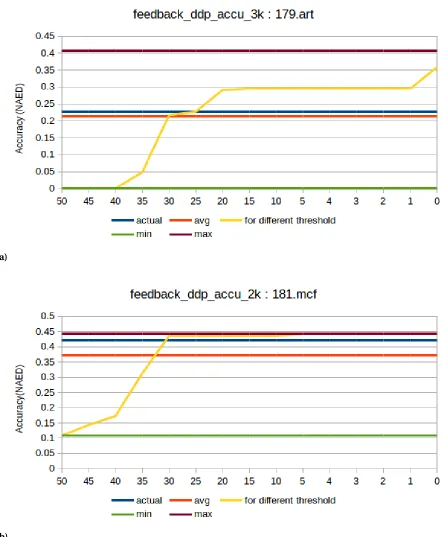
In Figure 3.3, we vary the fpp threshold (x-axis) and plot the resulting NAED according

to the min heuristic (the yellow line). The actual line is the true distance to perfect. The min

and max are calculated as before. The avg line is the average for the yellow line across all

thresholds for the distance. We can observe that the NAED value remains constant below a particular threshold and the benchmarks for which NAED is calculated w.r.t. the perfect

profiler, NAED lies around that value. Interestingly, this methodology works well for all the

applications. Table 3.3 shows the average percent error of our predicted NAED compared

to the true accuracy for several different signature configurations. We also show the average

(40)

(a)

(b)

(41)

(42)

We are now able to predict the accuracy in terms of NAED value if we have signature size,

number of hash functions used and population counts for a particular signature. Though

this number is not exactly matching with the NAED we get when we calculate it w.r.t. Perfect

Profiler, it has a reasonably small error on these workloads. Table 3.3 shows the percentage

error in prediction. With this, we can determine how good a particular signature is for the

particular benchmark. We can further use this information to develop a more accurate DDP with very less execution overhead.

Table 3.3Average Percent Error of predicted Avg to NAED of Perfect Profiler

Profiler Config. Avg Value Mid Value

(Predicted Value) (AM of Min-Max Values)

1K-Signature 5.5% 17.1%

(43)

CHAPTER

4 INCREMENTAL PROFILING

A DDP is useful if it has the maximum accuracy (i.e. 0 NAED) and a minimum performance

cost. Chapter 2 discusses the previous efforts such as different signature sizes(e.g. 1k, 2k,

3k, 8k), Range Sets, Hybrid Sets, selecting few refids for instrumentation based on a static

heuristic, to achieve the higher profiling accuracy with lesser performance overheads.

Though these techniques are very effective, there is also scope for improvement and goal is

always to achieve maximum accuracy with minimum overhead. This chapter discusses the

new approach of incremental profiling and its evaluation. Incremental profiling is simply

put doing profiling multiple times (currently set to two times) with successor run being incremental over its predecessor to achieve more balanced profiler in terms of accuracy

(44)

Figure 4.1Percentage of Refid Coverage and percentage of refids with dependence in 1k Signa-ture

4.1 Motivation

Figure 4.1 shows the percentage of total refids, which shows dependency in the signature

of 1k. There are only 7.5% (geometric mean) of these refids. If we consider the classification

in Section 3.1, these are all non-zero refids and out of these the only refids which belong to

type (c) and type (d) in Section 3.1 contribute to the inaccuracy or non-zero NAED value.

As discussed in Chapter 3, some of these refids are actually dependent, and some of

them show dependence due to the false positive nature of the signatures. So if we only

instrument these 7.5% refids with the perfect signature, run the profiler for the second time

and combine the data collected by both these runs, the effective profiler that we get by this

(45)

4.2 Main Idea

The key idea of incremental profiling is to run faster but a lesser accuracy profiler first;

use the data collected by this profiler as feedback and then run profiler one more time

with only a few refids instrumented either using a bigger signature or perfect signature.

Software Signature Based DDP uses SQLite Database[Sql]to store the profiling information collected by the profiler. The convenience of storing and querying of information allows us

to run profiler multiple time and update selective data from the older profiler without any

significant changes to the DDP tool.

Also, it is assumed that second run will take very less execution time as compared to

the first run. This is because we are instrumenting very few refids (only around 7.5%) for the second run. Less instrumentation leads to small code size, less overall local/global variables, fewer insertion/membership-check operations, and fewer signatures too. All these factors have a significant impact on the performance. Thus, we also hypothesize that

the combined execution cost of both of these runs will be significantly less than that of

the perfect profiler. This will achieve our goal of having 0 NAED with lower performance

overheads.

With this technique, there is some redundancy involved. With reference to Section 3.1,

we consider refids which fall into type (b) for the instrumentation in the second run. Even

if these refids are exactly matching with the perfect, we don’t know that in advance, and we have to pay the cost of initialization of local/global variables, signature initialization, and insertion/membership-check operations for these refids. Also, we have to execute the part of the code which does not contain any refids. One optimistic assumption here is that even

with these redundancies, the combined cost will be less than the perfect profiler.

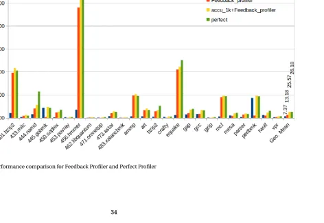
Figure 4.2 compares the slowdown for 1k Signature Profiler, feedback based second run,

(46)

(47)

From the Figure 4.2, it is clear that, even if we have gained some performance with

this technique, this is not a significant improvement. For benchmarks 401.bzip2, 433.milc,

473.astar, 188.ammp, 179.art, and 181.mcf, the combined overheads are more than the

perfect profiler. One of the important reason for this is, for all these benchmarks the

per-centage of refids which show the dependence out of the total covered refids is very large

(mostly greater than 40%. Refer Figure4.1). One of the reasons for most of these refids to show dependence with faster 1k-Signature is overly populated signatures. This also means

that most of these refids execute too often and accesses the wide range of memory causing

multiple keys to store in the limited size signature. This kind of behavior can be observed

in the case of a Store inside a big loop. For benchmarks 445.gobmk, 253.perlbmk, the

com-bined execution time is mostly dominated by the execution time taken by 1k-Signature

profiler where 1k itself takes time equivalent to perfect for the profiling.

Also, 186.crafty and 164.gzip benchmarks show perfect results with 0 NAED value. These

and other benchmarks with promising results with the faster profiler don’t need a second

run. With this technique, we can selectively choose to spend our computational resources in order to achieve higher accuracy. Correlation of accuracy with the actual useful information

(48)

4.3 Accuracy Calculation

Let’s consider an example to calculate the accuracy of signature profiler in terms of NAED.

We always calculate accuracy with respect to the perfect profiler. Assume we have a small

program with only 4 refids and we have its profiled information in the form of Table 4.1

and Table 4.2.

Table 4.1SigProfiler Table

Refid Count Totcnt

1 0 1

2 1 1

3 100 500

4 5 5

Table 4.2Perfect Profiler Table

Refid Count Totcnt

1 0 1

2 0 1

3 10 500

(49)

Accuracy of SigProfiler in this example will become:

N AE D =

v u u u t n X

i=0

(pi−si)2

n (4.1) = v u u t( 0 1− 0 1)

2_{+ (}0 1−

1 1)

2_{+ (} 10 500−

100 500)

2_{+ (}5 5−

5 5)

2

4 (4.2)

= 0.50803 (4.3)

From this example, we can see that not all refids contribute equally to the final accuracy value. Here 0.5 value comes from inaccuracy in refid number 2 and remaining 0.00803

comes from the inaccuracy in refid number 3. One more important thing to notice from

this example is, for any particular refid, if there exists a non-zero distance and a high Totcnt

(Function execution count), then that refid contributes by a very small fraction towards

the accuracy. Following Section 4.4 describes some of the heuristics we come up with to

(50)

4.4 Feedback based heuristics

From the previous section, it is clear that if we have to achieve 100% accuracy, we need to

pay certain performance cost. However, this relation between accuracy and performance

cost is not a linear one. If we intelligently select only a few refids which matter the most for

accuracy and have less performance overheads, then we can get the most balanced profiler.

This section talks about some heuristics which help us in selecting the right refids which

satisfy our requirements.

4.4.1 Dependence Probability

Dependence probability is the ratio of observed dependence to the number of time the

particular function is executed. Dependence counter is captured as ‘Count’ and function

execution count as ‘Totcnt’ in the database. SoCount/Totcntgives the dependence proba-bility.

So the observation is, if this probability value is higher and the corresponding probability

in perfect profiler is zero or negligible, then that particular refid is contributing to final

inaccuracy (NAED value) by the large factor. So to choose such refids, we assume several

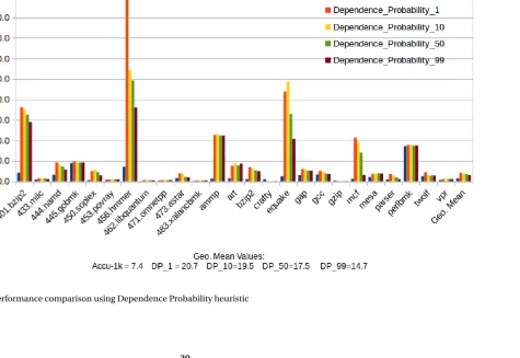
thresholds of the dependence probability for the experiments. Figure 4.3 and Figure 4.4

show the performance and the accuracy results with different threshold values.

Note that the slowdowns in Figure 4.3 for different DP_Profilers includes the cost of the

first fast run (which is 1k-signature profiler in this case). This is true for all the incremental

(51)

(52)

(53)

Figure 4.5Percentage of refids considered for the second run

Figure 4.5 shows the percentage of refids coverage by each of the profilers with varying

Dependence Probability threshold. We can see the clear trade-off between accuracy and

performance in these two graphs. Lower the threshold, more refids we consider for the profiling in the second run, which in term gives the more accurate profiler but at the expense

(54)

4.4.2 Function Execution Count(FEC)

The Dependence Probability heuristic is somewhat biased towards the accuracy. To reduce

the performance overheads with maintaining the highest possible accuracy is the main

challenge. Function Execution Count directly implies the performance penalty for any

particular refid. If a function is executing too often, then the cost associated with each

refid in the function will also get multiplied by the number of time the function executes. Keeping this in mind, we select only those refids which have the function execution count

lesser than the threshold. Also, for dependence probability calculations, FEC is used as the

denominator, and overall probability affects the accuracy calculation than just FCE.

Figure 4.6 and Figure 4.7 shows the accuracy and performance results with different

thresholds values. If we compare this heuristic with the Dependence Probability heuristic,

it works in a much better way and helps us get a more balanced profiler. For example,

FEC_500 profiler gives the average accuracy of 0.097 with an average slowdown of 11.4

which is far better than DP_99 which gives the accuracy of 0.090 but causes the slowdown

(55)

(56)

(57)

4.4.3 Different Data Structures for Perfect Profiler

Different data structures have been designed to target the specific problem. Same data

structures have the varying time/space complexities when used with a different set of data. We can leverage this property of data structures and assign very particular data

structure which is capable of achieving the same goal with optimal complexities based on

the additional information we have with us for each refid.

As mentioned in Section 2.2.1, Perfect Profiler uses std::set[ISO14]container from stan-dard template library as a signature. This container has the complexity of O(logn) for ‘insert’

and ‘find’ operations. Insert into the set corresponds to address insertion into the signature

and find corresponds to the membership-check functionality of the DDP. There is another

container std::unordered_set[ISO14]which works exactly the same way as std::set. By virtue of implementation of std::unordered_set, it has the time complexity of O(1) for ‘insert’ and

‘find’ operations in the best case and O(n) in the worst case.

We can use the feedback information from the first run and selectively assign std::set

based or std::unordered_set based Perfect signature. As suggested by[Sta], ‘find’ can be faster for std::set if there are less number of elements present in the container. Similarly for a moderate number of elements std::unordered_set has O(1) time complexity for ‘find’

which can be degraded to O(n) if there are too many elements. This is due to the hash

collisions happening in std::unordered_set.

So this heuristic uses different containers for Perfect signature implementation.

Func-tion ExecuFunc-tion Count(FEC) is used as the raw metric to consider if particular query stores

too many addresses in the signature. In this, we use two threshold values and used std::set

(58)

4.4.4 Different signature configurations in a single profiler

For this heuristic, we don’t need entire profiler results and we can just use the EdgeProfiler

information. EdgeProfiler runs with very negligible overheads. Based on FEC, we can assign

higher-cost signatures in order to get higher accuracy. We performed experiments with 1k,

2k, 3k, and 8k profilers by assigning perfect profilers for some of the refids and 1k, 2k, 3k,

(59)

(60)

(61)

4.4.5 EarlyTermination(ET) and EarlyET (EET)

DDP uses some local and global variable to keep track of the dependence for a particular

query. So whenever a function starts executing, a local variable gets initialized

correspond-ing to each query in that function. This variable keeps track of the number of times the

query (or load-store pair) found dependence during that particular function execution time.

It is possible that function might execute only once, but query inside it executes multiple times. At the end of the function execution, if this variable is non-zero then only a global

variable corresponding to that query (‘Count’ value in the database) gets incremented.

So with this implementation, there is an opportunity for optimization. Even if a

particu-lar query executes n times but updates global counter only once per function execution, we

don’t have to track the dependence for all n times. Rather we can just terminate dependence

check logic after the dependence is found for the very first time and we can save the cost of

insertion and/or membership-check. We termed this approach as EarlyTermination(ET). In EarlyET(EET) approach, we want to further optimize the cost for insertion/ membership-check by not membership-checking dependence if a particular refid has already shown dependence

during any previous function execution i.e. if the global counter once becomes non-zero, we don’t have to consider that particular refid for further dependence check. With this

approach, we cannot use NAED metric of accuracy because the global dependence counter

(62)

(63)

From the Figure 4.10, it is clear that even though all of the reasoning suggests a gain in

performance, we actually did not get any improvement, on top of that this EarlyTermination

performs quite poorly.

There can be few reasons for this:

1. EarlyTermination helps only if it finds dependence in early execution. If refids shows

dependence after executing 100s of time, then there is no gain using ET or EET.

2. Because of extra check of local/global variables, it adds an extra branch, extra ba-sicblock per refid. This increases the code size significantly. Increased code size causes

the pressure on I-cache which can be a performance bottleneck. Figure 4.11 shows

the increase in code size for ET and EET for a profiler with 1k signature size. This code

size is normalized against the code size of 1k signature profiler. From Figure 4.10 and

Figure 4.11, performance of ET and EET can be directly correlated to the increase in

code size.

3. In the case of EET, we put the check on global variables. Generally, global variables subject to miss in Data Cache due to poor temporal and/or spatial localities.

All these factors negate the performance gained by avoiding redundant operation in ET

and EET. The performance of EET is slightly better than ET because of the same reason. EET

saves much by non-performing redundant operations in subsequent function executions

(64)

Figure 4.11Percentage increase in code size for ET and EET wrt 1k signature profiler

However, if we use ET and EET for the second run along with other heuristics, the

performance gain is achieved due to saving on redundant operations. In the second pass,

we only run very selective refids and significantly fewer refids, so code size increase is

less. Also, there are few overall branches, and refids as compared to only ET applied along

with other signatures for the first run. All these factors lead to improved performance for

(65)

4.5 Conclusion

We can always use the combination of one or more heuristics to achieve our target of

selection of most deserving refids for the second run. Dependence Probability heuristic

focuses on achieving high accuracy, and Function Execution count focuses on producing

low overheads. So the combination of both of these heuristics gives us the balanced refids

which are better from the perspective of accuracy and performance. EarlyTermination

technique can be added with any of these heuristics because as mentioned in the previous

section, gain in performance because of early termination dominates the loss due to code

bloating and increased branches and basic blocks.

Figure 4.12 show the summary of all different profilers. Some experiments use only single heuristic, while some of them use the combination of multiple heuristics. We can

clearly spot the trade-off between the accuracy of a profiler and the cost needed to pay in

terms of performance to achieve this accuracy. However, with intelligent technquies and

selecting the right heuristic or combination of heuristics, we can get the most balanced

profiler. For example to get the accuracy similar to 8k Signature profiler, we can use much

cheaper 1k+Perfect Siganture or FEC_500_DP50 which is the comination of two heuristics. Figure shows FEC_1000_100Unordered-ET as the most balanced profiler with accuracy of

0.067 NAED and overall slowdown of 11.77 which essentially profiles only those queries for

second run which has FEC less than 1000, and out of these queries it assigns unordered_-set for queries with FEC greater than 100 and unordered_-set based perfect signatures for the rest. It

also uses EarlyTermination technique to reduce the redundant execution. One important

point to note here is that this figure does not include all possible combinations of different

heuristics. With just right selection of refids for second run, we can achieve significantly

(66)

(67)

CHAPTER

5 FEEDBACK DIRECTED OPTIMIZATIONS

Feedback-directed optimization (FDO) is also known as Profile-guided optimization(PGO)

or profile-direct feedback(PDF)[wikipedia]. In the previous chapters, we have discussed the working of Software Signature based DDP and ways to make it more usable by predicting

its accuracy and doing incremental profiling. This chapter is going to talk about the ways

to use the gathered profiling information in real compiler optimizations and its impact on

the actual performance. These optimizations will be speculative optimizations as we are

assuming the program will behave similarly across the multiple runs (most of the computer

programs are deterministic) and the information that we will collect will be valid. Also, another reason for these optimizations to be speculative is that we can only be sure about

the optimizations if the same set of inputs is used to run the program for which we have

(68)

5.1 Ways to use Feedback Data

There can be two ways of profiling dependence information:

1. Run the optimization first and then let the optimization decide what information it

requires and only profile that information.

2. Profile all possible information and let the optimization use whatever information it

requires.

Both of these methods have their pros and cons. In the first case, if the optimization asks for

the information, then it will be very specific information, and it can be collected without many overheads. However, this information will be valid only for that particular

optimiza-tion, and if any other optimization needs some similar information from another part of the

program, we’ll need to collect it again. The collected data will be specific for that particular

optimization. In the second case, the profiler collects all the possible data. It is possible

that all the profiled information is not useful from the optimization point of view. In such a

case, it is a wastage of resources. Also, there is a high-performance cost for collecting such

information. The DDP tool uses the second approach because it is independent of any

particular optimization. Also, profiling information from the entire program is available

(69)

Techniques to Improve the Usability of Software Signature Based Data Dependence Profilers for Feedback Driven Optimizations

ABSTRACT

DEDICATION

BIOGRAPHY

ACKNOWLEDGEMENTS

TABLE OF CONTENTS

LIST OF TABLES

LIST OF FIGURES

CHAPTER

1

INTRODUCTION

1.1

Data Dependence Problem

1.2

Background

1.3

Contribution

CHAPTER

2

SOFTWARE SIGNATURE BASED DDP

2.1

DDP Tool Flow

2.1.1

Query Generation

2.1.2

Set Assignment

2.1.3

Instrumentation

2.2

Accuracy

2.2.1

Perfect Profiler

2.2.2

Normalized Average Euclidean Distance

2.3

Profiling Cost

2.4

Experimental Setup

2.5

Previous Work

2.5.1

Heuristic based pruning of refids

2.5.2

Range Set

2.5.3

Hybrid Set

CHAPTER

3

ACCURACY PREDICTION

3.1

Approach

3.2

Heuristic

3.3

Estimating the Perfect Profile (Min and Max values)

3.4

More Precise Value

3.4.1

Need of another Value

3.4.2

Avg Calculation

CHAPTER

4

INCREMENTAL PROFILING

4.1

Motivation

4.2

Main Idea

4.3

Accuracy Calculation

4.4

Feedback based heuristics

4.4.1

Dependence Probability

4.4.2

Function Execution Count(FEC)

4.4.3

Different Data Structures for Perfect Profiler

4.4.4

Different signature configurations in a single profiler