ABSTRACT
KARAN, CAGATAY. Some Problems on Black Litterman Model. (Under the direction of Tao Pang.)
© Copyright 2017 by Cagatay Karan
Some Problems on Black Litterman Model
by Cagatay Karan
A dissertation submitted to the Graduate Faculty of North Carolina State University
in partial fulfillment of the requirements for the Degree of
Doctor of Philosophy
Operations Research
Raleigh, North Carolina 2017
APPROVED BY:
Jeffrey Scroggs Negash Medhin
Peter Bloomfield Tao Pang
DEDICATION
ACKNOWLEDGEMENTS
TABLE OF CONTENTS
LIST OF TABLES . . . v
LIST OF FIGURES . . . vi
Chapter 1 Introduction . . . 1
1.1 Markowitz Portfolio Allocation Problem . . . 2
1.2 Black-Litterman Model (BLM) . . . 4
1.2.1 Inverse Optimization Problems . . . 4
Chapter 2 Sensitivity of Inputs in the Black-Litterman Model . . . 8
2.1 Introduction . . . 8
2.2 Markowitz Portfolio Allocation Problem . . . 9
2.2.1 Obtaining Data . . . 12
2.3 Analyzing parameters of Black-Litterman Model . . . 14
2.3.1 Using Inverse Optimization to Get BLM . . . 18
2.3.2 Analyzing the sensitivity ofλ . . . 20
2.3.3 Analyzing the sensitivity ofτ . . . 21
2.3.4 Analyzing the sensitivity ofΩ. . . 23
2.3.5 Analyzing the sensitivity ofq . . . 24
2.4 Conclusion . . . 25
Chapter 3 Closed-Form Solutions for Black-Litterman Models with Condi-tional Value at Risk . . . 27
3.1 Introduction . . . 27
3.2 Portfolio Allocation Problem (PAP) . . . 29
3.3 GPAP with Elliptical Distributions . . . 39
3.4 CVaR Approximation . . . 47
3.5 Elliptical Distributions and BLM . . . 56
3.6 Closed-From Solutions of BLM with CVaR under Elliptical Distributions . . . . 59
3.7 Conclusion . . . 65
Chapter 4 Constructing Investor Views on Black-Litterman Model . . . 66
4.1 Introduction . . . 66
4.2 Portfolio Allocation Problem . . . 68
4.3 Representation of the allocation vectors of BLM . . . 69
4.3.1 New mapping techniques for investors uncertainty . . . 85
4.4 Multivariate Mixing Model and BLM . . . 88
4.4.1 Market Returns . . . 97
4.5 Conclusion . . . 101
LIST OF TABLES
LIST OF FIGURES
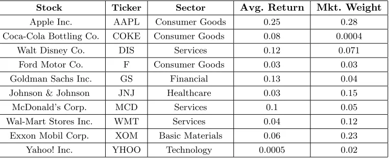
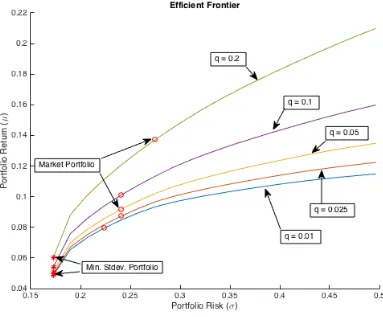
Figure 2.1 Efficient Frontier with and without risk free asset . . . 13
Figure 2.2 Markowitz,N(µ,Σ) vs.N(Π,(1 +τ)Σ) . . . 17
Figure 2.3 Effect of Varyingλ . . . 21
Figure 2.4 Effect of Varyingτ . . . 22
Figure 2.5 Testing Sensitivity of Ω . . . 24
Figure 2.6 Testing Sensitivity ofq . . . 25
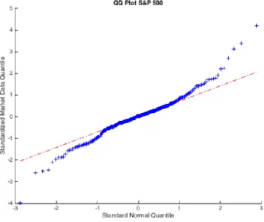
Figure 4.1 S&P 500 Normal Distribution . . . 89
Figure 4.2 S&P 500 Mixed Normal . . . 90
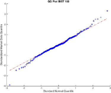
Figure 4.3 BIST 100 Normal Distribution . . . 91
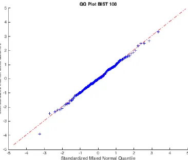
Figure 4.4 BIST 100 Mixed Normal . . . 92
Figure 4.5 Nikkei 225 Normal Distribution . . . 93
Chapter 1
Introduction
Building a portfolio optimization model has three components; defining and estimating the parameters (see Stengel [46] and Lyuu [34]), specifying the objective function (utility function most of the case) and constraints (see for example Steinbach [45] and Kolm et. al. [25]).
First component is the parameter estimation. According to Lyuu [34], we can think about three major parameter estimation techniques; Least Square Method (minimizing the sum of squares of the deviations), Maximum Likelihood Estimator (maximizing the log-likelihood func-tion for all moments) and Methods of Moments (maximizing the log-likelihood funcfunc-tion for some moments). In addition to that some other techniques can be used such as; Bayesian Estimation (see for example Avramov and Zhou [3]) and Inverse Optimization (Ahuja and Orlin [1] and Heuberger [21]). In this thesis we use the Black-Litterman Model which is a combination of the Bayesian framework and Inverse Optimization.
Second component is the objective function. In this thesis, we assume that the purpose of the investors are to maximize the expected return on their portfolios. Therefore the objective function is taken as the expected return of the portfolio. These portfolios are composed of combination of stocks and a risk free asset.
investors are risk averse which means that as the uncertainty on the return increases, investors require more reward. Hence, investors always want to access the uncertainty (i.e. risk). Access-ing the uncertainty is twofold; first a probability distribution should either be assumed or fitted to asset returns, second a tool (risk measure) is needed to measure uncertainty.
Last component is the constraints. In this thesis, we have two constraints; one is related with the risk measure and the other one is related with the asset allocation. An upper bound for the risk measure is given to the model. In addition to that, we require that the sum of all the asset allocations (including the asset allocation to risk free asset) add up to one.
Investors have beliefs and/or information about what is going to happen in the market. However, we assume that it is not possible to use intuitions and/or inside information about the assets or market parameters to beat the market. In other words, we assume the Efficient Market Hypothesis. Moreover, we emphasize that it is impossible to come up with a model such that it predicts the outcome of any random event without an estimation error. The fundamental argument here is that the models are always wrong. This is the direct consequence of their definition and separates models from reality sharply.
All of these arguments stated above are vital atoms of this thesis. Because of the arguments that we have stated, the goal of this thesis is not to beat the market but is to establish a well diversified portfolio using; investor beliefs and historical data available in the market under different settings.
We continue with the Markowitz [29] model, also known as the mean-variance model (MVO).
1.1
Markowitz Portfolio Allocation Problem
Consider a market withnrisky assets. Risky asset returns are denoted by the random vector
r∈Rnwhich is defined on the probability space (Ω,F, P). The mean vector and the covariance
matrix of risky asset returns are denoted byµ=E[r] andΣ∈Rn×nrespectively. The risk free
rate of return is denoted asrf ∈R+∪0. Moreover,x∈Rnis the portfolio weight vector of risky
assets and (1−e0x) is the allocation on the risk-free asset, wheree= (1,1,· · ·,1)0 is a vector of ones in Rn. Moreover, risk aversion coefficient is denoted as; λ(i.e. the amount of risk the
investor is willing to take for a unit of return). The Markowitz Portfolio Allocation Problem is defined as:
Definition 1.1.1 (Markowitz’s PAP).
max
x
µ0x+ (1−e0x)rf −
λx0Σx
2
. (1.1)
shrinkage estimates and bayesian approaches (see Fabozzi Frank J. [13]). Black and Litterman [9] (BLM) also proposes a bayesian approach. Their model, combines the intuitions about the selected assets or market parameters of the investor with the historical information of the market to update the mean vector and covariance matrix. In other words, BLM starts the portfolio allocation problem from the first stage denoted by Markowitz [29].
1.2
Black-Litterman Model (BLM)
We follow the same notation given as in Section 1.1 for the problem parameters and the portfolio allocation vector. Before we state the BLM, we first define the Forward and Inverse Optimization Problems, and give the relationship between inverse optimization and BLM.
1.2.1 Inverse Optimization Problems
Most of the optimization problems in finance are Forward Problems (i.e. Definition 1.2.1). In other words, we maximize (or minimize) an objective function (i.e.f(x;ζ)) over a feasible set (i.e. Γ(ζ)). This set is composed of the problem parameters and the constraints.
Definition 1.2.1 (Forward Problem).
max
x∈Γ(ζ)f(x;ζ), (1.2)
wherex∈Rn.
Definition 1.2.2 (Inverse Problem). Find a value of ζ such that
ˆ
x= argmin
x∈Γ(ζ)
f(x;ζ), (1.3)
wherex∈Rn.
Ahuja and Orlin [1] defines the Inverse Optimization as:“LetS represent a physical system. Assume that we are able to define a set of model parameters which completely define S. All these parameters may not be directly measurable (such as the radius of Earth’s Metallic core). We can operationally define some observable parameters whose actual values hopefully depend on the values of the model parameters. To solve the forward problem is to predict the values of the observable parameters given arbitrary values of the model parameters. To solve the inverse problem is to infer the values of the model parameters from given values of the observable parameters”.
They continue: “A typical optimization problem is a forward problem because it identifies the values of the observable parameters (optimal decision variables), given the values of the model parameters (cost coefficients, right-hand side vector, and the constraint matrix). An inverse optimization problem consists of inferring the values of the model parameters (cost coefficients, right-hand side vector, and the constraint matrix), given the values of observable parameters (optimal decision variables)”.
Moreover, according to Heuberger [21]: “The idea of the inverse optimization is to find values of the parameters which make the known solutions optimum and which differ from the given estimates as little as possible”
According to Ahuja and Orlin [1], Inverse Problems have lot of applications such as: Geo-physical Sciences, Medical Imaging, Traffic Equilibrium and Portfolio Optimization. The Black-Litterman Model uses the inverse optimization to update the expected asset returns.
implied equilibrium return vector, Π, is the customary equilibrium return vector used in the BLM and can be calculated using Inverse Optimization, and is equal to 2λΣxmarket (details
of the derivation is given in Chapter 2). We need estimations for risk aversion coefficient (λ), and covariance matrix (Σ) to use the inverse optimization. In addition to that, a candidate optimal allocation vector is needed. BLM takes market capitalization weights (i.e. xmarket) as
the candidate optimal allocation vector. Moreover, historical covariance matrix is used as the estimation for the covariance matrix. In addition to that,λis fixed subjectively. Furthermore, BLM assumes that investors have views about possible outcomes of the market. This is captured by the view portfolio. This feature of the model is represented as the vector; P. The investor provides the expected return of her view portfolio;q. On the other hand, investor is not certain about the future. Therefore, she provides her uncertainty about the view portfolio (i.e. Ω). In addition to that she is not sure about the estimation of the covariance matrix. Hence, another uncertainty parameter (i.e. τ ∈(0,∞)) is provided.
We give the Canonical Black-Litterman Model under unconstrainted setting next.
Definition 1.2.3 (Black Litterman Model).
max
x
µ0BLx+ (1−e0x)rf −
λx0ΣBLx
2
. (1.4)
where the parameters of the model is given as:
µBL = (τΣ)−1+P0Ω−1P−1 (τΣ)−1Π+P0Ω−1q ,
ΣµBL = (τΣ)−1+P0Ω−1P−1,
ΣBL = Σ+ΣµBL.
Chapter 2
Sensitivity of Inputs in the
Black-Litterman Model
2.1
Introduction
The goal in modern portfolio optimization is to find the optimal portfolio allocation vector given problem parameters, objective function, and constraints. Setting the objective function can be done in many ways. For example, if the investor knows the true (or estimated) value of her risk reward trade off parameter, she can either maximize the unconstrained reward risk trade off optimization problem or minimize the unconstrained risk reward trade off optimization problem. However, estimating the risk reward trade off parameter is difficult. If the investor does not know the true value of her risk reward trade off parameter and cannot get a good estimation for it then, she solves the constrained problem by either setting a lower bound for the reward and minimizing risk or by setting an upper bound for the risk and maximizing reward.
The traditional Markowitz Model uses historical mean returns (µ) and historical covariance matrix (Σ) as inputs to find the optimal portfolio allocation vector. The resulting portfolio, is often not well diversified. Black-Litterman Model (BLM) attempts to fix this problem. BLM assumes that the market is at equilibrium under the Capital Asset Pricing Model (CAPM) and uses inverse optimization to get the implied equilibrium return vector (i.e. Π). Investor views (i.e. q) and Π are used in Bayesian framework to get the posterior distribution for the expected return vector. Hence a better estimate for expected asset returns can be found. The resulting posterior distribution has the updated expected return vector (i.e. µBL) and the updated covariance matrix (i.e. ΣBL). Then, these updated parameters are used in Markowitz
Model to get the optimal portfolio allocation vector. Resulting optimal portfolios usually are more well diversified than the optimal portfolios generated by Markowitz Model (Bertsimas et. al. [7]).
The rest of the chapter is organized as follows. In Section 2.2 we analyze the Markowitz PAP with the risk free asset and without the risk free asset. In Section 2.3 we analyze the parameters of Black-Litterman Model and give the derivation of the implied equilibrium expected return. In Section 2.4 we conclude the chapter.
2.2
Markowitz Portfolio Allocation Problem
We consider a market withnrisky assets. Risky asset returns are denoted by the random vector
r∈Rnwhich is defined on the probability space (Ω,F, P). Vectors are defined as column vectors
unless otherwise stated. The mean vector and the covariance matrix of risky asset returns are denoted byµ=E[r]∈ Rn and Σ∈Rn×n respectively. The risk free rate of return is denoted
as rf ∈ R+∪0. Moreover, x∈ Rn is the portfolio allocation vector of risky assets and xrf is
the allocation to the risk-free asset, wheree= (1,1,· · · ,1)0 is a vector of ones inRn.
Definition 2.2.1 (Markowitz’s PAP without risk free rate).
max
x
µ0x−λx 0Σx
2 :e 0
x= 1
(2.1)
In addition to this model, if a risk-free asset present (i.e.rf ∈R+∪0) in the market. Then one can solve the following PAP.
Definition 2.2.2 (Markowitz’s PAP with risk free rate).
max
x
µ0x+rfxrf −
λx0Σx
2 :e 0
x+xrf = 1
(2.2)
We want our PAP to be as flexible as possible. Hence, if we write the constraint above as:
xrf = (1−e
0
x).
Then we can incorporate this constraint with the objective function and get:
µ0x+rf(1−e0x).
After this transformation we have the same PAP (see Boyd and Vandenberghe [10]) with no constraints:
Definition 2.2.3 (Markowitz’s unconstrained PAP with risk free rate).
max
x
µ0x+rf(1−e0x)−
λx0Σx
2
, (2.3)
Definition 2.2.4 (Minimum variance PAP).
min
x
x0Σx:e0x= 1 . (2.4)
On the other hand, most of the time investors use an upper bond for the portfolio risk in order to control the risk of their portfolios. Let us continue with the constrained Markowitz’s portfolio allocation problem (PAP) (Markowitz [29]):
Definition 2.2.5 (Markowitz’s PAP without risk free rate).
max
x µ
0x
s. t. x0Σx≤L2
e0x= 1
whereL∈R+ is a predefined risk tolerance level of the investor.
We can generate the efficient frontier by setting different values toL (see Figure 2.1). Note that, we assume that short sales are not allowed (i.e.xi ≥0 for all i) when we get the efficient
frontier depicted in Figure 2.1). Moreover, if the risk free rate is present, then we get the following PAP:
Definition 2.2.6 (Markowitz’s PAP).
max
x µ
0
x+ (1−e0x)rf
s. t. x0Σx≤L2
whereL∈R+ is a predefined risk tolerance level of the investor.
runs tangent to the frontier through the point with the highest Sharpe Ratio (i.e. optimal risky portfolio or market portfolio). The portion to the left of the optimal risky portfolio on our adjusted frontier relates to a portfolio where the investor will invest a portion of funds in the risk-free asset. This investment will result in the total risky allocation to be less than one, where the difference is invested in the risk-free asset. The points on the frontier to the right of the optimal risky portfolio are portfolios where the investor will borrow of the risk-free asset to provide additional capital to invest in the portfolio (we assume that risk free rate for borrowing and lending are same). This investment allows the weight of the optimal risky portfolio to be greater than one. Note that the total allocation of the risky and risk free investment always add up to one (also see Figure 2.1).
All of the problems given above can be represented as convex optimization problems. We use a Matlabpackage, ‘cvx’ by [16] to solve these optimization problems numerically.
2.2.1 Obtaining Data
We got historical stock prices for the 10 stocks. We chose the stocks from a variety of sectors over a span of 14 years (Jan. 1, 2000 - Dec. 31, 2013). Selecting stocks from different sectors is the best way to diversify the company based risk (unsystematic risk). The table below lists the stocks we use at this chapter along with their tickers, sectors, average annualized returns, and market capitalization weights. Note that we assume that the risk free rate is 1%.
Table 2.1: Data from Jan. 1, 2000 - Dec. 31, 2013
Stock Ticker Sector Avg. Return Mkt. Weight
Apple Inc. AAPL Consumer Goods 0.25 0.28
Coca-Cola Bottling Co. COKE Consumer Goods 0.08 0.0004
Walt Disney Co. DIS Services 0.12 0.071 Ford Motor Co. F Consumer Goods 0.03 0.03
Goldman Sachs Inc. GS Financial 0.13 0.04
Johnson & Johnson JNJ Healthcare 0.03 0.15
McDonald’s Corp. MCD Services 0.1 0.05
Wal-Mart Stores Inc. WMT Services 0.04 0.12
Exxon Mobil Corp. XOM Basic Materials 0.06 0.23
Yahoo! Inc. YHOO Technology 0.0005 0.02
2.3
Analyzing parameters of Black-Litterman Model
Black-Litterman Model combines investor views with market equilibrium to update the problem parameters. Using the Bayesian framework, BLM estimates the posterior distributions by taking market equilibrium data as the prior distribution and investor views as additional information. For both prior and posterior distributions multivariate normal distribution is assumed. The model assumes that the market is in CAPM equilibrium (see also Sharp [42] [43]). In other words, BLM assumes that every single investor in the market solves the problem given in Definition 2.2.1. The implied equilibrium return vector, Π, is the customary equilibrium return vector used in the BLM and can be calculated using inverse optimization. We need to estimate the risk aversion coefficient (λ) and the covariance matrix (Σ) to use them in the inverse optimization. In addition to that we need a candidate optimal allocation vector. In the BL framework this is given as the market capitalization weights (i.e. xmarket). We give two derivations of Π in
Proposition 2.3.1 and Proposition 2.3.2.
Proposition 2.3.1. Suppose market is in CAPM equilibrium then if the value of the investor risk reward trade off coefficient, λ, is fixed as
µmarket−rf
σ2
market
,
then the adjusted expected return is
Π=λΣxmarket, (2.5)
where Σ is the historical covariance matrix and xmarket is the market weights of the assets
under consideration.
Proof. We assume that the market is CAPM equilibrium, therefore, for all risky assets (i = 1, .., n) we have:
Since, this is true for allifrom 1 ton we have,
µ=rfe+β(µmarket−rf).
where, the value of β is given by
β= Cov(r,r 0x
market)
σmarket2 . Plug the value of βto the above equation and get
µ=rfe+
Cov(r,r0xmarket)
σmarket2 (µmarket−rf). This is nothing but
µ−rfe=Cov(r,r0)xmarket
(µmarket−rf)
σ2
market
.
Then we fix the value ofλas
λ= µmarket−rf σmarket2 . We get the desired result;
Π=λΣxmarket.
This completes the proof.
Now, let us give another way to get the adjusted expected return.
Proposition 2.3.2. Suppose every single investor in the market solves the unconstrained PAP given in Definition 2.2.1 then the value of the adjusted expected return is:
Π=λΣxmarket, (2.6)
whereλis the risk reward trade off coefficient,Σis the historical covariance matrix, andxmarket
Proof. The problem given in Definition 2.2.1 is an unconstrained optimization and can be represented as a convex optimization problem. Therefore, first order necessary condition is also sufficient. Hence, if we take the derivate with respect to the vector x and set the result equal to zero, we have
µ−rfe−λΣx= 0. (2.7)
If we takexmarket as the candidate optimal solution then by the virtue of the inverse
optimiza-tion we get
Π=λΣxmarket. (2.8)
This completes the proof.
Note that as long as we fix the value of the risk reward trade-off as
λ= µmarket−rf σmarket2 ,
then assuming CAPM or PAP given in Definition 2.2.1 does not matter. Estimatingλcan also be subjective. For example, He and Litterman [19] fix λ to 1.25 (the reason for that can be found in their paper).
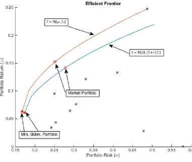
Figure 2.2: Markowitz, N(µ,Σ) vs. N(Π,(1 +τ)Σ)
Let us continue with the other inputs of BLM; the model takes historical data (µ, Σ,
xmarket), view portfolio (P) and it’s value (q), and confidence in these views (Ω,τ) to derive an
updated mean return vector (i.e.µBL), and covariance matrix (i.e.ΣBL). Using BLM investors
can get a portfolio allocation vector based on their view(s). Following He and Litterman [19], the updated parameters can be represented as:
µBL = (τΣ)−1+P0Ω−1P−1 (τΣ)−1Π+P0Ω−1q ,
ΣBL = Σ+ΣµBL (where ΣBLµ = (τΣ)−1+P0Ω−1P
2.3.1 Using Inverse Optimization to Get BLM
In this subsection, we follow the arguments given in Bertsimas et. al. (2012). They show that one can get Black-Litterman type estimations using only Inverse Optimization (see Proposition 2.3.3). They assume that all the investors in the market solve the unconstrained mean variance PAP. Moreover, the candidate optimal solution for the inverse problem is the market weights (i.e.xmarket). They combine the market equilibrium and private information to feed the inverse
model. Hence, the nominal values for the inverse problem are the market weights and the investor view(s) respectively.
Proposition 2.3.3( Proposition 2 of Bertsimas et. al. (2012) ). BLM estimation for the mean vector can be directly found using inverse optimization and it is given as:
µBL=ΣµBL
I P 0
Ω−1τ
Π q (2.9) where,
ΣµBL = I P 0
Ω−1τ
I P −1 , (2.10) Ωτ =
τΣ 0
0 Ω
, (2.11)
and Iis an identity matrix.
Proof. We give sketch of the proof from Proposition 2 of Bertsimas et. al. (2012). Let us define the BLM in the sense of inverse optimization:
min
µ,Σ,t
( t:
µ−rf −2δΣxmkt
Pµ−q
≤t,Σ≥0 )
and, consider this problem under the weighted l2 norm kzkΩτ
2 = q
z0Ω−1
τ z where Σ is fixed.
Then we get;
min µ I P µ− Π q 0
Ω−1τ
I P µ− Π q
. (2.13)
This problem can be represented as:
min µ
Ω−1τ /2
I P µ−Ω
−1/2
τ Π q 2 2 (2.14)
Problem given in (2.14) is nothing but the least squares problem and can be represented as:
min
y kAy−bk. (2.15)
In Equation (2.15)
A=Ω−1τ /2
I P µ, and
b=Ω−1τ /2
Π q .
Closed form solution is given as:
y∗ = (A0A)−1A0b. (2.16)
This is nothing but
µBL=ΣµBL
I P 0
Ω−1τ
Π q
Hence, we get the mean vector of the Black-Litterman Model.
Proposition 2.3.4. Following the same arguments and the notation presented in Proposition 2.3.3, the covariance matrix for the Black-Litterman Model is given as:
ΣBL=Σ+ (A0A)−1.
Proof. Consider the problem
min
y kAy−bk.
The error on the estimation of y is given by (A0A)−1 (by sections E.5 and E.6 of Bertsekas (2005)). Following the same notation presented in Proposition 2.3.3 and the arguments above, we can deriveΣBL:
ΣBL = Σ+E[(y−y∗)(y−y∗)0]
= Σ+ (A0A)−1. (2.17)
This is nothing but
ΣBL=Σ+ΣµBL.
In the following subsections, we analyze the sensitivity of the problem parameters:λ,q,Ω, and τ.
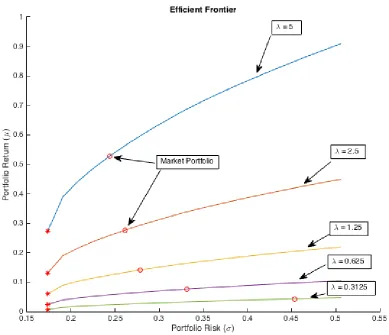
2.3.2 Analyzing the sensitivity of λ
The parameter λ is the risk aversion coefficient. He and Litterman [19] fix it’s value to 1.25. Note thatλis only used when we calculate the value ofΠ(i.e. the implied equilibrium return vector).
Consider the PAP given in Definition 2.2.6 and assume that short sales are not allowed (i.e. xi ≥ 0 for all i). In addition to that suppose the investor does not have any view. Then, an
Figure 2.3: Effect of Varyingλ
2.3.3 Analyzing the sensitivity of τ
The parameter τ represents the level of uncertainty an investor holds in the prior distribution. There is no convention in the literature about how to estimate the value of τ. For instance, Black and Litterman [9] says thatτ should be close to 0 while Satchell and Scowcroft [40] states that τ should be closer to 1. Some authors, such as Meucci [30], have even proposed a model without the useτ to avoid this discrepancy (this model known as the Alternate Model).
that as the investor uncertainty gets larger, the posterior covariance matrix goes to (1 +τ)Σ. If that is case then, as τ gets closer to 0, then the posterior covariance becomes the historical covariance. Hence the BL efficient frontier converges to that of the mean variance model with updated µ(i.e. Π). Moreover, as τ increases from 0, uncertainty about our prior distribution increases, and thus, increases our risk due to the additional uncertainty. The effect ofτ on the BL efficient frontier is a horizontal shift that moves efficient frontier right asτ increases. Our intuition is that the BL efficient frontier illustrates a horizontal shift of the constrained portfolio allocation problem with r ∼ N(Π,Σ) efficient frontier by a scale of √1 +τ. This movement can be seen in Figure 2.4.
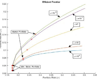
2.3.4 Analyzing the sensitivity of Ω
The Ωenables investors to state their level of uncertainty about their views. If investor has k views then,Ωis ak×k diagonal matrix where the level of uncertainty in each view is stated. Estimating the value of Ω is another challenge for the use of this model. Hence, He and Litterman [19] use the following idea to fix the value of the uncertainty matrix:
Ω=ωτP0ΣP. (2.18)
Figure 2.5: Testing Sensitivity of Ω
2.3.5 Analyzing the sensitivity of q
Figure 2.6: Testing Sensitivity ofq
2.4
Conclusion
efficient frontier horizontally shifts; as ω increases the investor is less and less confident in the views, and BL efficient frontier moves towards the MVO model efficient frontier adjusted for the given τ and Π; as the values inqincreases the efficient frontier gets bigger.
Chapter 3
Closed-Form Solutions for
Black-Litterman Models with
Conditional Value at Risk
3.1
Introduction
opti-mization problem (see Meucci [30] and Fabozzi et. al. [13]). Because of the reasons stated above, Markowitz’s optimal allocation vectors are lack of diversification and/or has corner solutions.
Black-Litterman Model (BLM) [9] proposes a parameter estimation technique in which the investor’s view can be integrated with the historical performance to estimate the problem parameters. There are two different ways to approach this model in the literature; the original model (canonical model) and the later one (alternate model).
Canonical model combines the intuitions about the selected assets or asset classes of the investors with the historical information of the market in order to update the mean vector and covariance matrix. This is done by using the bayesian framework. BLM assumes that the expected returns are random variables themselves. These random variables are normally dis-tributed and centered at the CAPM equilibrium returns with historical covariance matrix. BLM considers CAPM equilibrium returns as the prior distribution of the asset returns. Furthermore, investors have views on the assets (or asset classes) in the market and take the CAPM equilib-rium as the reference point to specify their view(s). Those views are the additional information to the bayesian framework. On other hand, in the alternate model, market factors are consid-ered instead of asset returns. In addition to that, the expected value of the market factors are not random variables (see also Walters [47] and Meucci [30]). Both models, use the updated parameters in the mean-variance framework to get the optimal portfolio allocation vector. In-vestor view(s) has two forms; relative view(s) (the sum of the weights of views add up to zero) and absolute view(s) (there is only one asset in this form of view, therefore, that asset’s weight is always equal to one). Some of the authors use market capitalization weights when specifying the views (i.e. He and Litterman [19] and Idzorek T. [22]). On the other hand, some of them such as Meucci A. [31] and Satchell and Scowcroft [40] use an equal weighted scheme.
is given by Xiao and Valdez [48] (see also Proposition 3.5.1). Although, CVaR has become more and more popular as a coherent risk measure in the financial industry, derivation of the optimal solution analytically is extremely difficult under CVaR constraint. Hence, we propose an efficient approximation algorithm for optimization problems with CVaR constraint. Then, based on the approximation algorithm, we derive the closed-form solutions for the BLM with elliptical distributions and CVaR. To our best knowledge, no closed-form solutions for BLM with CVaR have been derived before.
3.2
Portfolio Allocation Problem (PAP)
We consider a market withnrisky assets. Risky asset returns are denoted by the random vector
r∈Rnwhich is defined on the probability space (Ω,F, P). Vectors are defined as column vectors
unless otherwise stated. The mean vector and the covariance matrix of risky asset returns are denoted by µ = E[r]∈ Rn and Σ ∈ Rn×n respectively. We assume that µ is finite, and Σ is
finite and positive definite. The risk free rate of return is denoted as rf ∈ R+∪0. Moreover,
x ∈ Rn is the portfolio weight vector of risky assets and (1−e0x) is the allocation on the risk-free asset, wheree= (1,1,· · ·,1)0 is a vector of ones inRn.
First we define the space of portfolio returns for a given number of available risky assets and a risk-free asset.
Definition 3.2.1 (Space of Portfolio Returns).
V ={˜v∈R:∃(rf,x) s.t. ˜v=v0+ (r−µ)0x} (3.1)
where v0=µ0x+ (1−e0x)rf.
Note that in Definition 3.2.1 each portfolio return is represented as a combination of return with certainty (i.e. µ0x+ (1−e0x)rf) and return with uncertainty (i.e. (r−µ)0x).
Proof. Let ˜v1∈ V, ˜v2 ∈ V and γ ∈Rs.t. 0≤γ ≤1. Let ˜v3 ≡γ˜v1+ (1−γ)˜v2. Then,
˜
v3 =γ˜v1+ (1−γ)˜v2
=γ(v10+z0x1) + (1−γ)(v02+z0x2) (wherez=r−µand x1,x2 ∈R) =γv01+ (1−γ)v02+γ(z0x1) + (1−γ)(z0x2)
=v03+γ(z0x1) + (1−γ)(z0x2) (where v30 =γv10+ (1−γ)v20) =v03+z0 γx1+ (1−γ)x2
=v03+z0x3 (where x3=γx1+ (1−γ)x2)
Hence, ˜v3 ∈ V, therefore,V is a convex set.
Definition 3.2.2 (Affine Function). Letz=r−µand x∈Rn,v
0 ∈R. Then, every function
of the form
f(x) =v0+hz,xi
is an affine function by Theorem 4.1 of Rockafellar [36].
Let us continue with the definition of the constrained Markowitz’s portfolio allocation prob-lem (PAP) (Markowitz [29]):
Definition 3.2.3 (Markowitz’s PAP).
max
x {µ
0
x+ (1−e0x)rf :
√
x0Σx≤L}, (3.2)
whereL∈R+ is a predefined risk tolerance level of the investor.
In Markowitz’s PAP, the variance is used as the risk measure. There are other risk measures that are widely used, such as value at risk (VaR) and conditional value at risk (CVaR).
the random variable with confidence levelα is,
V aRα(Y) = inf{y∈R:P(y + Y≤0)≤1−α}. Definition 3.2.5 (PAP with VaR).
max
x {µ
0
x+ (1−e0x)rf :V aRα((r−rfe)0x+rf)≤L} (3.3)
V aRα is not a coherent risk measure (see Artzner et. al. [2]). In particular, diversification
benefit may not be present under VaR. On the other hand, CVaR is coherent (properties of CVaR can be found in Rockafellar and Uryasev [37] and [38]). This is the main reason that CVaR is a very popular risk measure. CVaR sometimes called as mean short fall or tail-VaR as well. Although, their definitions are different, they give the same result under continuous random variables (Krokhmal et. al. [26]).
Definition 3.2.6 (CVaR). Given α ∈ (0,1) and a random variable (i.e. Y) the conditional value at risk of the random variable with confidence level α is,
CV aRα(Y) =−E[Y|Y≤ −V aRα(Y)].
Here we consider the PAP with CVaR:
Definition 3.2.7 (PAP with CVaR).
max
x {µ
0x+ (1−e0x)r
f :CV aRα((r−rfe)0x+rf)≤L}. (3.4)
Definition 3.2.8 (GPAP with generic coherent risk measure ρ).
max
x {µ
0
x+ (1−e0x)rf :ρ((r−rfe)0x+rf)≤L} (3.5)
We want to solve the PAP given in Definition 3.2.7. CVaR is a coherent risk measure so we can use results from Natarajan et. al. [32] to find the robust counterpart of the CVaR constraint (with elliptical uncertainty sets to be specified below). In other words, we can convert the GPAP with generic coherent risk measure given in Definition 3.2.8 to the GPAP with robust optimization given in Definition 3.2.9 (see below) if a certain condition holds and vice versa (see Natarajan et. al. [32]). The closed form solution of the robust optimization with elliptical uncertainty sets are available as we mention below. Moreover, if we assume an elliptical distribution then we can get the closed form representation of CVaR (see Proposition 3.3.4 below).
We can use uncertainty sets in order to model the return with uncertainty (i.e. (r−µ)). In particular, we use elliptical uncertainty sets:
Uβ ={r−µ: (r−µ)0Σ−1(r−µ)≤β2}
where β is the scaling parameter which models the risk averseness of the investor from the deviation of the realized returns from their forecasted values.
The reasons of using elliptical uncertainty sets is twofold: First, when uncertainty set is elliptical then the robust programming can be converted into conic programming and the closed form solution exist (Ben Tal and Nemirovski [5]); second, elliptical uncertainty sets can be used for leptokurtic behavior of asset returns.
Definition 3.2.9 (GPAP with robust optimization).
max
x {µ
0
x+ (1−e0x)rf : (r−rfe)0x+rf ≥ −L∀r−µ∈ Uβ }
The process of finding the robust counterpart is straight forward. We first start with defining the robust counterpart risk measure, ηUβ(˜v), given by Natarajan et. al. [32] and it can be
represented as:
ηUβ(v0+ (r−µ)
0
x) =− min
r−µ∈Uβ
(v0+ (r−µ)0x) (3.6)
Definition 3.2.10. The PAP with robust counterpart risk measure is given by
max
x {µ
0
x+ (1−e0x)rf :ηUβ (r−rfe)
0
x+rf
≤L}
Let us show that problems given in Definitions 3.2.9 and 3.2.10 are the same problems. We are interested with the representation of the constraint, therefore, we consider the constraint given in Definition 3.2.9. In other words, we are interested in
(r−rfe)0x+rf ≥ −L ∀r−µ∈ Uβ .
This can be written as:
(rfe−r)0x−rf ≤L ∀r−µ∈ Uβ
⇔ −(r−µ)0x−µ0x+ (1−e0x)rf ≤L ∀r−µ∈ Uβ
⇔ max
r−µ∈Uβ
−(r−µ)0x−µ0x−(1−e0x)rf
≤L
⇔ max
r−µ∈Uβ
− (r−µ)0x+µ0x+ (1−e0x)rf
⇔ − min
r−µ∈Uβ
(r−µ)0x+µ0x+ (1−e0x)rf
≤L
⇔ηUβ µ0x+ (1−e0x)rf + (r−µ)0x
≤L
⇔ηUβ (r−rfe)0x+rf
≤L.
Proposition 3.2.2. If an elliptical uncertainty set is assumed in the constraint of the PAP given in Definition 3.2.9 then this PAP can be represented as:
max
x {µ
0x+ (1−e0x)r
f :− µ0x+ (1−e0x)rf
+β
√
x0Σx≤L}
Proof. Let us start with considering the constraint of the PAP given in Definition 3.2.9, in other words,
(r−rfe)0x+rf ≥ −L∀r−µ∈ Uβ.
Note that this constraint is nothing but:
ηUβ µ0x+ (1−e0x)rf + (r−µ)0x
≤L.
We can use Equation (3.6) to get
ηUβ(v0+ (r−µ)
0x) =− min
r−µ∈Uβ
(v0+ (r−µ)0x)
wherev0 =µ0x+ (1−e0x)rf. We are minimizing an affine function,
(r−µ)0x+µ0x+ (1−e0x)rf
,
the closed form solution is given by Ben Tal and Nemirovski[6]:
min
r−µ∈Eβ
(v0+ (r−µ)0x) =v0−β √
x0Σx. (3.7)
Therefore,
−
min
r−µ∈Eβ
(v0+ (r−µ)0x)
=−v0+β √
x0Σx.
Hence,
ηU
β(v0+ (r−µ)
0x) =−v 0+β
√
x0Σx
Use value ofv0 and get the desired result.
Before we proceed, we would like to state some results when we assume multivariate normal distribution for return vector for PAP with VaR and CVaR. The proposition stated below gives a close form solution for VaR risk measure, defined on Definition 3.2.4, if a multivariate normal distribution is assumed for the asset returns.
Proposition 3.2.3. Let the asset return distribution, r ∈ Rn, follows a multivariate normal
distribution with mean µ and covariance matrix Σ (i.e. r ∼ N(µ,Σ)) and x be the weight distribution of the risky assets. Then
V aRα((r−rfe)0x+rf) =−(x0µ+ (1−e0x)rf) +z1−α
√
x0Σx.
Proof. Let us start with considering a standard normal random variable (i.e. ˜v∼N(0,1)). Note that ˜v is one dimensional. Now, suppose that the portfolio return distribution can be modeled as ˜v. (i.e. portfolio return∼N(0,1)). Then we have
by definition of VaR. Next, suppose that ˜v∼N(µ, σ2). Then, it is easy to show that
V aRα(x) =−µ+z1−ασ
by using the definition of VaR and cumulative normal distribution. Next, let us consider the portfolio return distribution in a multidimensional space. If we replaceµ andσ with the mean of the portfolio and standard deviation, respectively. Then we get:
V aRα(x) =−(µ0x+ (1−e0x)rf) +z1−α
√
x0Σx
Next, we give the closed form representations of CVaR when asset returns are multivariate normal.
Proposition 3.2.4. Let the asset return distribution, r ∈ Rn, follows a multivariate normal
distribution with meanµand covariance matrixΣ(i.e. r∼N(µ,Σ)). Then
CV aRα((r−rfe)0x+rf) =−(µ0x+ (1−e0x)rf) +
f(z1−α)
1−α √
x0Σx.
Proof. Let ˜v be a standard normal random variable (i.e. ˜v ∼ N(0,1)). Furthermore, suppose this is the distribution of the portfolio return. ThenCV aRα(˜v) can be represented as follows,
CV aRα(˜v) =−
R−z1−α
−∞ vf˜˜ v(˜v)d˜v 1−α
(where z1−α=V aRα(˜v))
=− R−z1−α
−∞ vf˜ ˜v(˜v)d˜v F(−z1−α)
=−
Z −z1−α
−∞ ˜ v√1
2πexp
−v˜ 2 2
d˜v
.
= Z ∞
z2 1−α
1 2√2πexp
−u
2
du .
F(−z1−α)
(make substitutionu= ˜v2)
=f(z1−α)
.
F(−z1−α).
Now, suppose that y∼N(µy, σy2). Hence,
CV aRα(y) =−E[y|y < µy−z1−ασy]
(sincey∼N(µy, σy) and z1−α=V aRα(y))
=−E[µy+σyx|µy+σyx < µy−z1−ασy] (where x= (y−µy)/(σy) )
=−µy−σyE[x|µy+σyx < µy−z1−ασy]
=−µy−σyE[x|x <−z1−α]
=−µy+σy
f(−z1−α)
F(−z1−α)
(since ˜v∼N(0,1))
=−µy+σy
f(z1−α)
1−α . (since ˜v∼N(0,1))
Replace µy and σy with the mean of the portfolio and standard deviation, respectively. Then
we get;
CV aRα((r−rfe)0x+rf) =−(µ0x+ (1−e0x)rf) +
f(z1−α)
1−α √
Now, we first state and give the proof of a proposition by Bertsimas D., Gupta V., Paschalidis Ioannis Ch.(2012) [7] to give an introduction to the relationship between uncertainty sets and risk measures.
Proposition 3.2.5. Consider the following uncertainty sets:
U1 ={r−rfe: (r−rfe)0Σ−1(r−rfe)≤1}, (3.8)
Uz1−α ={r−µ: (r−µ)0Σ−1(r−µ)≤z1−2 α} (3.9)
(i) Problem given in Definition 3.2.9 with U =U1 is equivalent to the Markowitz problem.
(ii) If r is distributed as a multivariate Gaussian, r ∼ N(µ,Σ) then Definition 3.2.9 with U =Uz1−α is equivalent to the PAP with Value at Risk (3.3).
Proof. (i) Note that the objective functions of the problems are same, therefore, we shall focus only on the constraint. Let us define the robust counterpart risk measure of the general portfolio allocation problem (3.7).
ForU =U1 we have:
ηU1(v0+ (r−µ)0x) =ηU1 rf + (r−rfe) 0x
=− min
r−rfe∈U1
(rf + (r−rfe)0x) (by equation (3.6))
=−rf+ 1
√
x0Σx (by equation (3.7)).
Therefore the risk constraint turns into;
−rf+
√
this is nothing but
√
x0Σx≤L1,
whereL1 =L+rf.
(ii) Note that the objective functions of the problems are same, therefore, we shall focus only on the constraint on risk constraint. So that,
ηUz1−α(v0+ (r−µ)
0x) =ηU
z1−α µ
0x+ (1−e0x)r
f + (r−µ)0x
=− min
r∈Uz1−α
µ0x+ (1−e0x)rf + (r−µ)0x
by equation (3.6)
=− µ0x+ (1−e0x)rf
+z1−α
√
xΣx by equation (3.7)
=V aRα (r−rfe)0x+rf
by Proposition 3.2.3
3.3
GPAP with Elliptical Distributions
In this section, we give the relationship between GPAP with robust optimization under some elliptical uncertainty sets and PAP with CVaR under some well known multivariate elliptical distributions (for details on elliptical distributions please see Fang et. al. [14]). Let us begin with the definition of elliptical distributions.
Definition 3.3.1 (Elliptical Distributions). Let r be the n dimensional asset return vector with the following density
fr(r;µ,D) =|D|−
1
whereµis a location vector, D is an positive definite dispersion matrix andgn(.) is the
distri-bution specific density generator function. We use the notation r∼EDn(µ,D, gn). Moreover,
if the density defined on equation (3.10) exist then it satisfies the following equation,
Z ∞
0
un2−1gn(u)du= Γ(n/2)
Πn/2 . (3.11)
Interested readers can check the paper by Xiao and Valdez 2013 [48] to see how well known multivariate elliptical distributions are represented by (3.11).
Lemma 3.3.1. (Lemma 4.1 in Xiao and Valdez (2013) [48]) Let v ∼ ED(µ,D, gn) and let
x∈Rn then,
CV aRα(r0x) =−x0µ+CV aRα(Y)(
√
x0Dx) (3.12)
whereY ∼ED1(0,1, g1) i.e. a spherical random variable. Moreover,
CV aRα(Y) =
1 1−αG¯
y2 1−α
2
(3.13)
where
¯
G(x) =G(∞)−G(x) ifG(∞)<∞
such that
G(x) = Z x
0
g1(2u)du,
and y1−α satisfies
FY(y1−α) =
Z y1−α
−∞
g1(u2)du= 1−α (3.14)
Proof. Please see Xiao and Valdez (2013) [48].
Proposition 3.3.2. Letr∼t(µ,D, m) and letx∈Rn then equation (3.13) becomes
CV aRα(Y) =
c2m (1−α)(m−1)
1 +y
2 1−α
m
1−m
2 ,
where
c2 =
(πm)−1/2Γ ((m+ 1)/2) Γ (m/2) .
Proof. We use the definitions of G(∞) and G(y21−α/2) from Lemma 3.3.1. Let us start with calculating G(∞):
G(∞) = Z ∞
0
g1(2u)du
= Z ∞
0 c2
1 +2u
m
−(1+m) 2 du = c2m 2 Z ∞ 1
v−(1+2m)dv (make substitution (1 + 2u/m=v))
=− c2m
1−m. (3.15)
Next, we calculate G(y1−2 α/2), G(yα2/2) =
Z y12−α/2 0
g1(2u)du
=
Z y12−α/2
0
c2
1 +2u m
−(1+2m) du
= c2m 2
Z 1+y12−α/m 1
= c2m 1−m
1 +y
2 1−α
m
(1−m)/2 −1
!
. (3.16)
Now, using equations (3.15) and (3.16) we get
CV aRα(Y) =
1 (1−α)
− c2m
1−m − c2m 1−m
1 + (y21−α/m)(1−m)/2−1
= 1 (1−α)
c2m m−1
1 +y
2 1−α m 1 −m 2 .
Proposition 3.3.3. Letr∼M L(µ,D) and let x∈Rn then equation (3.13) becomes
CV aRα(Y) =
c3 2(1−α)
1− 1 1 +e−y12−α
,
where
c3 =
Γ(n/2) π1/2
Z ∞
0
un/2−1 e −u
(1 +e−u)2du −1
.
Proof. Note that definitions ofG(∞) and G(y21−α/2) are given in Lemma 3.3.1. We start with
calculating G(∞):
G(∞) = Z ∞
0
c3 e −2u
(1 +e−2u)2du
= Z 1
2 c3
−2x2du (make substitution (1 +e
−2u =x))
= c3
Next, we calculate G(y1−2 α/2), G(yα2/2) =
Z y12−α/2 0
c3
u−2u (1 +e−2u)2du
=
Z 1+e−y 2 1−α
2
c1
−2x2du (make substitution (1 +e
−2u =x))
=c3 −
1 2 +
1 1 +e−y21−α
. (3.18)
Now, combine equations (3.17) and (3.18) we get
CV aRα(Y) =
1 (1−α)
c1 4 − c1 2 − 1 2 + 1 1 +e−y12−α
= c3 2(1−α)
1− 1 1 +e−y21−α
We give the connection between GPAP with generic risk measure and GPAP in the sense of robust optimization in the following proposition. Note that we use CVaR as our coherent risk measure.
Proposition 3.3.4 (CVaR and Uncertainty Sets). Consider the following uncertainty set:
Uβα ={r−µ: (r−µ)0Σ−1(r−µ)≤βα2}, (3.19) (i) if r∼N(µ,Σ) and
βα =f(z1−α)/(1−α),
wheref(·) is the standard normal density function andz1−α is the z-score,
the degree of freedom, and
βα =
c2m (1−α)(m−1)
1 +y
2 1−α
m
1−m
2 ,
where
c2 =
(πm)−1/2Γ ((m+ 1)/2) Γ (m/2) , andy1−α satisfying equation (3.14),
(iii) if rfollows a multivariate Logistics distribution i.e.r∼M L(µ,Σ), and
βα =
c3 2(1−α)
1− 1 1 +e−y21−α
,
where
c3=
Γ(n/2) π1/2
Z ∞
0
un/2−1 e −u
(1 +e−u)2du −1
,
andy1−α satisfying equation (3.14),
then we get the PAP with CVaR for multivariate Normal, Student-t, and Logistics distributions, respectively.
Moreover, the closed-form solution of CVaR is:
CV aRα(˜v) =−(µ0x+ (1−e0x)rf) +βα
√
x0Σx. (3.20)
Proof. For all three cases, we start with the using Theorem 4 of [32] to get the robust counterpart risk measure of a coherent risk measure and give the representation of CVaR (i.e. (3.20)).
(i)
ρ(v0+r0x) =ηUβα(v0+r
0
x)
=ηUβα µ
0
x+ (1−e0x)rf + (r−µ)0x
(by Definition 3.2.1)
=− min
r−µ∈Uβα µ 0
x+ (1−e0x)rf + (r−µ)0x
(by Equation (3.6))
=− µ0x+ (1−e0x)rf
+βα
√
x0Σx
(by equation (3.7))
=CV aRα((r−rfe)0x+rf).
(by Proposition 3.2.4)
(ii)
ρ(v0+r0x) =ηUβα(v0+r
0x)
(by Theorem 4 of [32])
=ηUβα µ
0x+ (1−e0x)r
f + (r−µ)0x
(by Definition 3.2.1)
=− min
r−µ∈Uβα
µ0x+ (1−e0x)rf + (r−µ)0x
(by Equation (3.6))
=− µ0x+ (1−e0x)rf
+βα
√
(by equation (3.7))
=CV aRα((r−rfe)0x)−rf
(by Lemma 3.3.1 and Proposition 3.3.2)
=CV aRα((r−rfe)0x+rf).
(since CVaR is a coherent risk measure)
(iii)
ρ(v0+r0x) =ηUβα(v0+r
0
x)
(by Theorem 4 of [32])
=ηUβα µ
0
x+ (1−e0x)rf + (r−µ)0x
(by Definition 3.2.1)
=− min
r−µ∈Uβα µ 0
x+ (1−e0x)rf + (r−µ)0x
(by Equation (3.6))
=− µ0x+ (1−e0x)rf
+βα
√
x0Σx
(by equation (3.7))
=CV aRα((r−rfe)0x)−rf.
=CV aRα((r−rfe)0x+rf).
(since CVaR is a coherent risk measure)
Note that one can also use multivariate elliptical distributions directly and come up with the corresponding βα values (see Landsman and Valdez [28]). For part (i) see also Bertsimas
et. al. [7] and references there in.
3.4
CVaR Approximation
Consider the general constrained portfolio optimization problem (i.e. Definition 3.2.9) with uncertainty set given by (3.19). Then by using Proposition 3.3.4 we get the Lagrangian function of the optimization problem:
L(x, δ) =µ0x+ (1−e0x)rf−
CV aRα (r−rfe)0x+rf
−Lδ
=µ0x+ (1−e0x)rf−
−(µ0x+ (1−e0x)rf) +βα
√
x0Σx−L
δ
=(1 +δ)(−µ0x−(1−e0x)rf)−δ
βα
√
x0Σx−L.
Now, take the partial derivative with respect to xto get the first order necessary condition.
(1 +δ) (µ−erf)−δ
βα(x0Σx)−1/2Σx
= 0.
of the optimal solution for that problem.
The asset return distribution is assumed to be elliptical with the parameters defined in Proposition 3.5.1. Furthermore, historical mean vector and covariance matrix are taken as the mean of the asset returns and covariance matrix, respectively. We can rewrite the constraint as (using Proposition 3.3.4)
CV aRα((r−rfe)0x+rf)≤L (3.21)
⇔ −(µ0x+ (1−e0x)rf) +βα
√
x0Σx≤L
⇔√x0Σx≤ (L+µ
0x+ (1−e0x)r
f)
βα
.
Let
˜
L(x)≡ (L+µ
0x+ (1−e0x)r
f)
βα
. (3.22)
Before we proceed to the main results we define the risk-adjusted return vector:
˜
µ=Σ−1/2(µ−erf).
Note that ˜µis finite.
To solve the PAP with CVaR, we use an approximation approach. First, we define the feasible solution spaceP as
P ≡ {x∈Rn:CV aRα((r−rfe)0x+rf)≤L}. (3.23)
Next, we define a sequence of vectors {xn}n≥0 as follows:
xn+1= arg max
x {µ
0x+ (1−e0x)r
f :
√
x0Σx≤L(˜ xn)}, n≥0. (3.25) In other words, xn+1 is the solution of the following PAP
max
x {µ
0x+ (1−e0x)r
f :
√
x0Σx≤L(˜ xn)}. (3.26) We want to point out that the initial vector x0 can be any vector in P. For example, we can choose x0 =0. More details will be given in Proposition 3.4.2. As we can see, the above PAP is of Markowitz mean-variance type, and it is very easy to solve.
We have the following results.
Lemma 3.4.1. Let{xn}n≥0 be given by (3.24)-(3.25). Then xn∈ P, ∀n≥0 and {L(˜ xn)}n≥0 is a non-decreasing sequence.
Proof. We prove the result by induction. First, from (3.24), we see that x0 ∈ P. Further, by virtue of (3.23) and (3.21), it is easy to check thatpx00Σx0≤L(˜ x0). By virtue of the definition of x1 (see (3.25)), we can get that
µ0x0+ (1−e0x0)rf ≤µ0x1+ (1−e0x1)rf.
Then, by the definition of ˜L(x) (3.22), we have
˜
L(x0)≤L(˜ x1).
Using the definition of x1 (see (3.25)) and the above inequality, we have that
q
x01Σx1 ≤L(˜ x0)≤L(˜ x1).
same argument as we used for x0 and x1, we can show that
xn+1 ∈ P, L(˜ xn)≤L(˜ xn+1).
This completes the proof.
Unlike the classical mean-variance optimization problem which always have a solution, the PAP with CVaR may not have a bounded solution. For example, ifn= 1, the CVaR constraint becomes−(µ−rf)x−rf+βασx≤L, which might become redundant whenµ−rf > σβα, and
the optimal solution is x=∞. Therefore, some extra conditions are needed for the PAP with CVaR to be well-defined.
Define the risk-adjusted return vector ˜µand a constantdas
˜
µ≡Σ−1/2(µ−erf), (3.27)
d≡ q
(µ−erf)0Σ−1(µ−erf). (3.28)
It is easy to see thatd=kµ˜k. We assume the following condition holds:
βα−d >0. (3.29)
This condition is not a strong condition and it would usually hold. Note that as explained above, if it doesn’t hold, the solution is trivial. Hence, condition (3.29) doesn’t really constrain α. For example, forn= 1 with normal distributions,βα= 2.0627 for α= 95% anddis nothing
but the Sharp Ratio of the risky asset. Assume that µ= 20%, rf = 0% and σ = 16%, we can
getd= (µ−rf)/σ= 1.25. Note that the risk-reward trade off is usually taken as δ= 1.25 (see
Proposition 3.4.2 (Conv. of ˜L(xn)). Assume that (3.29) holds and define
˜
L∗ ≡ L+rf βα−d
. (3.30)
Let{xn}n≥0 be given by (3.24)-(3.25). Then we have ˜
L(xn)≤L˜∗, ∀n≥0, (3.31)
and lim
n→∞ ˜
L(xn) = ˜L∗, ∀x0 ∈ P. (3.32) Further, we have
˜
L(x)≤L˜∗, ∀x∈ P. (3.33)
Proof. By virtue of the definition ofxn+1(see (3.25)), we know thatxn+1is the optimal solution of (3.26).The closed-form solution of this problem is well-known:
xn+1 =
Σ−1(µ−erf)
2δ , (3.34)
where δ is the Lagrange multiplier given by δ = d
2 ˜L(xn) and d is defined by (3.28). So we can
get
xn+1 = ˜ L(xn)
d Σ −1
(µ−rfe). (3.35)
Using the definition of ˜L(·), we have
˜
L(xn+1) =
L+rf
βα
+(µ−rfe) 0x
n+1 βα
. (3.36)
It is easy to verify that (3.35) and (3.36) imply
˜
L(xn+1) =
L+rf
βα
+dL(˜ xn) βα
By virtue of Lemma 3.4.1, we have that ˜L(xn+1)≥L(˜ xn). So
L+rf
βα
+d ˜ L(xn)
βα
≥L(˜ xn),
which is equivalent to
˜ L(xn)≤
L+rf
βα−d
.
This holds for anyn≥0. Therefore, (3.30) holds.
Further, by virtue of the recursive formula (3.37), we can get
˜ L(xn) =
L+rf
βα n−1 X j=0 d βα j + d βα n ˜
L(x0). (3.38)
By virtue of (3.29), we know that
d βα <1. Therefore, lim n→∞ ˜ L(xn) =
L+rf
βα
1 1−βd
α
= L+rf βα−d
= ˜L∗,
and it is true for anyx0 ∈ P. Therefore, (3.32) holds.
Finally, for any x ∈ P, we can take x0 = x in (3.24). Then by (3.31), we can get (3.33). This completes the proof.
Now we can present the main result of this section.
Theorem 3.4.3. Assume that (3.29) holds. Then x∗ is an optimal solution to the PAP with CVaR (i.e. problem given by Definition 3.2.7) if and only if ˜L(x∗) = ˜L∗ and x∗ ∈ P, where
˜
L(·),L˜∗ and P are defined by (3.22), (3.30) and (3.23), respectively.
Proof. Define ˆxas a solution of
max
x {µ
0x+ (1−e0x)r
f :
√
Let {xn}n≥0 be given by (3.24)-(3.25). By virtue of (3.31), we know that ˜L(xn) ≤L˜∗. Then,
by virtue of (3.39) and (3.25), we can get that
µ0xn+1+ (1−e0xn+1)rf ≤µ0ˆx+ (1−e0xˆ)rf.
By the definition of ˜L(·) (see (3.22)), we can get ˜L(xn+1)≤L(ˆ˜ x), ∀n≥0, which implies that
˜
L∗ = lim
n→∞ ˜
L(xn)≤L(ˆ˜ x). (3.40)
Since ˆxis a solution of (3.39), the above equation implies that
p ˆ
x0Σxˆ ≤L(ˆ˜ x). (3.41)
Then, using (3.21), we can get that ˆx∈ P. Now by virtue of (3.33), we know that
˜
L(ˆx)≤L˜∗.
Together with (3.40), the above inequality implies that
˜
L(ˆx) = ˜L∗. (3.42)
Let x∗ be an optimal solution of the PAP with CVaR:
x∗∈argmax{(µ−e)0x+rf :CV aRα((r−rfe)0x+rf)≤L}.
Then we have x∗ ∈ P. Based on (3.41), we know that ˆx∈ P. Sincex∗ is the optimal solution, we must have
which implies
˜
L(ˆx)≤L(˜ x∗).
Now, takingx0 asx∗ and using Lemma 3.4.1, we can get that
˜
L(x∗)≤L˜∗= ˜L(ˆx).
Therefore, we must have ˜L(x∗) = ˜L(ˆx) = ˜L∗.
On the other hand, if there is an x∗ ∈ P such that ˜L(x∗) = ˜L∗, then we can use (3.33) to derive that x∗ maximizes ˜L(·) over P. By the definition of ˜L(x) (see (3.22)), we can see that maximizing µ0x+ (1−erf)xis equivalent to maximizing ˜L(x). Therefore, x∗ maximizes
µ0x+ (1−e0x)rf overP and it is an optimal solution of the PAP with CVaR given by Definition
3.2.7. This completes the proof.
Another important result in this section is the following Theorem.
Theorem 3.4.4(Conv. of ˜L(xn) ). L(˜ xn) n→∞
−−−→L(˜ x∗) wherex∗ is the optimal solution to the PAP with CVaR (i.e. problem given by Definition 3.2.7).
Proof. From Proposition 3.4.2, we know that the sequence{L(˜ xn)}converges to a real number
(i.e. ˜L∗). We will show that ˜L∗= ˜L(x∗). Define ˆxas the solution of
max
x {µ
0
x+ (1−e0x)rf :
√
x0Σx≤L˜∗}. (3.44)
The closed form solution to this problem is well known:
ˆ
x= ˜ L∗
d Σ −1
(µ−rfe). (3.45)
Using (3.22) we can get
˜
L(ˆx) = L+ (µ−erf) 0xˆ+r
f
βα
Using equations (3.45) and (3.46) we get
˜
L(ˆx) = L+ ˜L ∗d+r
f
βα
Since
˜
L∗ = L+rf βα−d
by Proposition 3.4.2, we get
˜
L(ˆx) = L+
L+rf
βα−dd+rf
βα
=
(L+rf)(βα−d+d)
βα−d
βα
= L+rf βα−d
= L˜∗.
Therefore,
˜
L(ˆx) = ˜L∗. (3.47)
On the other hand, by definition, we have
x∗∈argmax{(µ−e)0x+rf :CV aRα((r−rfe)0x+rf)≤L}.
Further, the constraint should be binding for the optimal solution, so we can getCV aRα((r−
rfe)0x∗+rf) =L. By the definition of ˜L(see (3.22)), we can get
CV aRα((r−rfe)0x∗+rf) =L⇔
p
From (3.47) and (3.22), we can get
CV aRα((r−rfe)0xˆ+rf)≤L.
Therefore, ˆx is a feasible solution to the PAP with CVaR. Becausex∗ is the optimal solution, we can get that
(µ−erf)0xˆ+rf ≤(µ−erf)0x∗+rf
⇒((µ−erf) 0xˆ+r
f +L)
βα
≤ ((µ−erf) 0x∗+r
f +L)
βα
⇒L(ˆ˜ x)≤L(˜ x∗). (3.48)
Now, takingx0 asx∗ and using Lemma 3.4.1, we can get that
˜
L(x∗)≤L˜∗= ˜L(ˆx).
Therefore, we must have ˜L(x∗) = ˜L(ˆx) = ˜L∗. This completes the proof.
3.5
Elliptical Distributions and BLM
In this section, we state and examine the work of Xiao and Valdez (2013) [48] where they use multivariate elliptical distributions to model the asset returns and give optimal portfolio allocation vector for the alternate BLM under different type of risk measures such as VaR and CVaR in an unconstrained setting. Well known elliptical distributions other than multivariate normal are Student-t, multivariate Cauchy, multivariate Logistics and multivariate Stable (for details please see Fang et. al. [14]).
[48]. Letr∼EDn(µ,D, gn) be anndimensional vector and denotes the market factors, where
µ,D and gn are the location parameter, dispersion matrix and the density generator function
respectively. Furthermore, conditional random view vector is: v|r ∼ EDk(Pµ,Ω, gk(·;p(r)))
wherep(r) = (r−Π)0D−1(r−Π) andΠis the CAPM equilibrium expected return and can be found via inverse optimization (for details see He and Litterman [19]). The posterior distribution is given by the following proposition.
Proposition 3.5.1 (Xiao and Valdez [48]). The posterior distribution is
r|v∼EDk(µBL,ΣBL, gn(·;q(v)))
where
µBL=Π+DP0(Ω+PΣP0)−1(v−PΠ)
DBL=Σ−DP0(Ω+PDP0)−1PD
and
q(v) = (v−PΠ)0(Ω+PΣP0)−1(v−PΠ)
ΣBL=DBLCk(q(v)/2),
whereCkis a distribution specific function fromRtoR. (For details please see Xiao and Valdez
[48]).
The key assumption of BLM is that every player in the market solves the Markowitz’s prob-lem. In other words, BLM takes CAPM equilibrium as prior for the excess return distribution. However, in our case, investors have views under the CVaR risk measure. There are other gen-eralization for the BLM with CAPM equilibrium. For example, Silva et. al. [44] gives the BLM under active portfolio management, Giacometti et. al. [17] proposes a model where asset returns follow stable distributions with different types of risk measures. Unlike these models, here we consider elliptical distributions for asset returns and solve the constrained model.
given by (3.19). Then by using Proposition 3.3.4 we can represent the objective function as:
G(x) =µ0x+ (1−e0x)rf −λCV aRα(˜v)
=µ0x+ (1−e0x)rf −
−x0(µ−erf)−rf+βα
√
x0Σxλ
=(1 +λ)[µ0x+ (1−e0x)rf]−λβα
√
x0Σx.
Now, take the partial derivative with respect toxto get the first order necessary condition and use inverse optimization to find an estimate of expected excess return vector:
µ−erf −
−(µ−erf) +βα(x0Σx)−1/2Σx
λ= 0
⇔ (1 +λ)(µ−erf)−
βα(x0Σx)−1/2Σx
λ= 0
⇔ (µ−erf) =
λ 1 +λ
βα(x0Σx)−1/2Σx
⇔ Π=
λβα
1 +λ(x 0
mktΣxmkt)−1/2
Σxmkt,
where we take x=xmkt as the market weights.
We get the return distribution for the updated excess return vector by using Proposition 3.5.1. We also need to determine the investor risk aversion parameter. In our problem, investor risk aversion is reflected in two parameters. The first one is the choice of the parameter βα
when the investor picks an elliptical distribution for the asset returns. The second parameter is λ, which is related with the risk reward trade off. Now, we can solve the portfolio optimization
dispersion matrix.
3.6
Closed-From Solutions of BLM with CVaR under Elliptical
Distributions
In this section we give the closed-form solution for PAP with elliptical distributions under CVaR for the BLM. Under the BLM with CVaR, we have an updated mean vectorµBLand covariance matrixΣBL which are given by Proposition 3.5.1 using the newΠvector (i.e. equation (3.49)).
Define
dBL ≡
q
(µBL−erf)0Σ−1BL(µBL−erf), (3.49)
˜
L∗BL ≡ LBL+rf βα−dBL
. (3.50)
Theorem 3.6.1. Let x∗ be the optimal solution for PAP under CVaR then the closed-form solution is as follows:
x∗ = L+rf (βα−d)d
Σ−1BL(µBL−erf)
. (3.51)
Proof. From Theorem 3.4.4 we know that the sequence ˜L(xn) converges. We now consider the
sequence of{xn} and will find the explicit optimal solution of the PAP with CVaR.
Letxn+1be the optimal solution of the optimization problem defined by the problem param-eters (i.e.µBL,rf andΣBL) and ˜L(xn). The closed-form solution of this problem is well-known:
xn+1 =
Σ−1BL(µBL−erf)
2δ , (3.52)
where δ is the Lagrange multiplier. Sincexn+1 is the optimal solution, the value of δ is given by:
δ = d 2 ˜L(xn)
wheredis defined by (3.49). If we plug in the value ofδ to (3.52) and use the definition of ˜L(·), we can get
xn+1 =
Σ−1BL(µBL−erf) ˜L(xn)
d .
So we have
˜
L(xn+1) = ˜L
Σ−1BL(µBL−erf) ˜L(xn)
d
! .
By virtue of Theorem 3.4.4, asn→ ∞, we can get
˜
L(x∗) = ˜L Σ −1
BL(µBL−erf) ˜L(x∗)
d
!
. (3.53)
By the definition of ˜L, the above equation is equivalent to
(µBL−erf)0x∗ =
(µBL−erf)0Σ−1BL(µBL−erf)
d
˜ L(x∗).
By the definition of ˜L again and canceling thedterms, it is equivalent to
(µBL−erf)0x∗=
d βα
((µBL−erf)0x∗+L+rf).
After some algebra we get the following condition for optimal allocation vector:
(µBL−erf)0x∗ =
d βα−d
(L+rf). (3.54)
Now, let
ˆ
x= L+rf (βα−d)d
Σ−1BL(µBL−erf)
.
First we show that ˆx satisfies condition given by equation (3.54). Then we show that it is also a feasible solution. Equation (3.54) with ˆx yields,
(µBL−erf)0xˆ =
(L+rf)
(βα−d)d