Using markers in gene introgression breeding programs.

(1)

Using Markers in Gene Introgression Breeding Programs

Frikldric

Hospital, Claude Chevalet and Philippe Mulsant

Laboratoire de Ginitique Cellulaire, Znstitut National de la Recherche Agronomique, Centre de Toulouse, F-31326 Castanet, France

Manuscript received February 2 1, 1992 Accepted for publication August 20, 1992

ABSTRACT

We investigate the use of markers to hasten the recovery of the recipient genome during an introgression breeding program. The effects of time and intensity of selection, population size, number and position of selected markers are studied for chromosomes either carrying or not carrying the introgressed gene. We show that marker assisted selection may lead to a gain in time of about two generations, an efficiency below previous theoretical predictions. Markers are most useful when their map position is known. In the early generations, it is shown that increasing the number of markers over three per non-carrier chromosome is not efficient, that the segment surrounding the introgressed gene is better controlled by rather distant markers unless high selection intensity can be applied, and that selection on this segment first can reduce the selection intensity available for selection on non- carrier chromosomes. These results are used to propose an optimal strategy for selection on the whole genome, making the most of available material and conditions (e.g., population size and fertility, genetic map).

A

S genomic molecular markers become available in certain species, questions are being raised about their use in breeding programs. In the case of selection for a quantitative trait, marker assisted selec-

tion programs can be undertaken (LANDE and THOMP-

SON 1990), but it is hard to evaluate their potential

efficiency in the absence of sufficient data on the relation between genotype and phenotype. However, reliable predictions can be made where only one gene of interest from a “donor” is introgressed into the genome of a selected or cultivated “recipient” by recurrent backcrosses to the recipient genotype. Since this problem involves only the genomic composition (“donor” or “recipient” genotypes) of the species, breeds, strains, lines or populations in question, theoretical predictions about it can be quite realistic.

In each generation of the breeding program, the offspring that carry the introgressed gene are chosen, then among these, those carrying the lowest proportion of donor genes at other loci are selected. Assum- ing that the introgressed gene is correctly identified and selected at each generation, we can study selection aimed only at reducing the proportion of the donor genome among the carriers of the introgressed gene. In the breeding program, two aspects of this problem can be considered separately: first, reduction of the length of the donor-type segment carried along with the introgressed gene to an acceptable size, and second, recovery of the composition of the recipient genome as quickly as possible.

In the absence of selection, the evolution of the proportion of recipient genome around the intro-

Genetics 132: 1199-1210 (December, 1992)

gressed gene has been given a complete solution by HANSON (1959) and STAM and ZEVEN (1 98 l), while for the other chromosomes the solution is well known (Equation 1 below). With selection, the problem is more difficult. Some data have been provided by experimentation (YOUNG and TANKSLEY 1989), and recently HILLEL et al. (1 990) have addressed the problem from a theoretical point of view in order to evaluate the potential use of DNA fingerprints provided by molecular probes revealing variable number tandem repeats (VNTR).

T h e aim of this paper is to extend these analyses by answering the following questions: (1) What is the expected short-term efficiency of selection using markers, as a function of the density and the distribution of the markers? (2) How can several markers surrounding the introgressed gene best be used? (3) Is it possible to combine selection on the whole genome and selection near the introgressed gene?

MODEL AND METHODS

(2)

1200 F. Hospital, C. Chevalet and P. Mulsant

G(g) = 1

-

(1/2)g+'. (1)

T h e G value may be defined for the single chromosome that carries the introgressed gene, or for the other chromosomes, or for the whole genome. T h e genome considered in most cases consisted of 20 chromosome pairs of 100 cM each, one of them possibly bearing the introgressed gene at its center.

Population and selection: Analytical predictions were made assuming an infinite population size. T h e effect of finite population size was investigated by simulation. In this case, the size N of the population refers to the number of zygotes that carry the donor allele at the locus of the introgressed gene.

Selection for reproductive individuals that carry as many recipient alleles as possible at M marker loci is based on the index

I = ai V, ( i = 1,

. .

.,

M ) (2) :

where ai is the weight of the ith marker locus and V,

is equal to zero or one for the donor or recipient allele respectively. T o control the region bearing the introgressed gene, markers in the vicinity of the gene can be used to perform a prior selection aimed at reducing the length of the donor chromosomal segment carried along with the gene. This prior selection is obtained by assigning a large enough weight in the index to these markers.

The proportion selected, s, is the ratio of the number of individuals used for reproduction to the preceding number N of zygotes (i.e., an expected half of the total number of zygotes). In plant breeding it is possible to reproduce populations with only one or a few individuals, and s could be as small as 1/N. In animal breeding, s must be large enough so that on average a reproducing individual gives birth to at least (2/s)

offspring. Note that the proportion selected s has low values when selection is strong, contrary to the selec- tion intensity i.

Analytical formulas are detailed in the appendices. They refer to three approaches:

Response at independent loci: Here, we consider a set of L independent loci, and estimate G by the expected proportion of these loci that carry alleles of the recipient genome. Although this approximation does not take account of the genomic structure, it allows one to derive simple predictions for the chromosomes that

do not carry the introgressed gene. Standard methods of quantitative genetics are used to derive the change with time of the exact mean and variance of G without selection, and to derive an approximation to the expected values of these quantities at the nth generation when selection is applied only during the gth generation (1 5 g 5 n ) .

Recipient genome content on the chromosome carrying the introgressed gene: Where feasible, G was calculated

by analysis, assuming a continuous set of loci along the chromosome, and the Haldane mapping function between distance d (in Morgans) and recombination rate r :

d =

-

(1/2) ln(1

-

2r). (3)

These analyses follow the approach introduced in the theory of junctions by FISHER (1 949) and developed

by HANSON (1959) and STAM and ZEVEN (1981),

whose calculations without selection are extended to the case with selection. T h e scheme supposes a marker locus in the vicinity of the introgressed gene. Recom- binant individuals that carry the donor allele of the introgressed gene and the recipient allele at the marker locus are selected. Analysis is restricted to the calculation of mean values, and to the case of a single selection step as in APPENDIX A.

Joint response to selection: T h e preceding t w o approaches are used to deal with combined selection for the mean recipient genome content on the chromosome carrying the introgressed gene and for the overall recipient genome content on the other chromosomes. As before, a single step of selection is considered.

Computer simulations: When no exact solution was available by standard analysis, computer simulations were carried out. T h e program describes individuals at the genomic level. T h e genome is represented by many loci evenly distributed on the genetic map. The density used in most calculations is one locus every 5 cM. Higher densities were tested but were found to yield the same results (however, denser maps were used when selected markers very close to the introgressed gene were considered). Crossing overs are generated according to a Poisson distribution assuming no interference. At each locus two codominant alleles are characteristic of either the recipient or the donor line, so that the estimated G value is the proportion of loci carrying recipient alleles. Some loci are considered to be observable markers, and submitted to selection based on index (Equation 2). T h e number and positions of the markers, as well as the position of the introgressed gene, are either specifically assigned or else randomly chosen by the program. Start- ing from F1 individuals, the program simulates six backcross generations with the recurrent parent. Most simulations were carried out with N = 200, and 1000 runs per case. Trials made with a larger population size (1 000) gave similar results.

RESULTS

(3)

TABLE 1

Proportion (C) of recipient genome under continuous selection

Selection

1.000 0.840 0.959 0.986 0.993 0.996 0.998 0.827 0.950 0.985 0.993 0.996 0.998 0.8 16 0.942 0.984 0.992 0.996 0.998 0.794 0.923 0.974 0.991 0.996 0.998 0.780 0.909 0.965 0.987 0.995 0.997

0.841 0.750

0.961 0.875

0.987 0.938

0.994 0.969

0.997 0.984

0.998 0.992

0.829 0.750

0.952 0.875

0.987 0.938

0.993 0.969

0.997 0.984

0.998 0.992

0.817 0.750

0.943 0.875

0.985 0.938

0.993 0.969

0.996 0.984

0.998 0.992

0.794 0.750

0.924 0.875

0.975 0.938

0.992 0.969

0.996 0.984

0.998 0.992

0.781 0.750

0.910 0.875

0.966 0.938

0,988 0.969

0.995 0.984

0.998 0.992

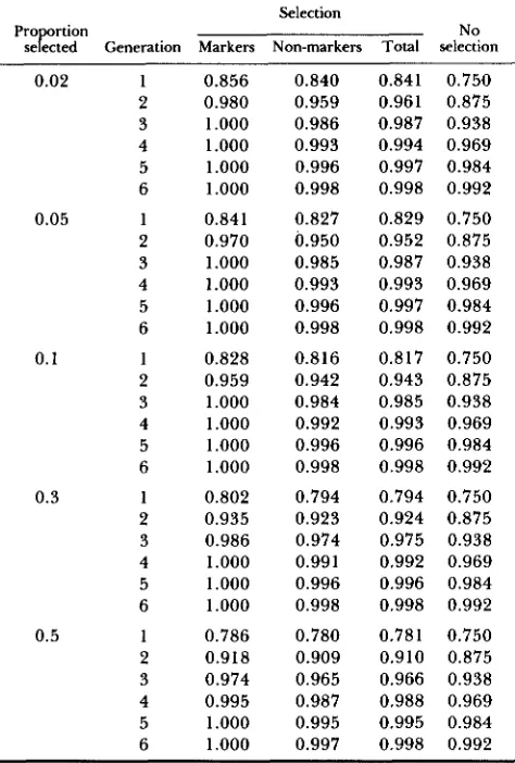
Twenty non-carrier chromosomes with two selected marker loci o n each. Selection: simulation results, mean G values after selection averaged over either marker loci only (Markers), or non-marker

loci only (Non-markers), or whole genome (Total). No selection:

Equation 1, expected G values without selection for comparison.

mated measure G was determined by simulations.

Each chromosome was 100 cM long and selection was

applied at two marker loci per chromosome, located at 20 cM from the distal telomeric loci. These locations had been previously found to be most efficient (results not shown). Table 1 shows the results obtained under continuous selection for six generations, for five values of s (2, 5 , 10, 20 and 50%). Results concerning the marker loci (third column) show that fixation occurs very rapidly at high selection intensity, markers becoming useless after fixation. T h e fourth column shows that response at non-selected loci is lower. This is illustrated in Figure 1 , showing the mean distribution of G at each locus along a chromosome.

T h e effect of increasing the number of selected marker loci is shown in Figure 2, where mean G values are given for six generations under continuous selection, with up to ten marker loci per 100 cM. T h e loci

G

0. O 4

0.8 I g 1

O.'% i o

io

i o 40 8 60 i o rio

do

l b o

I ch--(cw I

Marker Marker

FIGURE 1 .-Local response to selection along a non-carrier chro-

mosome. Data of Table 1 plotted along a virtual chromosome. Each

point corresponds to the average response over the 20 non-carrier

chromosomes at the same locations. Generations 1 to 6 of continu-

ous selection from bottom to top, with N = 200 and s = 0.1.

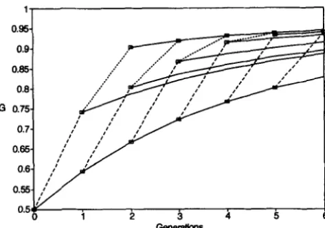
FIGURE 2.-Effect of number and localization of selected marker

loci. Twenty non-carrier chromosomes with N = 200 and s = 0.1,

generation 1 to 6 from bottom to top. Solid lines: markers evenly

spaced on each chromosome: dashed lines: equal number of markers

assigned to each chromosome, with position random; dotted lines: marker positions completely random on the whole genome.

were either evenly spaced along a known genetic map, or randomly located on each chromosome, or randomly located on the whole genome. We find that increasing the number of selected markers above three per 100 cM has poor efficiency in early generations. In later generations higher densities are relatively more efficient, but all G values are already close to 1. In practice then, two markers per 100 cM should be sufficient to get the highest possible response in the early generations if the markers are localized. Using markers with unknown chromosomal location is less useful. It was found that these results were not affected by increasing the number of chromosomes up to 30 pairs, or the population size up to 1000 (data not shown).

(4)

1202 F. Hospital, C. Chevalet and P. Mulsant

TABLE 2

Effect of different proportion s e l e c t e d in the first two

generations on mean G values after the second generation

Proportion selected in second generation Pro rtion selected

in g s t generation 1.00 0.30 0.10 0.05 0.02

1

.oo

0.875 0.897 0.910 0.914 0.920

0.30 0.909 0.924 0.932 0.936 0.941

0.10 0.925 0.936 0.945 0.947 0.951

0.05 0.933 0.942 0.949 0.951 0.956

0.02 0.941 0.949 0.955 0.957 0.961

Simulation results with twenty non-carrier chromosomes.

the first two generations only is considered in Table 2. Results are in qualitative accordance with the tendency suggested by the analytical approach for independent loci, which showed that a single selection step is more efficient the later it is applied.

Selection involving only the chromosome carry- ing the introgressed gene: In this section the genetic system involves a single chromosome, and the gene to be introgressed is located at its center. T h e chromosome length investigated is 100 cM as in the previous analyses. One marker locus on each side of the introgressed gene is considered, at a distance d from it (selection schemes with more than two markers on the chromosome are considered in the DISCUSSION). Re- sponse to selection on the carrier chromosome is lower than on non-carriers. This is due to the existence of a segment of donor genome carried along with the introgressed gene. Here, the use of selection is mostly devoted to the reduction of this segment, so that markers position ( d ) becomes a critical parameter.

The results of calculations (APPENDIX B, and appli-

cation in APPENDIX

c )

on the interaction between the

proportion selected s and the recombination rate r that corresponds to distance d during the first generation are shown in Figure 3. Each curve refers to a given value of s, and shows the expected value of G on the carrier chromosome as a function of r. For small proportions s of selected individuals, there are two local optima at rl and r2 given by

r:

+

2rl(l

-

r l ) = s and

r; = s.

For r equal to or slightly larger than r l , selection allows all single recombinant genotypes to be retained, and results in a mean G value nearly equal to 0.75.

Using more distal markers (rl

<

7

<

rp), an increased

average response is obtained which is maximal for r = r2, when only double recombinants are selected. For larger values of r , the response decreases following Equation C-1 (APPENDIX c). Double recombinants for markers at r = r2 have a larger G value than single recombinants for more proximal markers at r = r l , SO

0 . 7 5 4 4

0.65-

0.6-

0.551

0.5 0.09 0.16 0.22 0.28 (

0: 1 0:2 0.3 0.4

P m o f m r k e f f i

P (0 5 (d)

FIGURE 3.-Effect of proportion selected and marker positions

on response at carrier chromosome. Numerical solution of equa-

tions in APPENDICES B and C. Each curve shows expected G values

after one generation of selection, for a given value of proportion

selected (between parentheses). One pair of selected markers sur-

rounding the introgressed gene. r , recombination fraction between the introgressed gene and each marker; d , corresponding distance in Morgans. See text for explanations.

‘ I I

0.54

I

0 0.1 02.2 0.3 0.4 0.5

Podtbn of merkeffi (dl

FIGURE 4,”Same as Figure 3 for proportion selected s = 0.10

and 6 generations of continuous selection (from bottom to top).

Sirnulation results.

that using two markers at r = r2 would be an optimal

solution in the first generation. But in this case, the markers reach fixation after the first generation and become useless for selection in the subsequent generations, whereas choosing markers at r = rl would allow the same process to take place in the second generation (selection of single recombinants for the second marker), eventually resulting in a higher G . Such schemes with continuous selection were studied by means of simulations (see below). For larger proportions s of individuals selected the point r = r2 = s’ no longer exists. Moreover, with large values of s the response becomes a decreasing function of r as soon as r

>

r l , so that the optimum moves to r l .

(5)

TABLE 3

0.954

G

Generations

FIGURE 5.-Effect of the time when selection is applied on re-

sponse at carrier chromosome (s = 0.1, d = 10 cM). Analytical and

simulation ( N = 200) results. Solid lines: evolution without selection;

dashed lines: first generation of selection; dotted lines: second

generation of selection. Squares indicate possible shift between selection and no selection.

tions. As recombination events accumulate over time, the apparent recombination rate between a marker and the introgressed gene increases, so that optimal values for r are smaller when later generations are considered. Figure 4 clearly shows that the choice of the markers depends on the number of generations during which selection is to be performed. Markers close to the introgressed gene are useful in later generations only (for this intermediate value of S) whereas more distal markers should be used in the short term.

The effect of the time when a single selection step is applied is illustrated in Figure 5. These results were obtained by numerical solution of the equations in APPENDIX B, and fit the simulation results well. In most cases with two markers a single selection step is more efficient if applied later as shown by Figure 5.

This tendency is in accordance with that found previously for selection on non-carrier chromosomes. Note however that exceptions to this rule can be found when markers are far from the introgressed gene (results not shown).

Applying selection more than once was investigated by simulation. Results of two successive selection steps are included in Figure 5. T h e case of continuous selection is not shown, but appeared to be equivalent to selecting only during the first t w o generations. Hence, in this example ( N = 200, d = 10 cM, s = 0.10), it turns out that fixation of both markers occurs within two generations of selection regardless of when selection is performed (cases with two non- successive selection steps give the same outcome).

Selection on the whole genome: Table 3 presents results of simulations similar to those presented in Table 1 , but with one of the 20 pairs of chromosomes bearing the introgressed gene at its center. T h e mean

Continuous selection on both carrier and non-carrier

chromosomes

Carrier chromosome Generation Selection No selection

1 0.636 0.607

2 0.747 0.684

3 0.855 0.74 1

4 0.891 0.784

5 0.903 0.817

6 0.9 13 0.842

Non-carrier chromosome Selection No selection

0.817 0.750

0.943 0.875

0.983 0.938

0.993 0.969

0.996 0.984

0.998 0.992

Same as Table 1 with one carrier and nineteen non-carrier

chromosomes. Simulation results, proportion selected 3 = 0.10.

Proportbnseleded

FIGURE 6.--Selection on the whole genome. G values after selec-

tion on carrier chromosome (dotted line) and residual intensity i

for selection on non carriers (solid line) for different proportions

selected. Analytical results for one generation of selection with d =

20 cM.

response over the whole genome is only slightly lower than with no introgressed gene, but the results high- light the large difference between the chromosome carrying the gene and the other chromosomes. When using an index with equal weights, selection on the markers has poor efficiency for the carrier chromosome.

If markers are available near the introgressed gene as well as on other chromosomes it is possible to combine selection on all these markers. In the first generation an analytical analysis is possible (APPENDIX

c)

under the approximation whereby the whole genome is described by independent loci. Figure 6 shows the joint pattern of expected G values after selection on the carrier chromosome, and of the remaining intensity i of selection that can be exerted on the other chromosomes. Assuming that the first priority of selection is to reduce the length of the donor segment surrounding the introgressed gene, individuals selected in this first step of selection may then be screened according to their G value for the rest of the

genome, provided they are more numerous than

(6)

Generation 1

10.79

Generation 2

Generation 3

Generation 5

Generation 4 0 . q

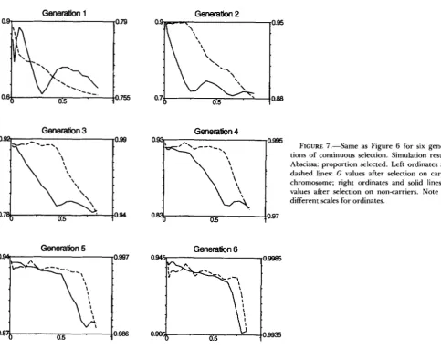
FIGURE 7.-Same as Figure 6 for six genera-

tions of continuous selection. Simulation results. Abscissa: proportion selected. Left ordinates and dashed lines: G values after selection on carrier chromosome; right ordinates and solid lines: G

values after selection on non-carriers. Note the different scales for ordinates.

0.

0.5 0.97

Generation 6

0.9985

, ,09935

recombinant individuals for the carrier chromosome are not numerous enough, the additional (non-recombinant) individuals needed may be chosen according to their overall recipient genome content. Finally, if the number of recombinants for the carrier chromosome is equal to the number of individuals needed to reproduce the population, other chromosomes are

chosen at random as far as their recipient genome content is concerned. Hence, the combinations (s,

q )

and (s, r2) of parameters that were found optimal in the preceding section when only the carrier chromosome was considered, are the worst for the non-carrier chromosomes when the whole genome is considered. T h e results of simulations for several generations of continuous combined selection are shown in Figure

7

for both carrier and non-carrier chromosomes. The points with reduced response move to larger values of

s as later generations are considered, so that the situation in later generations may seem less dramatic than the one described above for the first generation. Note however that the values of G for non-carrier chromosomes must be compared to the corresponding values with no selection (0.75, 0.875,

. .

.).

DISCUSSION

Efficiency of markers for overall recipient ge- nome recovery: From a quantitative and practical point of view the predicted gain in time expected from marker selection is about two backcross generations. If the proportion selected is less than ten percent, the recipient genome content after selection in the third generation is equal to or larger than that expected without selection at the fifth generation. Although significant, these predictions are less opti- mistic than those given by HILLEL et al. (1990). Ac- cording to our results (Table l ) , two generations of continuous selection are needed to get a response equal to their predictions for a single selection step (Table 3 with 40 segments, in HILLEL et al. 1990). Also, their calculations for continuous selection (Table 5, HILLEL et al. 1990) predict quasi-fixation within two generations, a result at variance with ours (Table

(7)

were independent loci, so that their results are com- parable only to our restricted approach developed in

APPENDIX A. T h e difference stems from the effects of

recombination between the selected marker loci and the surrounding loci (Figure 1). A practical and im- portant consequence of these discrepancies is that we find that stopping selection after the second backcross generation is not a correct strategy. As shown in Table 1, substantial gains from selection are still expected at the third generation for any selection intensity, and all the more as selection is less intense. This trend is in accordance with the qualitative analytical result of

APPENDIX A. Therefore, if marker assisted introgres-

sion is to be applied, it should be performed during at least three generations. Moreover, if only low selection intensity (s

>

0. IO) can be applied, selection should proceed longer in order to achieve a savings of about two generations over a six generation interval.

Using markers to monitor gene introgression was found to be most useful if linkage maps are available. A proper choice of evenly spaced markers allows a minimal number of them to be used. If only markers of unknown chromosomal location are used, as would be the case with VNTRs, the response is reduced (Figure 2). T h e increased efficiency due to mapped markers may not seem worth the work needed to establish the genetic map. However, one should note that the additional gain due to mapped markers may represent up to '/9 of the advance due to selection with

non-mapped markers. Furthermore, with non-

mapped markers one takes the risk that some chromosomes are under no control. This risk is eliminated if every chromosome can be marked by randomly located syntenic loci (provided for example by probes from chromosome specific libraries). In this latter case the response is only slightly lower than with evenly spread markers.

A density of two to three markers per 100 cM seems to be an optimal choice, since increasing this density is of small benefit. This result may seem somewhat surprising, and contrary to current opinion. It can be explained by considering the distribution of donor genes in the genome. In early generations, few recombination events have occurred, so that donor genes should be represented by a few long segments on each chromosome. Since one selected marker by segment is enough to control it, only a few markers per chromosome are needed. As recombination events accumulate over time, the number of donor segments spread over the genome increases, and their length decreases, so that more and more markers are needed to control all of them. A higher density of markers might then be useful in later generations to eliminate these donor segments more rapidly. Indeed, this seems to be the case since in later generations the use

of many markers appeared to be relatively more efficient than using only a few (results not shown). But practical gains are very low since all G values are then over 0.99. Hence, increasing the number of markers does not seem efficient under the special conditions of gene introgression. Investigating this efficiency in a more general framework of marker assisted selection would require further analyses, not restricted to average genome content, but also devoted to the distribution of segment lengths (STAM and ZEVEN (1 98 1).

Use of markers surrounding the introgressed gene: Our analysis has focused on the simple case where a single pair of markers controlling the introgressed gene is used in the selection scheme. Knowing the intensity of selection that can be applied, it pro- vides a basis for choosing such a pair when several markers are available on the carrier chromosome. The interesting result is the potential use of rather distal markers during the first generations, which may pro- vide a significant recovery of the recipient genome, even if the length of the donor segment carrying the introgressed gene is not reduced to the minimum in this process. Indeed, if proximal markers are also available, it is not harmful to wait until later generations to select for them, since the efficiency of selection generally increases with time. Furthermore, selecting only for very proximal markers is clearly inef- fective if the population size is not very large.

Hence, we suggest using a more complex strategy of selection to make the most of all the markers available on the carrier chromosome. This strategy is suggested by the results presented in this paper concerning the classical case of a single pair of markers controlling the introgressed gene. It consists of giving preference to the selection of proximal recombinants as soon as they arise, but not ignoring more distal recombinations. In practice, this would be easy to do when typing the individuals. Some theoretical results that give an idea of the efficiency of such a strategy are presented in Table

4.

They were obtained by using a selection index such that the weight of a proximal single recombinant is larger than the sum of weights of all more distal double recombinants. Table

(8)

TABLE 4

Use of several markers surrounding the introgressed gene

Population

Selection on single pair

Multi-marker size Generation 1 cM 2 cM 5 cM 10 cM selection

20 3 0.793 0.834 0.901 0.905 0.918

6 0.912 0.947 0.953 0.940 0.977

50 3 0.820 0.873 0.916 0.914 0.928

6 0.942 0.964 0.955 0.939 0.982

100 3 0.861 0.898 0.933 0.917 0.937

6 0.970 0.968 0.959 0.938 0.981

200 3 0.865 0.912 0.927 0.918 0.942

6 0.975 0.968 0.955 0.943 0.981

Four pairs of markers are located at 1 , 2, 5 and 10 cM on each

side of the introgressed gene. G values after selection performed

on an index combining the four pairs of markers (last column), as

explained in the text, can be compared to G values after selection

performed on only one of the four pairs. Simulation results, pro-

portion selected s = 0.10.

for a few very proximal markers. Moreover, reducing the number of individuals may accelerate the experi- ment and reduce its cost, especially for animal species. Whereas a significant improvement in recipient genome recovery is expected with the use of markers linked to the introgressed gene, as compared to the expectations under no selection (STAM and ZEVEN

1981), it is worth stressing that when the proportion selected exceeds ten percent it does not seem possible to get a process of introgression on the carrier chromosome that is faster than the random process on non-carrier chromosomes. This is probably due to the short time interval considered. T h e first aim of selection on the carrier chromosome is to sort out recombinants near the introgressed gene. Once this is achieved the carrier chromosome, except for the segment surrounding the gene, behaves like the non- carrier chromosomes and can be submitted to selection. However, most of the markers selected during the initial step will have reached fixation, and then introgression will proceed as if without selection, unless other polymorphic markers can still be found on the chromosome.

Selection on the whole genome: Two subsets can be distinguished in the total foreign genome present in a gamete from a crossed parent. T h e first is the continuous segment surrounding the introgressed gene on the carrier chromosome, and the second is the other segments spread on non-carrier chromosomes or on telomeric parts of the carrier chromosome. The efficiency of selection is not the same for these two subsets. Since, by definition, any individual candidate for selection is carrying the introgressed gene, the foreign genome around this gene is strongly retained, and selection is less efficient. Moreover, the results show that it does not seem possible to simulta- neously optimize selection for both the carrier and

non-carrier chromosomes. Hence, a decision must be taken as to the efficiency of selection for each part of the genome.

Selection could be performed using an index on the markers of all chromosomes, according to the princi- ple described in the previous section. For example, in order to attain equal efficiencies of selection for the two subsets of foreign genome, the relative weight in the index of the markers devoted to the control of the foreign segment surrounding the introgressed

gene should be equal to the proportion of the total foreign genome due to this segment. This value will depend on the genome size and the generation considered. Some examples are shown in Table 5. Such an index could be further refined to take into account qualitative considerations concerning the distance between recipient and donor genomes (for example, if the donor is a wild species, priority might be given to eliminating detrimental genes on non-carrier chromosomes), or the presence of favourable genes near the introgressed one that should be kept with it on the carrier chromosome.

CONCLUSION

Our results show that markers are useful in gene introgression programs. T h e selection strategy to be applied should take into account the available material and conditions, and should determine when and how strongly to select, and which markers to use. A com- mon approach is to select as early as possible, and as strongly as possible on markers very close to the introgressed gene, generally without paying much

attention to non-carrier chromosomes. We have

shown that this is not always the best strategy. Three of our results might be kept in mind when seeking an optimal selection strategy in gene introgression programs:

First, for the carrier chromosome, the response to selection is a function of both the distance between the markers and the introgressed gene, and the proportion of selected individuals.

Second, once a first step of selection has been performed on the carrier chromosome, it is still possible to select on non-carrier chromosomes, although the intensity of selection available for the latter depends on that applied to the former.

Third, the later the selection is performed, the more efficient it is. We showed this point both analyt- ically (for a single generation of selection) and by simulation (for several generations of continuous selection).

(9)

Marked Assisted Gene Introgression

TABLE 5

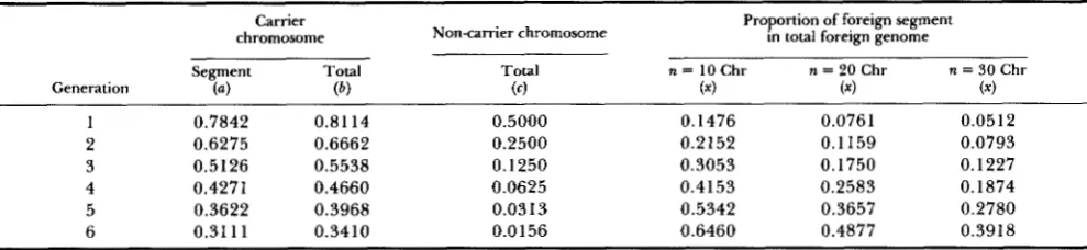
Distribution of foreign genome without selection on a gamete from a crossed parent

chromosome Carrier

Non-carrier chromosome

Total

Proportion of foreign segment in total foreign genome

n = 10 Chr n = 20 Chr n = 30 Chr Generation

Segment Total

( 4 (6) (4 ( 4 ( 4 ( 4

1 0.7842 0.8114 0.5000 0.1476 0.0761 0.051 2

2 0.6275 0.6662 0.2500 0.2 152 0.1159 0.0793

3 0.5 126 0.5538 0.1250 0.3053 0.1750 0.1227

4 0.4271 0.4660 0.0625 0.4153 0.2583 0.1874

5 0.3622 0.3968 0.031 3 0.5342 0.3657 0.2780

6 0.31 1 1 0.34 10 0.0156 0.6460 0.4877 0.3918

( a ) length of foreign segment surrounding the introgressed gene relative to carrier chromosome length; ( b ) proportion of foreign genome on carrier chromosome; (c) proportion of foreign genome on non-carrier chromosomes; (x) proportion of (a) relative to the overall foreign genome of the gamete. x = a / [ b

+

( n

-

l)c] where n is the number of chromosomes.

Hence, for intermediate selection intensity, a better strategy is either to select in the short term for markers further from the gene, or to wait for a few generations until recombinants for markers close to the gene can accumulate in the population. This choice will depend on the genetic map available for the species selected. Of course, if many markers are available, selection could be performed both in the short term for markers far from the gene, and later for markers closer to it. Whereas the general belief is that one need pay attention only to markers close to the introgressed gene, our results emphasize the impor- tance of distant markers in most cases.

Thanks are due to F R A N ~ I S RODOLPHE, ALAIN CHARCOSSET,

ISABELLE OLIVIERI, DANIEL WALLACH and NIGEL GRIMSLEY for

careful reading of the manuscript.

LITERATURE CITED

FISHER, R. A , , 1949 The Theory of Inbreeding. Oliver & Boyd,

Edinburgh.

HANSON, W. D., 1959 Early generation analysis of lengths of

heterozygous chromosome segments around a locus held heterozygous with backcrossing or selfing. Genetics 44: 833-837.

HILLEL, J . , T. SCHAAP, A. HABERFELD, A. J. JEFFREYS, Y. PLOTZKY,

A . CAHANER and U . LAVI, 1990 DNA fingerprint applied to

gene introgression breeding programs. Genetics 1 2 4 783-789.

LANDE, R., and R. THOMPSON, 1990 Efficiency of marker-assisted

selection in the improvement of quantitative traits. Genetics

124 743-756.

STAM, P., and A. C. ZEVEN, 1981 The theoretical proportion of

the donor genome in near-isogenic lines of self-fertilizers bred by backcrossing. Euphytica 30: 227-238.

YOUNG, N. D., and S. D. TANKSLEY, 1989 RFLP analysis of the

size of chromosomal segments retained around the Tm-2 locus

of tomato during backcross breeding. Theor. Appl. Genet. 77:

353-359.

Communicating editor: B. S. WEIR

APPENDIX A

Response to selection at L independent loci: We consider a set of L independent marker loci where

alleles from the donor and recipient lines can be distinguished, and assume that selection is performed in a population of infinite size. T h e trait selected for is the frequency G of recipient alleles at the marker loci. If selection is applied at generation (g), the expected response to selection depends on the proportion of selected individuals, and on the variance of G among zygotes of the gth generation.

In a gth generation backcrossed individual, let X( g) be the number of recipient alleles received from its crossed parent. The proportion of recipient alleles is then

G(g) = [ L

+

X(g)I/(2L) = 1/2

+

(1/2)(X(g)/L).

E[X(g)ll

Var[X(g

+

l)] =

(94)

( L

-

E[X(g)])

+

(%)Var[X(g)]

using initial conditions in F1 that X(0) = 0, Var[X(O)] = 0 we then have

E [ X ( g ) ] = L[1

-

('/2)9 Var[X(g)] = L [ ( Y i ) g

-

(94)gI. Without selection we thus have

E[G(g)] = 1

-

(1/2)@1

(10)

1208 F. Hospital, C. Chevalet and P. Mulsant

Now we consider that selection is applied for the first time during the gth generation, with a proportion (s) of selected individuals. If L is large enough, the distribution of G is nearly Gaussian, and the expected advance due to selection can be approximated by

Int(s).(Var[G(g)])'"

where Int(s) is the expectation of the truncated reduced normal distribution with tail frequency (s). After selection the expected frequency of recipient marker alleles is then approximately equal to

If no selection is applied during the next generations, the expected proportion follows the usual recurrence relation

E [ G ( k

+

l)] = (l/z)E[G(k)]

+

(Yz) for k L g. T h e overall result after n generations, involving only selection during the gth generation is thus approximately equal to:

This expression is maximal if (g) is maximal, that is, the highest response is obtained if selection is performed during the last generation.

APPENDIX B

Response around the introgressed gene: A similar analysis can be done on the chromosome carrying the introgressed gene, although the analysis is compli- cated by taking account of recombinations. Following

HANSON (1959) and STAM and ZEVEN (1981), we assume that the number of crossing overs along a chromosomal segment of length ( u ) Morgans follows

a Poisson law with mean ( u ) , and we compute the frequency of the recipient genome at any locus (x) on the chromosome. (Strictly speaking, we consider probability densities.) We consider one half of the chromosome, from the locus of the introgressed gene (locus 0) to one telomere (locus at distance

I,

the length of the half chromosome), and on this half chromosome a marker locus at distance d from the introgressed gene. Let x(u,g) be the frequency of recipient alleles

at locus u , generation g.

Densities of recipient alleles in offspring: Without taking account of the marker locus, the proportion of recipient alleles at locus u in the next generation can

be written as

x(u,g

+

1) = T ( u ) * 1

+

(1

-

+

1) =

r ( d ) * X ( U ? g)

for 0

<

u

<

d. From the marker to the telomere, we get a relation similar to that given in Equation B1:

<

u

<

1.

(b) T h e case of no recombination (the offspring carries a donor allele at the marker locus), occurs with probability [ l - r(d)]. In this case, the probability of recombination between the introgressed gene and a locus ( u ) , 0

<

u

<

d , is equal to the probability that recombinations occur in both segments IO, u [ and ]u, d [. T h e total probability of no recombination between 0 and d is then split into two terms: 1

-

r ( d )

(11)

Marked Assisted Gene Introgression

x(u,g

+

1) = [ l

-

r(u)].[l

-

r(d

-

u)]

1

-

r ( d ) * X(U&

for 0

<

u < d. From the marker to the telomere we then have the same relationship as in Equation B1 without selection:

From the beginning of the process to the time of recombination, densities change according to Equa- tions B4 and B5; at the time of recombination, densities are given by Equations B2 and B3; then from the time of recombination to the time of selection, densities change following Equation B1. Since selection is applied at generation (g), the expected proportion of non recombinant individuals is

[1

-

r(d)lg

and the complementary proportion R(g) of recombinants is the sum over CY of the probabilities

r(d)-[l

-

r ( d ) r - l

that the recombination event took place between generations ( a

-

1) and

(CY),

a = 1 , 2,

.

., g. Combining

these probabilities with the evolutionary rules (B4) and (B5) before recombination, (B2) and (B3) at recombination, and then (Bl), yields t w o densities

."(u,g), and x""(U,g)

for recombinant and non recombinant individuals in generation g.

The relative proportion of recombinant to non recombinant individuals is increased in the selected population. Assuming for simplicity that the introgressed gene is in the middle of the chromosome, with two half chromosomes of length (1) and markers at distance ( d ) on each side, selecting a proportion (s) of individuals yields the following densities x*(u,g) in the selected population (R(g) is the expected proportion of recombinants on one half chromosome)

if:

s

<

R(gY

then only double recombinants are selected for, so that

x*(u,g) = xR(u,g) if:

then a mixture of double and single recombinants are kept and so

x*(u,g) = R(g)2R(u,g) S

if:

s>R(g)2+2.R(g).[I -R(g)],

all three genotypes at the marker may be kept. Then

Thereafter, from generations (g) to (n), densities change according to Equation B1, starting with their values x * obtained after selection during the gth generation.

Results were obtained numerically by calculating the preceding densities at a large number of distinct loci (1 00 and 1000 per Morgan), and summing them along the chromosome length to get mean recipient genome content G .

APPENDIX C

Combined selection in the first generation: Selec- tion aimed at reducing the length of the donor segment surrounding the introgressed gene may be combined with global selection for the recipient genome on other chromosomes, provided that the selection intensity is sufficiently great.

We assume that selection is performed during the first backcross generation. As in APPENDIX B, we as-

sume a pair of markers surrounding the gene at a distance ( d ) corresponding to a recombination fraction r = r ( d ) , on each half chromosome of length (1).

Recombinant individuals that carry the recipient allele are kept. T h e expected recipient genome content

G

is derived, both in recombinant and non recombinant offspring, from Equations B2,B3 and B4,B5, respectively. Similarly, the expected length of the donor genome segment around the gene can be calculated in both genotypes. One gets the following expressions. (Note that the mean results Of STAM and ZEVEN (1 98 1)

(12)

1210 F. Hospital, C. Chevalet and P. Mulsant

In double recombinants (proportion r 2 ) :

/p

= 2 [ 1 - exp(-d)]' 1

-

exp(- 2d) '

In single recombinants (proportion 2r( 1 - r)):

G N R =" 1 1

-

exp(-2d)

2 4.1.[ 1

+

exp(-2d)] (C2a)

/ p

= [ 1

-

exp(-d)]' 1

-

exp(-2d)

1

-

exp(-2d) 1

+

exp(-2d)

@ N N = 2 1

-

exp(-2d) exp(-d)

-

exp(-1)

1

+

exp(-2d)

+ 4