Stability Analysis of a Discrete Prey - Predator Model with Ratio Dependence

Stability Analysis of a Discrete

Prey - Predator Model with Ratio Dependence

M.Reni Sagaya Raj1,A.George Maria Selvam2 and V.Sathish3

Head & Associate Professor of Mathematics, Sacred Heart College, Tirupattur – 635 601, S.India1 Associate Professor of Mathematics, Sacred Heart College, Tirupattur – 635 601, S.India2 M.Phil Scholar, Dept.of Mathematics, Sacred Heart College, Tirupattur – 635 601, S.India3.

Abstract: In this paper, a discrete food web system with ratio-dependent functional response is proposed and analysed. The model is characterized by a coupled system of first order non-linear difference equations. The fixed points are computed and criteria for stability of the system are obtained. Time plots and the phase portraits are obtained for different sets of parameter values. The numerical simulations not only illustrate the validity of our results, but also exhibit more complex dynamical behaviours.

2010 Mathematics Subject Classification. 39A30, 92D25.

Keywords and phrases: difference equations, predator – prey system, fixed points, stability.

I. INTRODUCTION

Biological interactions are the relationships between two species in an ecosystem in ecology. Predator–prey interaction has always been an important issue in mathematical modelling of ecological processes. The dynamical relationship between predators and their prey is one of the dominant themes in ecology. Alfred John Lotka (1880-1949) and Vito Volterra (1860-1946), the most prominent founders of mathematical ecology, investigated the dynamics of interacting populations [3]. Considerable progress has been made since the famous Lotka–Volterra predator–prey models. An important form of predator-dependent functional response is the ratio-dependent response. Predator-prey models with such ratio-dependent functional response are strongly supported by numerous field and laboratory experiments [4].

II. MODEL DESCRIPTION AND FIXED POINTS

This paper presents a model which attempts to represent the population dynamics which can occur in a system when two species interact with each other in the same environment. There are examples of populations which are easy and appropriate to describe by discrete times models. Discrete time models are easy to formulate and to simulate [1,2,5,6,7]. In this paper, the dynamics of a ratio-dependent discrete predator-prey system with the logistic growth in prey and the functional response is discussed. The conditions for the existence and local stability of the system are obtained. We consider the following system of difference equations which describes interactions between two species with functional response.

where r, a, c, d





 

  

 

   

_{ }



 

  

   

_{ }

 

2

1 1

1 1 ... 1

a x n y n

x n r x n rx n

b x n d x n y n

y n c y n

b x n

    



   

 













0 1 2 2

1 0, 0 , 1, 0 bc , rbd d c b

E E and E

c d _{a c d}

  _   _     _{ }  _  

provided c d 0 andb d c.

c



  

III. ANALYSIS OF FIXED POINTS

The qualitative analysis of nonlinear dynamical systems has become increasingly widespread and has been used in theoretical ecology. One of the most useful techniques for analysing nonlinear systems qualitatively is the analysis of the behaviour of the solutions near fixed points using linearization. The local stability analysis of the model can be carried out by computing the Jacobian corresponding to each fixed point. The Jacobian matrix J for the system (1) is









 

( , ) ... 2

1

aby ax

r rx

b x

b x

J x y

bdy dx c b x b x  _{   }   _{ }                

whenE₀(0, 0), the Jocobian matrix (2) becomes 0

1 0 ( ) 0 1 r J E c      _    ,

The Eigen values are ₁ 1 r,₂  1 c.

Proposition: 1

The equilibrium point E₀ is

(1) Sink if 2  r 0 and 0 c 2. (2) Source if r0andc2. (3) Saddle if r0 andc2.

(4) Non hyperbolic if either r0 or c2.

whenE₁(1, 0), the Jocobian matrix (2) becomes ₁ 1 1 ( ) 0 1 1 a r b J E d c b  _{ }   _      _{ }   _    ,

The Eigen values are ₁ 1 , ₂ 1 . 1 d r c b         Proposition: 2

The equilibrium point E₁ is

(1) Sink if 0 r 2 anddc b





(2) Source if r2 anddc b





(3) Saddle if r2 and dc b





(4) Non hyperbolic if either r2 ordc b





when









2 2

1

, rbd d c b

bc E

c d a c d

The Jocobian matrix (2) becomes









2

( ) 1

( )

1

1

rbc c d rc ac

d c d d d

J E

r d c b a



 _{  } 

 _ 

 



 _{   } 

 

 

,

 





_

_



 





_

_

( 1) ( 1)

( ) ( )

2 rc rbc c d , 1 rc d c b rbc c d .

B Tr J E C Det J E

d d c d d d c d

   

 _ 

       

 

Proposition: 3

The equilibrium point E₂ is (1) Sink if A₁ b A₂.

(2) Source if bA₁andbA₂.

(3) Saddle if bA₁.

(4) Non hyperbolic if either bA₁orbA₂.

where

















1 2

( ) ( 2) 4 ( ) ( ) 1

, .

2( ) ( ) (1 ) (1 )

c d rc c d d c d c d

A A

rc c d c c d c c d c

      

 

     

IV. NUMERICAL SIMULATIONS

In this section, we illustrate the analytical findings with the help of numerical simulations performed with MATLAB. We present time-plots and phase portraits for system (1) to confirm the theoretical results with hypothetical set of data. They show interesting complex dynamical behaviours.

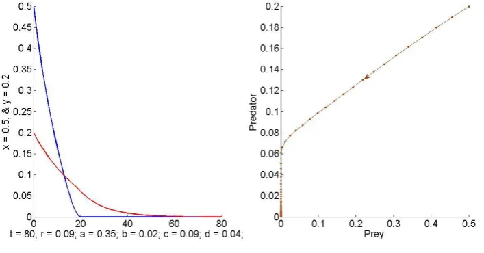
Example 2. Considerthe values r = 0.09, a = 0.35, b=1.24, c = 0.09 and d = 0.04. For this choice of parameter values the unique axial equilibrium point E1 = (1, 0) is stable. Eigen values are 1 = 0.91 and 2 = 0.93 so that 1,2 < 1.

Hence the equilibrium point is stable. The time plot and the phase diagram illustrate the result and predator is extinction, see Figure - 2.

Figure - 2.

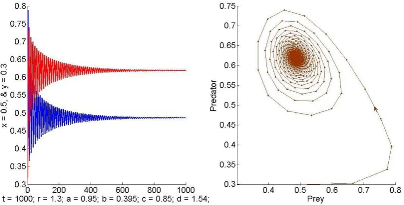
Example 3. In this example, we take r = 1.3, a = 0.95, b = 0.395, c = 0.85 and d = 1.54. Computations yield E2 = (0.48, 0.62) which is a point in the first quadrant of 2

.

 The Eigen values are _1,2 = 0.8679± i0.4866 and _1,2 = 0.9950 < 1. Hence the criteria for stability are satisfied. Evidently both species converge to equilibrium. The phase portrait in Figure - 3 shows a sink and the trajectory spirals towards the equilibrium point E2.

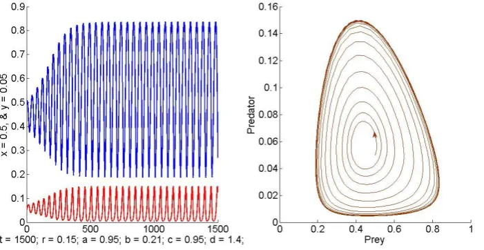
Example 4. When we take r = 0.15, a = 0.95, b = 0.21, c = 0.95 and d = 1.4, the phase portrait in Figure – 4 shows the existence of a limit cycle.

Figure - 4.

V. CONCLUSION

The classical Lotka-Volterra model of predicts cyclical behaviour of predator – prey populations and this model is rich in dynamics but unrealistic in nature. This paper dealt with a realistic description of interacting populations with the introduction of a functional response. Fixed points are computed and the behaviour of the solutions near fixed points is determined by the Jacobian matrix of the system. Stability conditions are established and phase plane analysis is carried out by numerical simulation with hypothetical sets of parameters which exhibits rich dynamics of discrete model.

REFERENCES

[1] Agiza, H. N.,Elabbasy, E. EL- Metwally, M. H., & Elasdany, A. A. “Chaotic dynamics of a discrete prey-predator model with Holling type II”. Nonlinear Analysis: Real World Applications, 10, 116-129, 2009.

[2] Danca, M.,Codreanu, S. & Bako, B. “Detailed analysis of a nonlinear prey-predator model”. J. Biol. Phys., 23, 11-20, 1997. [3] Leah Edelstein-Keshet, “Mathematical Models in Biology”, SIAM, Random House, New York, 2005.

[4] Meng Fan and Qian Wang, “Dynamics of a non-autonomous ratio-dependent predator-prey system”, Proceedings of the Royal Society of Edinburgh, 133A, 97-118, 2003.

[5] M.Reni Sagaya Raj, A.George Maria Selvam, R.Janagaraj, “Stability in a Discrete Model of Prey-Predator Interactions”, International Journal of Latest Research in Science and Technology, ISSN (Online):2278-5299, Volume 2, Issue 1: Page No.482-485, January-February 2013. [6] M.Reni Sagaya Raj, A.George Maria Selvam, R.Janagaraj and D.Pushparajan, “Dynamical Behavior in a Discrete Prey-Predator Interactions”,