Thiemichen, Stephanie (2016): Extensions of exponential random graph models for network data analysis. Dissertation, LMU München: Fakultät für Mathematik, Informatik und Statistik

(1)

Stephanie Thiemichen

Extensions of Exponential Random

Graph Models for Network Data

Analysis

Dissertation an der Fakultät für Mathematik, Informatik und Statistik der Ludwig-Maximilians-Universität München

(2)

(3)

Stephanie Thiemichen

Extensions of Exponential Random

Graph Models for Network Data

Analysis

Dissertation an der Fakultät für Mathematik, Informatik und Statistik

der Ludwig-Maximilians-Universität München

(4)

Erster Berichterstatter: Prof. Dr. Göran Kauermann

Zweiter Berichterstatter: Prof. Dr. Ernst Wit

(5)

Danksagung

(6)

(7)

Danksagung

Mein besonderer Dank gilt allen, die zur Entstehung dieser Doktorarbeit in der ein oder anderen Form beigetragen haben. Das sind . . .

. . . mein Doktorvater Göran Kauermann. Vielen Dank für die Betreuung und das gemein-same Durchstehen aller Probleme, die sich beim Einarbeiten in ein komplett neues Gebiet gerade am Anfang (und danach auch immer wieder) ergeben. Danke auch für den Kontakt-aufbau zu einigen der Koriphäen im Bereich der statistischen Netzwerkanalyse. Networking ist eben wichtig.

. . . my co-authors Alberto Caimo and Nial Friel. Thanks for the great time in Dublin, all the fruitful discussions, the code debugging, the help with the paper revisions, and especially the insights into Bayesian methods.

. . . Ernst Wit for the great workshop in Leiden on Statistical Network Science, and for agreeing to take the job as external examiner.

. . . meine langjährige Bürokollegin Linda Schulze Waltrup. Danke fürs Zuhören, wenn nötig in Ruhe lassen, fürs Pflanzen pflegen und fürs Sofa retten.

. . . meine Kollegen Verena Maier, Ludwig Bothmann und Michael Windmann. Danke für die entspannte Atmosphäre am Lehrstuhl, das Zuhören und das ab und zu Vorbeischauen, damit ich nicht vereinsame.

. . . Julia Kopf, Tina Feilke und Bernd Budich. Danke für die Hilfe beim Korrekturlesen der Arbeit, dass ihr mich zwischendurch immer wieder aufgebaut habt und vor allem danke für die langjährige Freundschaft.

. . . alle am Institut. Es herrscht wirklich eine unglaublich angenehme familiäre Atmosphäre, ohne die sowohl Studium, als auch Dissertation nur halb so schön gewesen wären. Danke dafür!

. . . meine Familie und Freunde, allen voran meine Eltern Karin Leon und Berthold Thiemichen. Danke, dass ihr mich immer unterstützt und dabei nicht zu oft nachgefragt habt, wie es denn so läuft.

(8)

(9)

Zusammenfassung

Die Analyse von Netzwerkdaten gewinnt als Gebiet in der Statistik zunehmend an Bedeutung. Dabei sind sowohl die Modellierung selbst, als auch die damit verbundenen computationalen Aspekte herausfordernd. Sogenannte Exponential Random Graph Mo-delle (ERGM) sind ein bekannter und häufig genutzter Modellierungsansatz für solche Daten.

Diese Arbeit gibt zunächst eine kurze generelle Einführung in Exponential Random Graph Modelle zur statistischen Netzwerkanalyse. Vorteile und Probleme dieser Modellklasse wer-den diskutiert, wobei speziell das Problem der Modelldegeneriertheit beleuchtet wird. Die Dissertation beinhaltet zwei Beiträge zur Erweiterung von Exponential Random Graph Modellen. Die erste Erweiterung beruht auf einem Bayesianischen Ansatz. Dabei soll es ermöglicht werden, knoten-spezifische zufällige Effekte ins Modell aufzunehmen, um Heterogenität in den Knoten zu kompensieren. Der Ansatz basiert auf den von Caimo und Friel (2011) entwickelten Methoden für Bayesianische Exponential Random Graph Modelle. Zusätzlich zur Prozedur für die Modellanpassung wird eine approximative, aber praktikable Berechnung für Bayesfaktoren zur Modellselektion entwickelt. Die zweite Erweiterung nutzt einen Stichprobenansatz basierend auf der konditionalen Unabhängigkeitsstruktur eines Netzwerkes (wenn Markov-Unabhängigkeit angenommen wird) und erlaubt es große Netzwerke mit mehr als 1000 Knoten zu analysieren. Nicht-lineare Statistiken in Kombi-nation mit einem penalisierten Glättungsansatz werden mit ins Modell aufgenommen, um das resultierende Modell zu verbessern und zu stabilisieren.

(10)

(11)

Summary

The analysis of network data is an emerging field in statistics which is challenging both model-wise and computationally. The so-called Exponential Random Graph Model (ERGM) is one particular well-known and widely used modelling approach for such data. This thesis starts with a short general introduction to Exponential Random Graph Models for statistical network analysis. Advantages and problems of this model class are presented with a special emphasis on the issue of model degeneracy. This dissertation contains two contributions which try to extend the existing Exponential Random Graph Models. The first extension uses a Bayesian approach in order to incorporate nodal random effects into the model to compensate for heterogeneity in the nodes of a network. It is based on the methodology developed by Caimo and Friel (2011) for Bayesian Exponential Random Graph Models. In addition to the model fitting procedure, an approximate but feasible calculation of the Bayes factor for model selection is developed. The second extension is based on a subsampling approach which utilizes the conditional independence structure of a network (if Markov independence is assumed) and allows to analyse larger networks with more than a thousand nodes. Non-linear statistics are added to the model using a penalized smoothing approach in order to improve and stabilise the resulting model.

(12)

(13)

1 Introduction

“It is strange that the assumption that data obtained from human respondents represents independent replications has been so pervasive in statistical models used in sociological research.”

Tom A. B. Snijders (Snijders, 2016)

The field of network data analysis has gained more and more interest in recent years. In addition to the fact that a lot of network datasets are available, there is a wide range of possible applications, which often have been the driving forces behind method development in this field. Ranging from biological networks, such as genetic or metabolic pathways or gene regulatory networks, over technical and communication networks, to economic (e.g., company cooperations or trade flows) and – of course – social networks, the main feature of all of these data collections is its relational structure. Referring to Snijders quote at the beginning: Especially – but not only – in the sociological context, ignoring the relations and the thereby induced dependence structures among actors in an analysis may result in questionable conclusions. Dealing with relational structures and its dependencies is very challenging from a statistical point of view. Almost every basic statistics course contains the sentence “We assume the observations to be independent and identically distributed (i.i.d.).”, and the case of having observations which are not (conditionally) independent is not even considered in a lot of statistical curricula, especially if its only taught as a minor subject. The assumption of dealing with (at least conditionally) independent observations is almost always violated in the network context. This impedes, or even prevents the use of a lot of standard statistical models, as ignoring the interdependencies usually flaws the whole analysis.

Kolaczyk (2009) gives a gentle and comprehensive introduction to the field of statistical network analysis. The survey articles of Goldenberg et al. (2010), Hunter et al. (2012), Fienberg (2012), and Salter-Townshend et al. (2012), discuss recent statistical approaches, challenges, and developments in this domain.

(16)

1 Introduction

The emphasis of this thesis lies on the modelling of network data consisting of nodes (or vertices, or actors), and edges (or ties, connections, relationships, or links) between them at one certain point in time. We do not include or consider information of the network over time, in the sense that we are only dealing with a single snapshot / observation of a network. A pair of nodes is denoted as a dyad, and the term dyadic describes the relationship (edge present or absent) between them. We represent the network as a graph and denote the

n×n dimensional adjacency matrix of the graph with Y, where n is the number of nodes in the network. The matrix element Yij = 1, if an edge exists between node i and node

j, and Yij = 0 otherwise, with i, j ∈ {1, . . . , n} and i 6= j. Thus, there is no connection from a node to itself (so-called self-loops). For simplicity we assume undirected edges, that is Yij = Yji. This means, if node A is connected to node B, node B is also connected to node A. Friendship networks usually yield an example of such undirected relationships (e.g., friends on Facebook). A classical example for directed relationships is Twitter, where users follow other users, but the relationship is not necessarily mutual. In case of an undirected graph the adjacency matrix is symmetric. For simplicity it is therefore sufficient to consider the upper triangle of Y only, that is Yij, j > i, with i, j ∈ {1, . . . , n}. A lot of approaches for undirected graphs are also applicable to directed graphs. A concrete realisation ofY is denoted with y.

Covariates can be available for nodes (e.g., gender) or dyad-wise (e.g., indicators for same gender, or whether the actors went to the same school). Note that the interest lies in the link variables Yij, for i, j ∈ {1, . . . , n}, which are treated as random variables, while the nodes i= 1, . . . , n are fixed.

The concrete data examples employed in this thesis all belong to the field of social or political networks and are described in the next section. Nevertheless, the methods described in this thesis are not restricted to these fields of applications.

By using the graph representation of a network we may lose some information available in the data, and of course one needs to be careful when deciding what are the nodes, and especially what are the edges, when is an edge considered as being present and when as absent. All of this is discussed, e.g., in the chapter on “Mapping Networks” of Kolaczyk (2009). In this work the terms network and network graph are mainly used interchangeably. There is an ongoing discussion in the field of network analysis concerning the specification of the number of observations in a network, which also addresses definitions of asymptotic properties and more, see, e.g., Krivitsky and Kolaczyk (2015). As mentioned before, on scale of the whole network Y we usually have a single observationy. Another possibility is to consider the number of vertices n, which can also be regarded as network size. The size of a network is sometimes also defined through the number of edges nE in the network, i.e. the edge variables with status Yij = 1. Our focus lies in the edge variables Yij themselves, whereas n₂ = n(n₂−1) of them are available. We do not want to restrict ourselves to one of the just mentioned concepts. It is nonetheless important to keep these aspects in mind when dealing with network data analysis.

(17)

1.1 Data Examples

This thesis is structured as follows: Chapter 2 gives a general overview of Exponential Random Graph Models for network data analysis, presents important model properties, available estimation routines, and difficulties which can arise when applying this kind of models. Chapter 3 extends Bayesian Exponential Random Graph Models (Caimo and Friel, 2011) by including nodal random effects to account for (unobserved) heterogeneity in the nodes (Thiemichen et al., 2016). An approach based on a Markov independence assumption to incorporate smooth non-parametric effects into Exponential Random Graph Models is presented in Chapter 4 (Thiemichen and Kauermann, 2016). Chapter 5 presents some additional ideas for extending and improving ERGMs. Finally, Chapter 6 concludes with a personal résumé on the state of the art of this kind of network models.

Information on the contributed manuscripts and the software developed and employed is included in the last section of this chapter and in addition at the beginning of the respective chapters. To maintain readability of the single chapters that are based on already published work they contain separate abstracts, introductions, and discussions.

1.1 Data Examples

The following undirected network data examples are used in this thesis for the purpose of practical application and illustration of the usability of the developed methods. The visualisations of the networks are taken from the corresponding chapters, where also the colouring scheme is explained.

In general, most examples used in this work deal with friendship networks to illustrate and exemplify matters.

1

2 3 4

5 6

7

8

9

10 11

12 13

14

15

16 17

18

19

20

21

22 ₂₃

24 25

26

27 28

29

30

31 32

33 34

−2.19 −1.38 −0.56 0.25 1.06

φ

^

i

µ

^

φ

Zachary’s karate club

(Zachary, 1977)

No. of nodes: 34 No. of existing edges: 78 No. of possible edges: 561 Network density: 0.14

(18)

1 Introduction

1 2 3 4 5

6

7

8 9

10

11 12 13

14 15

16

17 18 19

20 21

22 23

24 25

26

27 28 29

30 31 32 33

34 35 36

37 38 39

−2.21 −1.37 −0.52 0.32 1.17

φ

^

i

µ^

φ

Kapferer taylor shop

(Kapferer, 1972)

Interactions among workers in a tailor shop in Zambia.

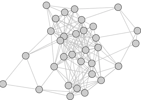
European parliament members

(Thurner et al., 2013)

Induced subgraph from the Dutch members of the European parliament (MEP) in the 6th legislative period (the whole network consists of 900 vertices). Two MEPs are connected if they have at least one committee membership in common.

(19)

1.2 Contributed Manuscripts and Software

Facebook

(McAuley and Leskovec, 2012)

No. of nodes: 4,039 No. of existing edges: 88,234 No. of possible edges: 8,154,741 Network density: 0.01

Combined Facebook friendship data from ten ego-networks (an ego-net is the network among friends of a certain actor who is the ego, the ego itself is by definition connected to every other vertex in his ego-net).

1.2 Contributed Manuscripts and Software

1.2.1 Contributed Manuscripts

This thesis contains parts which are already published as stand-alone articles or available as online pre-prints, and which are joint work with co-authors. For the Bayesian approach in Chapter 3 this is

Thiemichen, S., Friel, N., Caimo, A., and Kauermann, G. (2016). Bayesian exponential random graph models with nodal random effects.

Social Networks, 46:11–28.

The subsampling and the non-parametric extension in Chapter 4 corresponds to

Thiemichen, S. and Kauermann, G. (2016). Stable exponential random graph models with non-parametric components for large dense networks.

arXiv preprint arXiv:1604.04732.

(20)

1 Introduction

1.2.2 Software

All computations and most figures in this work have been produced using the R system for statistical computing (R Core Team, 2016), version 3.3.0 (if not stated otherwise), with packages ergm 3.6.0, network 1.13.0, and statnet.common 3.3.0. Information on additional add-on packages and our implemented routines is included at the beginning of the corresponding chapters. Our algorithms developed for model fitting and model selection in the Bayesian context in Chapter 3 will be included in theBergmpackage (Caimo and Friel, 2014). The non-parametric approach together with the subsampling scheme in Chapter 4 is available in the package ergam on github (https://github.com/sthiemichen/ergam). All of our implementations are open-source software and therefore free to use for researchers and other users.

For the illustrative graphics in Chapter 2 and the appendix, and the model overview in Chapter 3 Inkscape (The Inkscape Team, 2015) has been used. The visualisation of the Facebook network data example in Chapter 4 has been generated using visone (Brandes and Wagner, 2004).

The picture on the title page shows the author’s personal Facebook friendship network (as of 11th June 2012). The plot has been created using gephi (Bastian et al., 2009). The size of each vertex is proportional to the corresponding nodal degree.

(21)

2 Exponential Random Graph Models

2.1 From Random Graph to Exponential Random Graph

Models

Various stochastic approaches have been proposed to model the adjacency matrix Y of a network consisting ofn nodes. One of the earliest and simplest models is the one suggested by Gilbert (1959). It is usually known as Bernoulli Random Graph Model. The model has the following form for the probability that an edge exists between nodei and node j:

P

Yij = 1

=π, ∀i, j ∈ {1, . . . , n}, and j > i, (2.1)

with π ∈(0,1). This model can be seen as a baseline or intercept-only model. For a large number of nodesn this formulation is equivalent to the model of Erdős and Rényi (1959), where all possible graphs for a given number of nodes n and a given number of existing edgesnE get the same uniform probability.

Extending this formulation to more realistic models lead to the so-calledp1 model (Holland and Leinhardt, 1981). It can be written as

logith_PYij = 1

i

= log





 P

Yij = 1

1−_PYij = 1







=αi +αj +ztijβ, (2.2)

wherezij denotes a set of covariates relating to the vertices iand j, andαi andαj are fixed nodal effects. The difference in thep2 model (van Duijn et al., 2004; Zijlstra et al., 2006)

logith_PYij = 1|φ

i

=φi+φj +ztijβ, (2.3)

φ=φ1, . . . , φn

t

∼N0, σ_φ2In

withIn as n dimensional unit matrix, is the treatment of the node-specific effects as nodal random effectsφi, i= 1, . . . , n, which are considered to be latent and non-observable. This allows to tackle the problem of an increasing number of parameters with increasing number of nodes n in a rather elegant manner, as in most cases the nodal effects themselves are not of interest but only their variance parameter σ2

(22)

2 Exponential Random Graph Models

treated as homogeneous but as heterogeneous.

One of the main advantages of all previously mentioned models is that they fall into the classical generalized linear (mixed) model framework with binomial response and logit link function. Estimation can be carried out with available standard statistical software. When dealing with the p2 model, a Bayesian approach can be used, as in a Bayesian framework including the additional normal distribution assumption needed for the random effects

φi, i = 1, . . . , n, is straightforward via a prior distribution, see, e.g., Gill and Swartz

(2004).

The class of so-called stochastic block models (see, e.g., Snijders and Nowicki, 1997; Nowicki and Snijders, 2001) are another extension of the Bernoulli model (2.1) and similar to thep2 model. In these models, vertices are assigned to latent groups, which are also called blocks. Vertices belonging to the same block get the same probability for forming a tie among themselves, that is usually higher than the probability assigned to vertices belonging to different blocks. The probabilities can vary from block to block, and the block structure is usually unknown and therefore needs to be estimated as well. There are various extensions available, e.g., for considering mixed-memberships of vertices, that is vertices can be belong to more than one block (Airoldi et al., 2008). Stochastic block models are applicable to large networks (see, e.g., Daudin et al., 2008). The same is true for the p2 model. The concept of latent variables in stochastic block models has also been generalized in so-called latent network models (see, e.g., Hoff et al., 2002; Krivitsky and Handcock, 2008).

In all models presented so far, the probability that an edge exists between nodes i and

j does not depend on the network structure itself. Let us consider the concrete example of friendship networks. When trying to model the probability that two actors become friends with each other, considering the number of friends the two have in common is usually a reasonable thing to do (the phenomenon is known as triangulation). Including this additional covariate structure is possible in the Exponential Random Graph Model (ERGM), which is sometimes denoted as p∗ (p-star) model, and has been proposed by Frank and Strauss (1986).

2.2 Properties of Exponential Random Graph Models

By employing Exponential Random Graph Models we use the likelihood function to model the network Y

P

Y =y|θ=fy|θ= exp

n

θts(y)o

κθ , (2.4)

(23)

2.2 Properties of Exponential Random Graph Models

where θ = θ0, . . . , θp

t

denotes the vector of model parameters and s(y) =

s0(y), . . . , sp(y)

t

is a vector of network statistics. It is easy to see that an exponential family is assumed. Therefore, the vector of network statisticss(y) is sufficient, withθbeing the vector of natural or canonical parameters. For more details of exponential families and the associated properties see, e.g., Appendix A.1 of Fahrmeir and Tutz (2001). The vector

s(y) can contain counts of edges, 2-stars, triangles, cycles or other structures (sub-graphs) in the network, see, e.g., Snijders et al. (2006). Figure 2.1 illustrates some of these possible network sub-graphs for an undirected network. Section A.1 in the appendix contains further examples and the corresponding formulae. In addition, it is also possible to incorporate available covariate information like, for instance, counts of edges between actors having the same gender, or who went to the same school. For a comprehensive and a bit more technical overview on model specification of ERGMs see Morris et al. (2008).

When including only structural terms, likek-stars and triangles, the resulting Exponential Random Graph Model has a Markovian independence structure, that is two edges are conditionally independent, given the rest of the network, if they do not share a node (Frank and Strauss, 1986; Whittaker, 2009; Koskinen and Daraganova, 2013). Literally speaking, this results in a dyad depending only on its direct neighbouring dyads (i.e. they share at least one node). For ERGMs containing cycles (4-cycles or higher cycles), k-triangles, or other more complex structures this property does not hold, see Section 4.1, and Section A.2 in the appendix. For an overview of induced dependence structures depending on the specified ERGM we refer to Pattison and Snijders (2013), and the references therein.

Figure 2.1 Examples of network sub-graphs: Edge (1-star), 2-star, 3-star, and triangle.

The term κθ in (2.4) denotes the normalizing constant of the exponential family, that is

κθ= X

y∈Y

expnθts(y)o.

(24)

normalizing constant

∂

∂θ log

κ(θ)=_Es(Y)|θ (2.5)

and

∂2

∂θ∂θtlog

κθ= Covs(Y), s(Y)t|θ. (2.6)

Both expressions can therefore be estimated based on a sample of graphs coming from this ERGM with parameters θ. More details on estimation and simulation are given in the next section.

Model (2.4) can be rewritten in a conditional form

logith_PYij = 1|Ykl,(k, l)6= (i, j);θ

i

=θt sij(y), (2.7)

where sij(y) denotes the vector of so called change statistics

sij(y) = ∆ijs(y) =s

yij = 1, ykl,(k, l)6= (i, j)

−syij = 0, ykl,(k, l)6= (i, j)

.

The change statistics reflect the difference in counts of edges, 2-stars, triangles and so on, which occur between toggling the edge yij from existent to non-existent given the rest of the network. This formulation allows for a rather straightforward conditional interpretation focusing on a single edge Yij. Some statistics are easy to interpret especially using this conditional framework. For instance, if we include the number of triangles in the model, the triangle change corresponds to the number of common friends node iand j have, given the rest of the network, and the parameter θtriangles is accordingly the linear effect of one additional common friend on the log-odds of becoming friends, keeping all other covariates constant. Note that some structural covariates are much harder to interpret. We will give some examples in Section 2.4.

This conditional formulation of the ERGM in (2.7) also shows the similarity to the p1 and

p2 formulations in (2.2) and (2.3), respectively. Note that, as we are including structural network terms, the single observations Yij are not (conditionally) independent here. There is an exception, of course, if we employ an intercept-only model. If we only include the total edge count, the edge change is always one per edge variable and the linear predictor in (2.7) consists only of θ0, which captures the overall tendency of any dyad of forming a tie in the network. In this case the model is equivalent to the Bernoulli Random Graph Model in (2.1).

For a more detailed discussion of properties of Exponential Random Graph Models, we refer to Robins et al. (2007a), Robins et al. (2007b), and Lusher et al. (2013).

(25)

2.3 Estimation of Exponential Random Graph Models

2.3.1 Overview of Estimation Routines

There is a variety of estimation approaches available in the context of Exponential Random Graph Models. The following descriptions are by far not exhaustive. In the frame of this work, only a general overview and a sketch of the most prominent approaches are provided. For a deeper discussion of the algorithms we refer to Hunter et al. (2012), and Koskinen and Snijders (2013).

Pseudo-Likelihood Estimation

One of the simplest approaches for estimation of model (2.4) is the Pseudo-Likelihood estimation (Strauss and Ikeda, 1990). The conditional probability in (2.7) is evaluated for each edge variable Yij, for i, j ∈ {1, . . . , n} and j > i, given the rest of the network. The product of the conditional probabilities

Y

i,j∈{1,...,n}

j>i

P

Yij = 1|Ykl,(k, l)6= (i, j);θ

is used as an approximation of the likelihood. In other words, the dependence structure of the link variables is ignored and the estimation is carried out similar to every standard logistic regression model. Note that the Maximum Pseudo-Likelihood Estimator (MPLE) is an unbiased estimator if the link variables are conditionally independent, which is the case in thep1,p2, and Bernoulli framework, where no structural network effects are considered. Lubbers and Snijders (2007), as well as van Duijn et al. (2009) have shown that the MPLE is biased in most scenarios. Even though there are approaches to correct for this bias using the Fischer information (see Firth, 1993), there is a loss in efficiency compared to the maximum likelihood estimator.

Stochastic Approximation (Robbins-Monro)

(26)

only of a single simulated graph based on the current estimate of θ(t). For the iterative procedure an initial guess for the value of θ is needed. This starting value θ(0) can be obtained using, for instance, the MPLE. The iterative updating from θ(t) toθ(t+1) is done using a Newton-Raphson-type procedure, that is

θ(t+1) =θ(t)−a(t)D−01

s(y(t)−s(y),

where D0 is a scaling matrix. D0 is determined in an initialisation phase as the diagonal of an estimated covariance matrix of the sufficient statistics based on some graph samples (compare to equation (2.6)) using θ(0). The term a(t) denotes a step length between zero and one, which becomes smaller in each iteration and is needed to avoid “overshooting” of the MLE. For more details on the stochastic approximation approach see, e.g., Koskinen and Snijders (2013).

MCMC MLE (Geyer-Thompson)

Handcock (2003), and later Hunter and Handcock (2006) adopted an alternative for the computation of the maximum likelihood estimator in ERGMs, the MCMC MLE of Geyer and Thompson (1992). This approach is sometimes referred to as “importance sampling”. Instead of maximizing the likelihood directly, the likelihood ratio is considered, which results in the log-likelihood formulation

`θ−`θ0

=θ−θ0

t

s(y)−log







κθ

κθ0







. (2.8)

Again, by default, the easy to calculate MPLE can be used as a starting value θ0 to generate an initial sample of graphs from an ERGM based on the valueθ0. Then, the ratio of normalizing constants

κθ

κθ0

=E

exp

θ−θ0

t

s(Y)|θ0

is approximated based on this sample. This allows to maximize the log-likelihood (2.8) as a function of the parameters θ, which are of interest. The goal is to get an expected value of the statistics_E(s(Y)), which is approximated using the initial sample of graphs, as close as possible to the observed value of the statistics s(y) by iteratively updating the estimate of θ to θ(t+1), again, using a Newton-Raphson-type equation. Note that in each step only the initial sample of graphs is used. Problems usually arise when the initial value of θ0 is not close enough to the true parameter vector θ, sometimes even resulting in an expression which cannot be maximized at all, see, e.g., Figure 2 of Hunter et al. (2008b), or Figure

(27)

2.3 Estimation of Exponential Random Graph Models

3 of Caimo and Friel (2011). The algorithm can then be restarted (including new initial simulations of graphs) with other initial values, obtained either as the last estimate from the previous run, or completely new ones specified by the user. Nevertheless, approximation of a ratio of such normalizing constants is in general much more stable than approximating one of them directly.

Other Approaches

Caimo and Friel (2011) propose a Bayesian framework which is based on the exchange algorithm of Murray et al. (2006) and circumvents the calculation of normalizing constants completely. This approach is described in more detail in Section 3.2. Again, simulations of networks are needed to employ this strategy. A common method for network simulation from an ERGM is described in the next subsection.

The stochastic approximation approach (Robbins-Monro algorithm) is less prone to bad initial values than the MCMC MLE (Geyer-Thompson algorithm). Therefore, in general, it is quite robust, even though it is less efficient than the MCMC MLE, where only an initial sample of graphs is needed. The non-Bayesian ERGM estimation approaches described so far are, e.g., available in the R package ergm (Hunter et al., 2008b), which is also part of the statnetsuite of packages (Handcock et al., 2008).

There are several extensions and suggestions for improvements of estimation in the ERGM framework available, e.g., by Hummel et al. (2012). For a more detailed description of available estimation routines and extensions we refer to the survey article of Hunter et al. (2012), the book of Lusher et al. (2013), and the references therein.

2.3.2 Network Simulation

(28)

y_proposed. The toggle is accepted with probability

α= min







1,P

Y =y_proposed|θ∗ P

Y =y_current|θ∗ 



 ,

where the needed probabilities result from the ERGM with parameter vector θ∗. Note that in the probability ratio in α the normalizing constants simply cancel out, as they are identical for both probabilities _PY = y_proposed|θ∗ and _PY = y_current|θ∗. The TNT in the ergm package does not select edge variables uniformly at random, but uses a probability of 0.5 to select an edge variable which is currently zero. This normally leads to faster convergence of the Markov chain, which is more effective in sparse settings, as less iterations are needed for simulating a single network, see Morris et al. (2008), and Hunter et al. (2008b) for details.

Often, if several simulated networks based on the same parameters are needed, a single Markov chain is used, allowing the chain to burn-in (the burn-in is the number of iterations before the first network is stored from the chain) and using a smaller number of interval iterations between the successive draws. This is usually more efficient than employing several chains, each starting from scratch, and each of them providing a single simulated network only. The resulting draws are correlated in this case. There are some diagnostic tools and theoretical results available concerning the number of iterations needed to obtain a draw from the target distribution when simulating a network. The chain generating the network samples needs a sufficiently large burn-in and the number of iterations between each successively generated network using this chain should be large enough as well. Checking the autocorrelation of successive draws is an option to see if enough interval iterations are used, see, e.g., Koskinen and Snijders (2013). The autocorrelation should not be too high. Looking at trace plots of counts of network statistics (e.g., edges, 2-stars, or triangles) can help to identify a sufficiently large burn-in. Following Everitt (2012), in the Bayesian framework (Caimo and Friel, 2011) it is often sufficient to use roughly the number of possible ties in the network as number of iterations of the Markov chain to obtain a single network. In general, the extensive number of simulations needed in estimation of ERGMs is one of the main causes of the computational burden associated with this model class.

2.3.3 Goodness-of-Fit

Goodness-of-fit (GOF) assessment of Exponential Random Graph Models is usually obtained based on samples of graphs simulated from the fitted model. Hunter et al. (2008a) proposed to consider network statistics like, e.g., the distributions of degree, edge-wise-shared partners (for existing edges the number of common neighbours of the two vertices involved), or geodesic distance (the shortest path length between two nodes), and compare

(29)

2.4 Challenges and Solutions

them graphically between the sampled networks and the original network (see also Robins et al., 2007b). The statistics do not necessarily have to be included as model terms in the fitted ERGM. If the observed values fall in the range of the simulated ones, it is an indicator that the model is suitable for these data aspects. If this is not the case, the model is not capable of capturing some data properties. However, there is often no direct indication why the model performs badly and how to proceed in order to improve model fit. We employ this classical GOF procedure in the Bayesian framework in Section 3.4.1. As can be seen here, this approach for assessing model fit follows different routes than traditional likelihood based inference, such as likelihood ratio tests, etc.. This is due to the fact that the likelihood itself is difficult to evaluate because of the aforementioned problems implied by the unknown normalizing constant. For an overview of more classical type testing routines in ERGMs, see Koskinen and Snijders (2013).

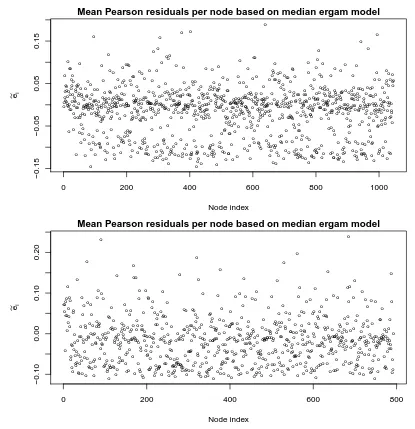
In Chapter 4, we employ Pearson residuals as an additional diagnostic tool, which allows us to identify at least some potential problems causing difficulties in model fit.

2.4 Challenges and Solutions

2.4.1 Degeneracy

Apart from the already mentioned computational drawbacks for MLE estimation in the Exponential Random Graph framework due to extensive MCMC based routines, the model class suffers from so-called degeneracy problems, see, for instance, Snijders et al. (2006), Schweinberger (2011), and Chatterjee and Diaconis (2013). This means that for a lot of parameter values θ, most of the probability mass is placed on configurations yielding completely empty or completely full graphs. As pointed out before, the maximum likelihood estimation routines are simulation based and hence, generating only empty or full graphs is problematic. The remaining parameter space resulting in reasonable networks is often peculiarly shaped and small, see, e.g., Handcock (2003), Rinaldo et al. (2009), and Schweinberger (2011). A lot of basic models which are usually appealing because of the easy to interpret effects, e.g., the ones containing only 2-stars, or higher k-stars, or triangles, show near-degenerate behaviour. To illustrate the issue we simulate networks with n= 30 nodes from an Exponential Random Graph Model with edge and 2-star statistics, i.e.

P

Y =y|θ= exp

n

θedge sedge(y) +θ2-star s2-star(y)

o

κθ .

(30)

−1.0 −0.5 0.0 0.5 1.0

0.0

0.2

0.4

0.6

0.8

1.0

ERGM with θedge (= −2) and θ2−star

θ2−star

A

v

er

age netw

or

k density (f

or 30 node netw

or

k)

Figure 2.2 Resulting average network density when simulating graphs with n= 30 nodes from an ERGM containing edge and 2-star counts.

network is calculated as the number of existing edges divided by the number of possible edges d(y) = nE/

_n(n₋₁₎

2

. The corresponding R code for the simulation can be found in Appendix B. The sharp transition from a rather sparse to a full graph for only a small change of the value of θ2-star is apparent. This transition becomes even sharper with increasing n, which results in the region of parameter values yielding reasonable graphs becoming even smaller.

For an ERGM containing edges, 2-stars, and triangles as sufficient statistics, Schweinberger (2011) has shown that only a linear combination of the form

θ2-star =−

θtriangle

3 (2.9)

results in a stable setting, that is the obtained graphs are not completely full or completely empty, independently of the value of n. This result is in line with the often stated practical recommendation of compensating a positive triangle effect with a small negative 2-star effect. Figure 2.3 illustrates the stable setting in (2.9). We see that there still is a transition, but clearly less sharp and not resulting in completely full graphs. When assuming this setting for model estimation, only one parameter remains to be estimated. When doing so,

(31)

−1.0 −0.5 0.0 0.5 1.0

0.0

0.2

0.4

0.6

0.8

1.0

ERGM with θedge (= −2), θ2−star and θtriangle

θ2−star = − θtriangle 3

A

v

er

age netw

or

k density (f

or 30 node netw

or

k)

Figure 2.3 Resulting average network density when simulating graphs with n = 30 nodes from

an ERGM containing edge, 2-star, and triangle counts withθ2-star =−θtriangle₃ .

the resulting combined statistic1 is not straightforward to interpret.

Caimo and Friel (2011) have shown that the Bayesian Exponential Random Graph Model behaves more stable in near-degenerate situations, where estimation in the standard ERGM already breaks down.

2.4.2 Geometrically Weighted Statistics

The instability appearing in Exponential Random Graph Models has led to the proposal of modified statistics as, for instance, alternating star or alternating triangle statistics (Snijders et al., 2006). From a modelling point of view, the geometrically weighted degree (GWD) statistic

eθdec

n−1

X

i=1

1−1−e−θdeci

Di(y),

1_{When restricting an ERGM containing edges, 2-stars, and triangles to setting (2.9), we obtain}

θ2-star s2-star(y)−3θ2-star striangle(y) =θ2-starscombined(y),

(32)

where Di(y) denotes the number of nodes with degree i, and the geometrically weighted edge-wise shared partners (GWESP) statistic

eθdec

n−2

X

i=1

1−1−e−θdeci

EPi(y),

where EPi(y) denotes the number of edges with i shared partners, are equivalent to the alternating statistics (Hunter, 2007; Goodreau, 2007). Both statistics use an exponential down-weighting of the incorporated counts. The parameter θdec is usually set to some fixed value (the standard choice is log(2)). In the framework of Curved Exponential Family Models (Hunter and Handcock, 2006), the parameterθdec is estimated as well. These types of statistics stabilise the whole model fitting, but are very difficult to interpret.

In Chapter 4, we propose an alternative by adding smooth functional components to the model, based on penalized estimation in the context of non-parametric models (see Ruppert et al., 2003), while maintaining the intuitive interpretability of statistics like 2-stars and triangles.

2.4.3 Nodal Heterogeneity

In ERGMs nodes are assumed to be homogeneous, except for differences captured in available (nodal) covariates. This assumption may be unrealistic, especially in the context of social networks, where some actors tend to attract a lot of connections, while others prefer to stay on their own. This difference can not necessarily be explained completely by covariates, like gender, age, etc.. The modelling approach of the p2 model in (2.3) therefore yields the baseline for our first extension of the ERGM in Chapter 3 by adding nodal random effects to the model, resulting in

logith_PYij = 1|Ykl,(k, l)6= (i, j);θ, φi, φj

i

=θt sij(y) +φi+φj (2.10)

with φ = φ1, . . . , φn

t

and φi i.i.d.

∼ Nµφ, σφ2

, i = 1, . . . , n. The extended model falls

in the general class of Exponential-family Random Network Models, proposed by Fellows and Handcock (2012). Krivitsky et al. (2009) also develop a model with actor-specific random effects based on a latent cluster model. We follow this line of thought and add interpretability of the approach by considering the parameter σ2

φ as a measure of nodal heterogeneity. There is a connection between the nodal random effects φi, i = 1, . . . , n and the nodal degrees, as these are the statistics associated with the random effects, which is explained in greater detail in Section 3.1. This interpretation is related to the work of Snijders (1981), where the author uses the degree variance as a measure of graph heterogeneity.

(33)

2.4.4 Further Limitations

Another issue arising when dealing with Exponential Random Graph Models is that these models are not consistent under sampling (Shalizi and Rinaldo, 2013). If we are interested in a population of, e.g., n∗ nodes, but we only have data on the induced sub-graph of n

nodes, wheren < n∗, fitting an ERGM to the sub-graph does not give reasonable estimates for the whole network of n∗ nodes. This whole issue comes back to the notion of n, the number of nodes, being fixed when fitting an Exponential Random Graph Model. It implies that parameter estimates resulting from ERGMs fitted to networks with a different number of nodes are not directly comparable. One should keep this in mind when interpreting the model outcomes. This problem limits the generalisability of results obtained from Exponential Random Graph Models to a greater population when only data on a sample was available for model fitting.

The issue of missing data in the network context is a topic of its own and not specific to Exponential Random Graph Models. However, there are a few approaches available in context of ERGMs to cope with edge variables being unobserved, i.e. when there is no information available whether these edges exist or not, see, e.g., the work of Handcock and Gile (2010) in the context of different network sampling designs.

A further limitation is the restriction to the modelling of binary tie variables only. This may cause a loss in information if the available data consists of weighted edges, like for example trade flows, where the amount is recorded and not only whether there was trade between two nodes or not. Krivitsky (2012), and Krivitsky and Butts (2015), or Desmarais and Cranmer (2012a), for instance, propose some strategies for dealing with such valued networks.

Classical Exponential Random Graph Models are static, meaning that they allow to model cross-sectional data. An assumption related to this property is that the network we see comes from its stationary distribution. This assumption can be violated especially if the underlying network-generating process has not settled in already. There are extensions available for modelling longitudinal network data, see, e.g., Snijders et al. (2010a). For a general overview of available approaches in or related to the Exponential Random Graph context we refer to Snijders and Koskinen (2013). Hanneke et al. (2010), for instance, have proposed time discrete models. Another widely used and well developed modelling approach for longitudinal network data are the stochastic-actor oriented models (SAOM; see, e.g., Snijders, 2001; Snijders et al., 2010b). They are not tie oriented as the ERGMs, but the main difference lies in the SAOM focusing on the changes occurring during two points in time. Consequently, stationarity of the underlying process is not assumed.

(34)

(35)

3 Bayesian Exponential Random Graph

Models with Nodal Random Effects

Abstract

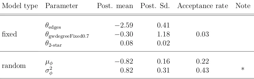
We extend the well-known and widely used Exponential Random Graph Model (ERGM) by including nodal random effects to compensate for heterogeneity in the nodes of a network. The Bayesian framework for ERGMs proposed by Caimo and Friel (2011) yields the basis of our modelling algorithm. A central problem in network models is the question of model selection and following the Bayesian paradigm we focus on estimating Bayes factors. To do so we develop an approximate but feasible calculation of the Bayes factor which allows to pursue model selection. Three data examples and a small simulation study illustrate our mixed model approach and the corresponding model selection.

Contributed Manuscript

This chapter is in most parts equivalent to the final submitted version of the publication

Thiemichen, S., Friel, N., Caimo, A., and Kauermann, G. (2016). Bayesian exponential random graph models with nodal random effects.

Social Networks, 46:11–28.

except for a few corrections, mainly concerning orthography, and small adjustments as the paper serves as a chapter in this thesis and no longer as stand-alone article.

(36)

3 Bayesian Exponential Random Graph Models with Nodal Random Effects

Alberto Caimo helped with code debugging. Most of the manuscript was written by Stephanie Thiemichen, and Göran Kauermann. All authors contributed to the discussion section of the article, and were involved in proof-reading the manuscript.

Software

All computations and plots in this chapter have been produced using R version 3.2.2 with packages Bergm 3.0.1, mvtnorm 1.0-3, coda 0.18-1, ergm 3.5.1, network 1.13.0, and statnet.common 3.3.0. For parallelisation of the simulation and for the Bayes factor computation R’s base package parallel was used, where possible.

Our algorithms for model fitting and model selection will be included in theBergmpackage.

The graphical model overview in Figure 3.1 has been generated using Inkscape (version 0.48.4).

(37)

3.1 Introduction

The analysis of network data is an emerging field in statistics which is challenging both model-wise and computationally. Recently Goldenberg et al. (2010), Hunter et al. (2012), Fienberg (2012), and Salter-Townshend et al. (2012), respectively, published comprehensive survey articles discussing statistical approaches, challenges and developments in network data analysis. We also refer to the monograph of Kolaczyk (2009) for a comprehensive introduction to the field.

In this chapter we consider networks represented as an×n dimensional adjacency matrix

Y, where the element Yij = 1, if an edge exists between vertex i and vertex j, and Yij = 0 otherwise, with i, j ∈ {1, . . . , n} and i 6= j, that is there is no connection from a vertex to itself. With n we denote the number of vertices in the network and for simplicity we assume undirected edges, that is Yij = Yji. Therefore, the matrix Y is symmetric and for simplicity it is sufficient to consider the upper triangle of Y only, that is Yij, j > i. Our approach equally applies to non-symmetric adjacency matrices corresponding to directed graphs. A concrete realisation ofY is denoted with y.

With respect to the available statistical models for modelling cross-sectional network data one may roughly distinguish between two strands, (a) models which explain the existence of an edge purely with external nodal covariates or random effects and (b) models where the existence of an edge also depends on the local network structure. The first strand of models is phrased as p1 and p2 models tracing back to Holland and Leinhardt (1981). Specifically, in thep1 model we set

logith_PYij = 1

i

= log





 P

Yij = 1

1−_PYij = 1







=αi +αj +ztijβ, (3.1)

wherezij denotes a set of covariates relating to the verticesiandj and αi andαj are nodal effects, here assuming undirected edges. Since the number of parameters increases with increasing network size n, van Duijn et al. (2004) proposed to replace the α parameters in (3.1) by random effects, see also Zijlstra et al. (2006). This yields thep2 model

logith_PYij = 1|φ

i

=φi+φj +ztijβ, (3.2)

φ=φ1, . . . , φn

t

∼N0, σ_φ2In

with In as n dimensional unit matrix. A general principle with this approach is that vertices (or actors in the network, respectively) are not considered as homogeneous but heterogeneous, though their heterogeneity is not observable but latent and expressed in the node specific random effects φi, i= 1, . . . , n.

(38)

framework which allows estimation using standard statistical software. The p2 models also allow for Bayesian estimation approaches, see for example Gill and Swartz (2004).

The second strand in statistical network modelling is based on the so called Exponential Random Graph Model (ERGM) proposed by Frank and Strauss (1986). Here we model directly the network using the likelihood function

P

Y =y|θ=fy|θ= qθ

y

κθ =

expnθts(y)o

κθ , (3.3)

whereθ =θ0, . . . , θp

t

is the vector of model parameters ands(y) =s0(y), . . . , sp(y)

t

is a vector of sufficient network statistics like the number of edges or 2-stars in a network, see for example Snijders et al. (2006). In equation (3.3) the termκθdenotes the normalizing constant, that is

κθ= X

y∈Y

expnθts(y)o

and is accordingly the sum over 2(n2) potential undirected graphs and therefore numerically intractable, except for very small graphs. Early fitting approaches are based on the Pseudo-Likelihood idea proposed by Strauss and Ikeda (1990). More advanced are MCMC based routines proposed by Hunter and Handcock (2006) based on the work of Geyer and Thompson (1992). A fully Bayesian approach to estimate ERGMs has been developed by Caimo and Friel (2011).

Model (3.3) allows for a conditional interpretation by focusing on the occurrence of a single edge between two nodes. To be specific we obtain

logith_PYij = 1|Ykl,(k, l)6= (i, j);θ

i

=θt sij(y), (3.4)

where sij(y) denotes the vector of so called change statistics

sij(y) =s

yij = 1, ykl,(k, l)6= (i, j)

−syij = 0, ykl,(k, l)6= (i, j)

.

We refer to Robins et al. (2007a), Robins et al. (2007b), and the rather recent work of Lusher et al. (2013) for a deeper discussion of Exponential Random Graph Models.

Contrasting equation (3.4) with the p1 and p2 model given in equations (3.1) and (3.2) it becomes obvious that the ERGM in contrast to the p1 and p2 models take the network structure into account while considering the nodes to be homogeneous. When modelling network data this means that all possible heterogeneity in the network nodes (that is the actors in the network) is included as covariates in the model and influence the (global) structure of the network. Since homogeneity of the nodes have led from p1 top2 models, we want to pursue the same modelling exercise by allowing for latent node specific heterogeneity

(39)

3.1 Introduction

in Exponential Random Graph Models. To do so, we combine thep2 model (3.2) with the ERGM (3.4) towards

logith_PYij = 1|Ykl,(k, l)6= (i, j);θ, φi, φj

i

=θt sij(y) +φi+φj (3.5)

with φ = φ1, . . . , φn

t

and φi i.i.d.

∼ Nµφ, σ2φ

, i = 1, . . . , n. The parameter µφ captures

the average propensity in the network for forming a tie. Therefore θ0, which is usually the parameter associated with the edges statistic, is excluded fromθ, i.e.θ =θ1, . . . , θp

t

here. In terms of the likelihood function for the whole network we obtain from (3.5)

P

Y =y|θ,φ=fy|θ,φ= qθ,φ

y

κθ,φ =

expnθts(y) +φtt(y)o

κθ,φ , (3.6)

where t(y) contains the degree statistics of the n vertices, i.e. ti(y) = n

P

j=1

yij, for i =

1, . . . , n. That is we fit an Exponential Random Graph Model with random, node specific

effects accounting for heterogeneity. The model in equations (3.5) and (3.6) falls in the general class of Exponential-family Random Network Models proposed by Fellows and Handcock (2012) but unlike their model we treat the node specific effect as latent and we pursue a fully Bayesian estimation. We also refer to Krivitsky et al. (2009) who propose a model with actor specific random effects based on a latent cluster model. The authors also propose node specific random effects. We follow this line and give further interpretability of the effects. A central issue in model extensions is the question of model selection. We emphasize this point in this work by comparing models with and without nodal effects using the Bayes factor as model selection criterion. However, calculation of the Bayes factor suffers from the above mentioned problem in Exponential Random Graph Models in that the normalization constantκ· is numerically infeasible. We therefore propose an approximate calculation of the Bayes factor and show in a simulation study its usability for model selection.

For estimation and model selection of model (3.6) we extend the fully Bayesian approach from Caimo and Friel (2011). The developed estimation routine is based on the numerical work of Caimo and Friel (2014) with their R (R Core Team, 2016) package Bergm (see http://cran.r-project.org/web/packages/Bergm). Our algorithms for model fitting and selection will be included in the Bergm package.

(40)

3.2 Bayesian Model Formulation and Estimation

Before proposing a fully Bayesian formulation for model (3.6) bear in mind that the normalizing constantκθ,φis numerically infeasible to calculate except for small networks so that numerically demanding simulation based fitting routines need to be employed. We follow a fully Bayesian approach by imposing a prior distribution on θ = θ1, . . . , θp

t

. The posterior of interest for the Bayesian Exponential Random Graph Model with nodal random effects in (3.6) then becomes

pθ,φ, µφ, σφ2|y

= f

y|θ,φpθpφ|µφ, σ2φ

pµφ

pσ2

φ

py , (3.7)

where pθ is the prior distribution of θ and pφ|µφ, σ2φ

the prior for the random nodal effects φ. We assume the nodal effects to be independent and identically normally distributed, that is

φi ∼N

µφ, σφ2

, for i= 1, . . . , n

and accordingly we use θ ∼ N0, ρ2_I p

, with Ip denoting the p-dimensional unity matrix

andρ2 _{chosen such that the prior distribution is flat. For the hyper prior distribution}_p_µ φ

of the mean µφ we assume a normal distribution centred at 0, that is

µφ∼N

0, τ2.

The hyper prior pσ2 φ

of the variance σ2

φ is assumed to be an inverse gamma distribution, that is

σ2_φ∼IGa, b.

Finally, the parameters τ2_, _a _and _b _{are all constants and chosen in a way that results in} flat hyper prior distributions. Figure 3.1 illustrates this Bayesian model formulation.

It is important to note, that the posterior distribution in (3.7) is so-called doubly-intractable. This is because, firstly, it is not possible to evaluate the posterior density (3.7) due to py, the marginal likelihood or evidence, being intractable. Secondly, it is

also numerically infeasible to calculate the normalizing constant κθ,φ in the likelihood

fy|θ,φ except for very small network graphs. Similar to the algorithm proposed by Caimo and Friel (2011) we use the so-called exchange algorithm from Murray et al. (2006) to draw samples from the posterior distribution of interest. Let therefore γ = θt,φtt

denote the entire parameter vector of the ERGM. Instead of drawing directly from (3.7),

(41)

3.2 Bayesian Model Formulation and Estimation

Figure 3.1 Overview of the Bayesian model formulation for the Exponential Random Graph Model with nodal random effects.

we sample from the augmented distribution

pγ0,y0,γ, µφ, σ2φ|y

∝

fy|γpγ|µφ, σ2φ

pµφ

pσ_φ2hγ0|γfy0|γ0, (3.8)

where h·|· is a proposal function, to be specified later. This proposal provides γ0 =

θ0t,φ0tt as new candidate values for θ and φ, respectively, and based on γ0 we can simulatey0 as an auxiliary network. The proposal is accepted with probability

α= min



1,

qγ

y0pγ0hγ|γ0qγ0

y

qγ

ypγhγ0_|_γ_q

γ0

y0 ×

κγκγ0



, (3.9)

where pγ =pθ·pφ|µφ, σ2φ

(42)

Friel (2011) it is advisable to separate the proposals ofθandφto achieve higher acceptance rates. This is described in the following algorithmic steps. In detail, our algorithm works as follows:

Algorithm 1: Fit BERGM with nodal random effects

Step 1: Gibbs update of (θ0,y0): (i) Draw θ0 ∼h·|θ. (ii) Draw y0 ∼p·|θ0,φ.

(iii) Propose to move fromθ toθ0 with probability

α= min



1,

qθ,φ

y0pθ0hθ|θ0q_θ0_,_φ

y

qθ,φ

ypθhθ0|θqθ0,φ

y0 ×

κθ,φκθ0,φ



.

Step 2: Gibbs update of (φ0,y0): (i) Draw φ0 ∼g·|φ. (ii) Draw y0 ∼p·|θ,φ0.

(iii) Propose to move fromφ toφ0 with probability

α= min



1,

qθ,φ

y0pφ0|µφ, σφ2

gφ|φ0qθ,φ0

y

qθ,φ

ypφ|µφ, σφ2

gφ0|φqθ,φ0

y0 ×

κθ,φκθ,φ0



.

Step 3: Metropolis-Hastings update of µφ: Draw proposal µ0_φ fromk·|µφ

and accept the proposed value with probability

α= min



1,

pφ|µφ, σ2φ

pµφ

pφ|µ0

φ, σ2φ

pµ0

φ



.

Step 4: Metropolis-Hastings update of σ2_φ: Draw proposal σ2

φ

0

from l·|σ2 φ

and accept the proposed value with probability

α= min



1,

pφ|µφ, σ2φ

pσ2

φ

pφ|µφ, σ2φ

0

pσ2

φ

0 

.

Start again with Step 1 until the maximum number of iterations is reached.

Thiemichen, Stephanie (2016): Extensions of exponential random graph models for network data analysis. Dissertation, LMU München: Fakultät für Mathematik, Informatik und Statistik

Stephanie Thiemichen

Extensions of Exponential Random

Graph Models for Network Data

Analysis

Stephanie Thiemichen

Extensions of Exponential Random

Graph Models for Network Data

Analysis

Dissertation an der Fakultät für Mathematik, Informatik und Statistik

der Ludwig-Maximilians-Universität München

Erster Berichterstatter: Prof. Dr. Göran Kauermann

Zweiter Berichterstatter: Prof. Dr. Ernst Wit

Danksagung

Danksagung

Zusammenfassung

Summary

Contents

1 Introduction

1.1 Data Examples

1.2 Contributed Manuscripts and Software

1.2.1 Contributed Manuscripts

1.2.2 Software

2 Exponential Random Graph Models

2.1 From Random Graph to Exponential Random Graph

Models

2.2 Properties of Exponential Random Graph Models

2.3 Estimation of Exponential Random Graph Models

2.3.1 Overview of Estimation Routines

2.3.2 Network Simulation

2.3.3 Goodness-of-Fit

2.4 Challenges and Solutions

2.4.1 Degeneracy

2.4.2 Geometrically Weighted Statistics

2.4.3 Nodal Heterogeneity

2.4.4 Further Limitations

3 Bayesian Exponential Random Graph

Models with Nodal Random Effects

3.1 Introduction

3.2 Bayesian Model Formulation and Estimation