Electronic Thesis and Dissertation Repository
4-1-2011 12:00 AM
Confidence Interval Estimation for Continuous Outcomes in
Confidence Interval Estimation for Continuous Outcomes in
Cluster Randomization Trials
Cluster Randomization Trials
Julia Taleban
The University of Western Ontario
Supervisor
Dr. Guang Yong Zou
The University of Western Ontario Graduate Program in Biostatistics
A thesis submitted in partial fulfillment of the requirements for the degree in Doctor of Philosophy
© Julia Taleban 2011
Follow this and additional works at: https://ir.lib.uwo.ca/etd
Part of the Biostatistics Commons
Recommended Citation Recommended Citation
Taleban, Julia, "Confidence Interval Estimation for Continuous Outcomes in Cluster Randomization Trials" (2011). Electronic Thesis and Dissertation Repository. 121.
https://ir.lib.uwo.ca/etd/121
This Dissertation/Thesis is brought to you for free and open access by Scholarship@Western. It has been accepted for inclusion in Electronic Thesis and Dissertation Repository by an authorized administrator of
RANDOMIZATION TRIALS
(Spine title: Confidence Intervals in Cluster Randomization Trials)
(Thesis format: Monograph)
by
Julia Taleban
Graduate Program in Epidemiology & Biostatistics
A thesis submitted in partial fulfillment of the requirements for the degree of
Doctor of Philosophy
School of Graduate and Postdoctoral Studies University of Western Ontario
London, Ontario April 27, 2011
c
Supervisor Examining Board
aaaaaaaaaaaaaaaaaaaaaa aaaaaaaaaaaaaaaaaaaaaa
Dr. Guangyong Zou Dr. Neil Klar
Co-Supervisor aaaaaaaaaaaaaaaaaaaaaa
Dr. Duncan Murdoch
aaaaaaaaaaaaaaaaaaaaaa
Dr. John Koval aaaaaaaaaaaaaaaaaaaaaa
Dr. Serge Provost
Committee member
aaaaaaaaaaaaaaaaaaaaaa
Dr. Wendy Lou
aaaaaaaaaaaaaaaaaaaaaa
Dr. Allan Donner
The thesis by Julia Taleban
Entitled
Confidence Interval Estimation for Continuous Outcomes in Cluster Randomization Trials
is accepted in partial fulfillment of the requirements for the degree of
Doctor of Philosophy
Date: aaaaaaaaaaaaaaaaaa aaaaaaaaaaaaaaaaaaaaaaaaaaaaaaaaaaa
Chair of the Thesis Examination Board
pitals, schools, communities, and families) are randomized to the arms of the trial
rather than individuals. The popularity of this design among health researchers is
partially due to reduced contamination of treatment effects and convenience.
How-ever, the advantages of cluster randomization trials come with a price. Due to the
dependence of individuals within a cluster, cluster randomization trials suffer reduced
statistical efficiency and often require a complex analysis of study outcomes.
The primary purpose of this thesis is to propose new confidence intervals for effect
measures commonly of interest for continuous outcomes arising from cluster
random-ization trials. Specifically, we construct new confidence intervals for the difference
between two normal means, the difference between two lognormal means, and the
exceedance probability.
The proposed confidence intervals, which use the method of variance estimates
recovery (MOVER), do not make certain assumptions that existing procedures make
on the data. For instance, symmetry is not forced when the sampling distribution
of the parameter estimate is skewed and the assumption of homoscedasticity is not
made. Furthermore, the MOVER results in simple confidence interval procedures
rather than complex simulation-based methods which currently exist.
Simulation studies are used to investigate the small sample properties of the
MOVER as compared with existing procedures. Unbalanced cluster sizes are
sim-ulated, with an average range of 50 to 200 individuals per cluster and 6 to 24 clusters
per arm. The effects of various degrees of dependence between individuals within the
same cluster are also investigated.
When comparing the empirical coverage, tail errors, and median widths of
confi-dence interval procedures, the MOVER has coverage close to the nominal, relatively
balanced tail errors, and narrow widths as compared to existing procedure for the
Keywords: cluster randomization trials, confidence intervals, normal mean, lognor-mal mean, exceedance probability, method of variance estimates recovery, generalized
confidence interval procedure, Wald method.
support of many people. First, I would like to thank my Ph.D. supervisor, Dr. Guang
Yong Zou, who provided me with invaluable guidance and insight. I would also like
to thank my co-supervisor, Dr. John Koval, whose encouragement and suggestions
have been a great help, and Dr. Allan Donner for the time he took to discuss the
drafts of the thesis and his helpful suggestions.
I am grateful to Dr. Thomas Marrie and Dr. Alan Montgomery for the use of
their datasets while illustrating various confidence interval methods in Chapter 5.
I am indebted to my parents and friends for their moral support and
encourage-ment. My fiance Luc has shown constant support and endless patience, and for that
I am thankful.
This work has been financially supported in part by the Ontario Graduate
Schol-arship in Science and Technology and by the Ontario Graduate ScholSchol-arship from the
Ontario Ministry of Training, Colleges, and Universities.
Certificate of Examination ii
Abstract iii
Acknowledgments v
List of Tables x
List of Figures xiii
Chapter 1 Introduction 1
1.1 Randomized controlled trials . . . 1
1.2 Cluster randomization trials . . . 1
1.3 Notation . . . 5
1.4 Brief summary of methods for cluster randomization trials with con-tinuous data . . . 8
Cluster-level analyses . . . 8
Individual level analyses . . . 9
Current methods for a difference between two normal means . . . 12
1.5 Alternative effect measures in cluster randomization trials . . . 15
The standardized mean difference . . . 15
The difference between two lognormal means . . . 21
1.6 Scope of the thesis . . . 24
1.7 Objectives . . . 26
1.8 Organization of the thesis . . . 27
Chapter 2 Fundamentals of confidence interval estimation 28 2.1 Introduction . . . 28
2.2 Definition of a confidence interval . . . 31
2.3 Confidence interval estimation for a single parameter . . . 32
The inversion principle . . . 32
The transformation principle . . . 33
2.4 Wald-type confidence intervals and the delta method . . . 33
A single parameter . . . 34
A function of multiple parameters . . . 34
Properties of Wald-type confidence intervals . . . 35
Properties of the MOVER . . . 47
Previous applications . . . 49
Chapter 3 Confidence interval estimation for effect measures in clus-ter randomization trials 53 3.1 A difference between two normal means . . . 54
The MOVER . . . 54
Alternative confidence intervals . . . 55
Wald confidence interval . . . 55
Cluster-adjusted confidence interval . . . 56
Generalized confidence interval . . . 57
3.2 A difference between two lognormal means . . . 59
The MOVER for a single mean . . . 59
The MOVER for a difference between two lognormal means . . . 62
Alternative confidence intervals . . . 62
Wald confidence interval and the delta method . . . 62
Generalized confidence intervals . . . 64
3.3 The exceedance probability . . . 65
The MOVER . . . 65
Alternative confidence intervals . . . 66
Wald confidence interval and the delta method . . . 66
Generalized confidence interval . . . 68
Chapter 4 Simulation study of confidence interval procedures 70 4.1 Introduction . . . 70
4.2 Objectives . . . 71
4.3 Methods . . . 72
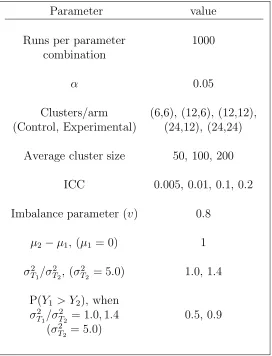
Parameter combinations . . . 72
Data generation . . . 75
Cluster sizes . . . 75
Correlated normal data . . . 77
Correlated lognormal data . . . 78
Computer software for data generation . . . 79
Methods of comparison . . . 79
4.4 Results . . . 80
The difference between two normal means . . . 80
Confidence interval coverage . . . 81
Tail errors . . . 87
Median width . . . 95
The exceedance probability . . . 95
Confidence interval coverage . . . 95
Tail errors . . . 97
Median width . . . 108
4.5 Discussion . . . 108
The difference between two normal means . . . 108
Confidence interval coverage . . . 109
Confidence interval tail errors . . . 110
Confidence interval widths . . . 111
The difference between two lognormal means . . . 111
Confidence interval coverage . . . 112
Confidence interval tail errors . . . 113
Confidence interval widths . . . 114
The exceedance probability . . . 114
Confidence interval coverage . . . 115
Confidence interval tail errors . . . 115
Confidence interval widths . . . 116
4.6 Overall conclusions . . . 116
Chapter 5 Examples 118 5.1 The difference between two normal means . . . 118
Introduction . . . 118
Methods . . . 119
Results and recommendations . . . 120
5.2 The difference between two lognormal means . . . 124
Introduction . . . 124
Methods . . . 125
Results and recommendations . . . 126
5.3 The exceedance probability . . . 131
Introduction . . . 131
Methods . . . 131
Results and recommendations . . . 131
Chapter 6 Summary 133 6.1 Introduction . . . 133
6.2 Overall findings and recommendations . . . 133
6.3 Limitations . . . 135
4.1 Parameter combinations used for Monte Carlo simulations . . . 76 4.2 Imbalance parameter and the corresponding endpoints of the discrete
uniform distribution used to sample unbalanced cluster sizes ( v = 0.8) 78 4.3 Methods of comparison for the difference between two normal means
(E(Y1)−E(Y2)), the difference between two lognormal means (E(X1)−
E(X2)), and the exceedance probability (P(Y1 > Y2)). . . 80
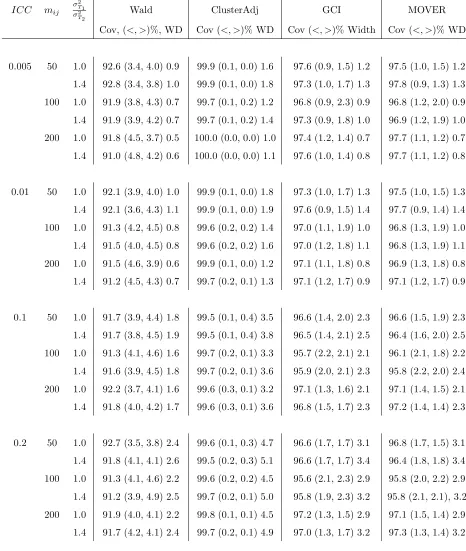
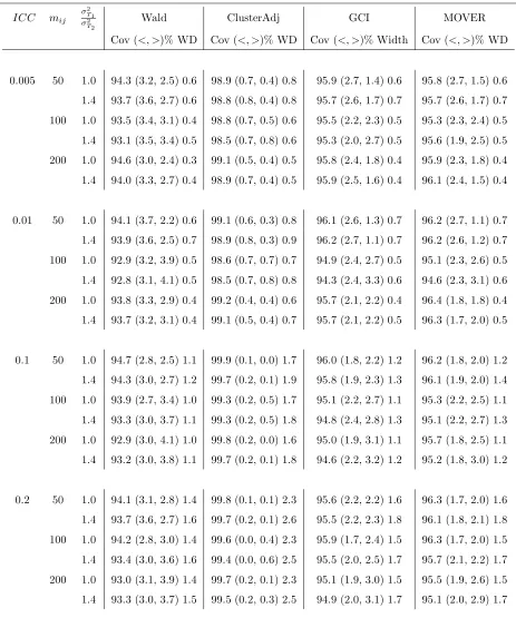
4.4 Empirical coverage (%), tail errors ((<, >)%), and median widths (WD) for the difference between two normal means when the number of clus-ters per arm equal 6 (control) and 6 (experimental), α = 0.05, imbal-ance parameter=0.8, and runs=1000 . . . 82 4.5 Empirical coverage (%), tail errors ((<, >)%), and median widths (WD)
for the difference between two normal means when the number of clus-ters per arm equal 12 (control) and 6 (experimental),α= 0.05, imbal-ance parameter=0.8, and runs=1000 . . . 83 4.6 Empirical coverage (%), tail errors ((<, >)%), and median widths (WD)
for the difference between two normal means when the number of clus-ters per arm equal 12 (control) and 12 (experimental), α = 0.05, im-balance parameter=0.8, and runs=1000 . . . 84 4.7 Empirical coverage (%), tail errors ((<, >)%), and median widths (WD)
for the difference between two normal means when the number of clus-ters per arm equal 24 (control) and 12 (experimental), α = 0.05, im-balance parameter=0.8, and runs=1000 . . . 85 4.8 Empirical coverage (%), tail errors ((<, >)%), and median widths (WD)
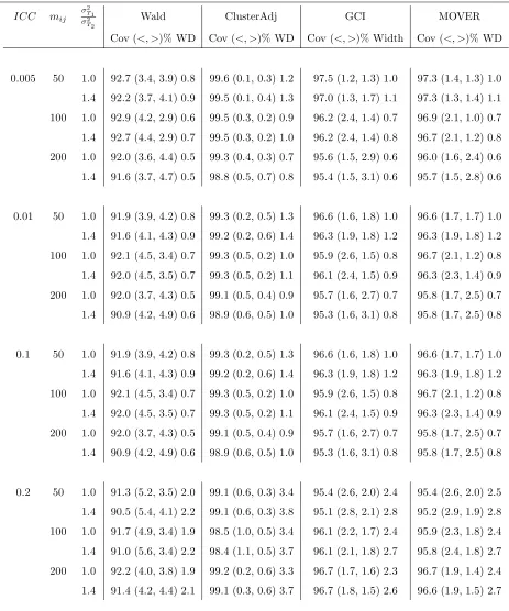
for the difference between two normal means when the number of clus-ters per arm equal 24 (control) and 24 (experimental), α = 0.05, im-balance parameter=0.8, and runs=1000 . . . 86 4.9 Empirical coverage (%), tail errors ((<, >)%), and median widths (WD)
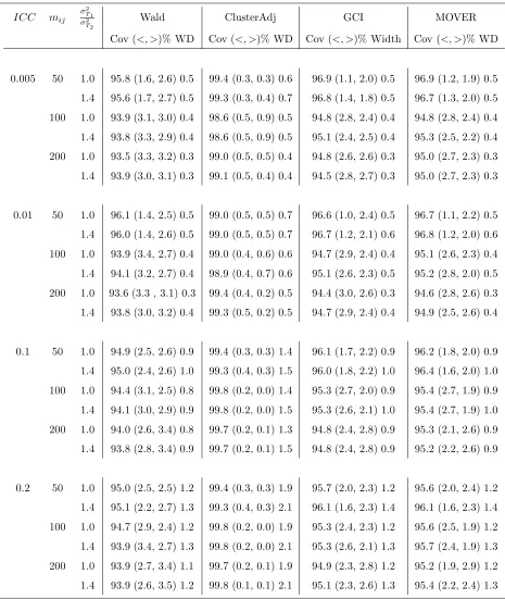
for the difference between two lognormal means when the number of clusters per arm equal 6 (control) and 6 (experimental), α = 0.05, imbalance parameter=0.8, and runs=1000 . . . 90 4.10 Empirical coverage (%), tail errors ((<, >)%), and median widths (WD)
for the difference between two lognormal means when the number of clusters per arm equal 12 (control) and 6 (experimental), α = 0.05, imbalance parameter=0.8, and runs=1000 . . . 91
imbalance parameter=0.8, and runs=1000 . . . 92 4.12 Empirical coverage (%), tail errors ((<, >)%), and median widths (WD)
for the difference between two lognormal means when the number of clusters per arm equal 24 (control) and 12 (experimental), α = 0.05, imbalance parameter=0.8, and runs=1000 . . . 93 4.13 Empirical coverage (%), tail errors ((<, >)%), and median widths (WD)
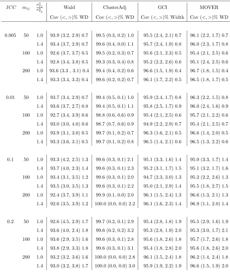
for the difference between two lognormal means when the number of clusters per arm equal 24 (control) and 24 (experimental), α = 0.05, imbalance parameter=0.8, and runs=1000 . . . 94 4.14 Empirical coverage (%), tail errors ((<, >)%), and median widths (WD)
for P(Y1 > Y2) = 0.5 when the number of clusters per arm equal 6
(con-trol) and 6 (experimental), α = 0.05, imbalance parameter=0.8, and runs=1000. . . 98 4.15 Empirical coverage (%), tail errors ((<, >)%), and median widths (WD)
for P(Y1 > Y2) = 0.5 when the number of clusters per arm equal 12
(control) and 6 (experimental), α = 0.05, imbalance parameter=0.8, and runs=1000. . . 99 4.16 Empirical coverage (%), tail errors ((<, >)%), and median widths (WD)
for P(Y1 > Y2) = 0.5 when the number of clusters per arm equal 12
(control) and 12 (experimental), α = 0.05, imbalance parameter=0.8, and runs=1000. . . 100 4.17 Empirical coverage (%), tail errors ((<, >)%), and median widths (WD)
for P(Y1 > Y2) = 0.5 when the number of clusters per arm equal 24
(control) and 12 (experimental), α = 0.05, imbalance parameter=0.8, and runs=1000. . . 101 4.18 Empirical coverage (%), tail errors ((<, >)%), and median widths (WD)
for P(Y1 > Y2) = 0.5 when the number of clusters per arm equal 24
(control) and 24 (experimental), α = 0.05, imbalance parameter=0.8, and runs=1000. . . 102 4.19 Empirical coverage (%), tail errors ((<, >)%), and median widths (WD)
for P(Y1 > Y2) = 0.9 when the number of clusters per arm equal 6
(con-trol) and 6 (experimental), α = 0.05, imbalance parameter=0.8, and runs=1000. . . 103 4.20 Empirical coverage (%), tail errors ((<, >)%), and median widths (WD)
for P(Y1 > Y2) = 0.9 when the number of clusters per arm equal 12
(control) and 6 (experimental), α = 0.05, imbalance parameter=0.8, and runs=1000. . . 104
and runs=1000. . . 105 4.22 Empirical coverage (%), tail errors ((<, >)%), and median widths (WD)
for P(Y1 > Y2) = 0.9 when the number of clusters per arm equal 24
(control) and 12 (experimental), α = 0.05, imbalance parameter=0.8, and runs=1000. . . 106 4.23 Empirical coverage (%), tail errors ((<, >)%), and median widths (WD)
for P(Y1 > Y2) = 0.9 when the number of clusters per arm equal 24
(control) and 24 (experimental), α = 0.05, imbalance parameter=0.8, and runs=1000. . . 107
5.1 Descriptive statistics for the computer clinical decision support system arm and usual care arm of the hypertension study . . . 123 5.2 The Wald-type confidence interval (Wald), cluster-adjusted confidence
interval, generalized confidence interval (GCI) and the MOVER for the difference between mean systolic blood pressure (mm Hg) in the treatment arm vs. the control arm. . . 124 5.3 Descriptive statistics for the critical pathway versus usual care for the
treatment of community acquired pneumonia. . . 126 5.4 The Wald-type confidence interval (Wald), generalized confidence
in-terval (GCI) and the MOVER for the difference between mean length of stay (in days) in the critical pathway arm and the usual care arm. 129 5.5 The Wald-type confidence interval (Wald), generalized confidence
in-terval (GCI) and the MOVER (MOVER) for the exceedance proba-bility of systolic blood pressure for the control arm vs. the treatment arm . . . 132
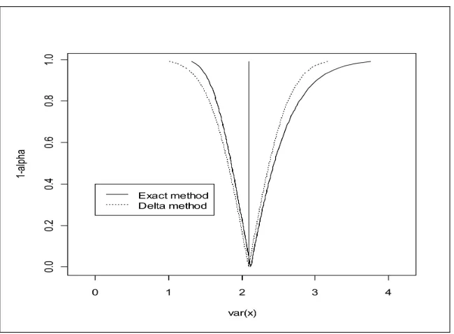
2.1 A confidence interval function of the delta method and the exact pro-cedure for the normal variance (σ2 = 2, s2 = 2.1, n= 100) . . . . 38
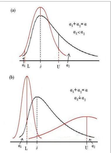
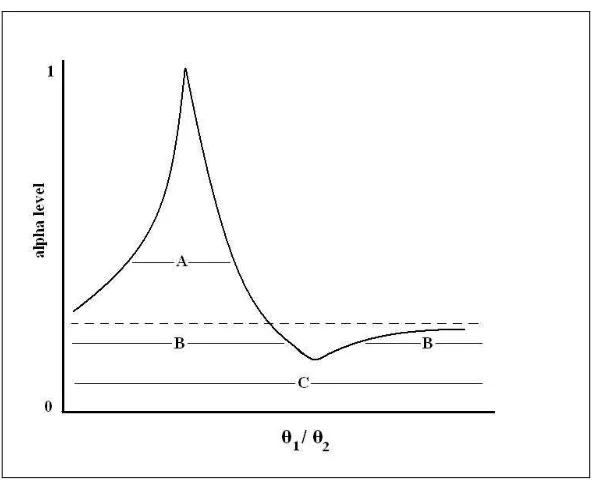
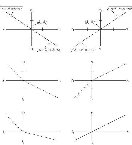
2.2 a) A symmetric confidence interval (L, U) for a summary measure (ˆθ) of data following a skewed distribution using traditional methods. b) An asymmetric confidence interval (L, U) for a summary measure (ˆθ) of data following a skewed distribution, by application of the MOVER. 41 2.3 Confidence interval curve for a ratio of two parameters . . . 47 2.4 The flexibility of the MOVER for differences and sums as shown using
margins of errors and the Pythagorean theorem . . . 50
5.1 Q-Q plots of SBP by practice (7 clusters) in the usual care arm . . . 121 5.2 Q-Q plots of SBP by practice (10 clusters) in the clinical decision
sup-port system with cardiovascular risk chart arm . . . 122 5.3 Q-Q plots of log length of stay (10 clusters) in the usual care arm . . 127 5.4 Q-Q plots of log length of stay (9 clusters) in the critical pathway arm 128
Chapter 1
INTRODUCTION
1.1 Randomized controlled trials
A randomized controlled trial is an experiment that randomly assigns units to different
intervention groups, usually a control group and an experimental group. Successful
randomization can prevent selection bias and balance intervention groups for both
known and unknown factors associated with the outcome of interest such that the
arms of the trial will differ only according to the intended difference being tested
(Julious and Zariffa, 2002). Thus, a well conducted randomized controlled trial is
usually considered as the gold standard for evaluating health care interventions.
Con-sequently, many systematic reviews of the effects of health care interventions, such
as those of the Cochrane Collaboration, are carried out primarily using data from
randomized controlled trials (Clarke et al., 1999, section 13.1.3).
1.2 Cluster randomization trials
Cluster randomization trials are a special case of randomized controlled trials where
intact social units, rather than individuals, are randomly allocated to the arms of the
trial. These social units are commonly termed “clusters”.
Cluster randomization trials have a number of interesting properties. As with
in-dividually randomized trials, on average, cluster randomization balances comparative
groups according to known and unknown factors associated with the outcome of
inter-est (Donner and Klar, 2000, page 11). Therefore, it is used to eliminate confounding
Cluster sizes are diverse, ranging from as few as one or two individuals to hundreds
of thousands. Examples of clusters include families, schools, work sites, physician
practices, and entire communities. Another example is given by Daltroy et al.(2007), who randomized ferry boats on which entertainment troupes delivered an educational
intervention about how to prevent Lyme disease by avoiding contact with ticks.
A distinctive property of cluster randomization trials is that observations within
each cluster may be correlated. If inferences are made at the cluster level, then this is
not an issue. However, if inferences at the individual level are of interest, clustering
may lead to reduced efficiency and a potentially complicated analysis as compared
to individual level randomization. Consequently, the effects of clustering must be
accounted for in the design and the analysis of the study if the unit of inference (e.g.
the individual) differs from the unit of random allocation (e.g. the cluster).
Due to the potential loss in efficiency and the increased complexity of the analysis
of cluster randomization trials when the unit of randomization differs from the unit of
inference, justification for adopting the clustered design is necessary. Several common
reasons warrant the use of a cluster randomization trial. First, interventions may
only be delivered at the cluster level. This strategy was adopted by Williamson
et al. (2007) who compared the effects of an environmental intervention (including changes to the cafeteria menu) to those of an active control for preventing weight
gain in children. Since the change to the cafeteria menu is designed to be delivered
to an entire school, it would not be feasible to randomize individuals to receive this
intervention. Randomization must necessarily be at the cluster level, the school.
Second, given that individuals in the same cluster are likely to interact,
randomiz-ing clusters to intervention groups commonly reduces contamination across the arms
of a study. For example, Sankaranarayanan et al.(2007) evaluated the effect of visual screening as compared to usual care on cervical cancer incidence and mortality in
India by randomizing villages to reduce contamination within each village.
investi-gators, improve logsitic convenience, or decrease the cost of the study. For instance,
Trevinoet al. (2004) randomized schools to receive either an educational intervention or usual care for the purpose of decreasing capillary glucose levels in an attempt to
control diabetes mellitus. A clustered design was chosen because programs which
include social support and peer pressure tend to improve compliance (Perri et al., 1988).
Finally, if the objective of a study is to obtain the total effect of an intervention,
a clustered design may be employed. With certain interventions it may be feasible
to randomize at either the individual or cluster level, but if the question of interest
lies at the cluster level, the unit of randomization must necessarily be the cluster.
A common example arises from studies of infectious disease, where both direct and
indirect effects are of interest (Hayes and Moulton, 2009, Chapter 3). Direct effects
of an intervention such as an immunization may be captured using an individually
randomized trial. However, indirect effects include the effects of an intervention which
is administered to others, such as herd immunity. Unfortunately, this type of effect
cannot be measured in a trial which randomizes individuals. A cluster randomization
trial on the other hand would allow the measure of direct, indirect, and total (the
combination of direct and indirect) effects of the intervention. Melese et al. (2008) were interested in the effect of biannual antibiotic treatment on infectious trachoma
as compared to an annual treatment. The total effect of antibiotic treatment on the
population was of interest. This was measured by the comparison of village prevalence
of occular chlamydial infection, therefore villages were randomized to each arm.
Oftentimes a cluster randomization trial design is used for multiple reasons. For
example, a recent cluster randomization trial (Pandey et al., 2007) randomized dis-tricts (each containing 5 village clusters) in the Uttar Pradesh state in India to
inves-tigate the impact on health and social services delivered by the villages by informing
resource-poor rural populations about entitled services. The advantage of
obtained from a single state which determined both health and educational services.
Furthermore, randomization by cluster was adopted to lower the level of
contamina-tion, as travel between intervention and control villages would have been difficult.
When there are acceptable justifications for clustering, there are a number of trial
designs to choose from. The most commonly used clustered designs are the completely
randomized design, the stratified design, and the matched-pair design.
In a completely randomized cluster trial all of the clusters involved in the study are
randomly allocated to the arms of the trial without the statifying or mathing baseline
characteristics. For instance, this design was used by Vizcaino et al. (2008), where no stratification was used to randomize twenty schools to receive either a physical
activity program or usual care to prevent childhood obesity. In this case, random
allocation was performed using a computer generated procedure.
An implication of randomizing clusters, however, is that only a small number of
clusters may be involved in the study, especially when the cluster sizes are large.
As such, randomization may not ensure balance of cluster level confounders between
arms. In such cases, stratification or matching may be useful to increase balance
between the arms of a trial. For the stratified and matched-pair designs, the clusters
in each stratum are assigned according to baseline characteristics or similarities
be-tween clusters such that these characteristics are potentially related to the outcome.
Examples of common matching characteristics include cluster size and geographical
location.
A stratified design assigns multiple clusters to different interventions within each
stratum. This design was adopted by Naylor et al. (2006) who studied the effect of a physical-activity action plan in schools on physical activity level. With so few
clusters, cluster size and geographic location may not have been balanced between
trial arms, so the ten schools were first stratified by these variables, then the clusters
within each stratum were randomly assigned to the two study arms.
two clusters within a stratum, such that there is a very tight balance of baseline
characteristics associated with the outcome between these two clusters. Each cluster
in a pair is then randomly allocated to a different arm. As an example, Flanneryet al.
(2003) matched eight schools based on geographic proximity, the percentage of ethnic
students, the percentage of students eligible for free or reduced-price lunch, and the
percentage of students in English as a Second Language classes. These clusters were
randomized to determine the effect of an immediate social peace building intervention
on violence prevention, as compared to a delayed intervention. It is important to
recognize that the lack of replication of clusters to each arm within each stratum
complicates the ability of quantifying the similarity of individuals within each cluster
as compared to between clusters, because the variation of responses between clusters
is confounded with the effect of intervention. Thus, data from such a design is usually
analyzed at the cluster level (Klar and Donner, 1997).
1.3 Notation
Correlated continuous outcomes commonly arise from cluster randomization trials,
where these responses may often be approximated with the normal distribution. To
allow for a more detailed discussion about useful effect measures, we now digress to
introduce some notation by starting with an assumption that data from each arm
of the trials is assumed to follow a one-way random effects model. This assumption
allows two levels of variance - one at the individual level and one at the cluster level.
Furthermore, attention is limited to a completely randomized trial design for the sake
of simplicity.
Suppose ki clusters are randomized to intervention i (i = 1,2). Let mij denote
the jth cluster size (j = 1, ...k
i) of arm i. Now let
Yijl =µi+Aij +Eijl, (1.1)
arm i, µi is the population mean of arm i, and Aij ∼ N(0, σ2Ai) is independent of
Eijl ∼N(0, σE2i).
Continuing with the case of two arms, the three parameters in each arm include
the overall mean (µi), the between-group (or between-cluster) variance component
(σ2
Ai), and the within-group (within-cluster) variance component (σ 2
Ei). Observations
can then be used to estimate these three parameters. Attention is limited to Analysis
of Variance estimators of variance components, as recommended for low to moderate
values of the intraclass correlation coefficient (ICC) (see Section 1.4.2) (Donner and
Koval, 1980). This thesis focuses on small to moderate values of the ICC, as discussed
in Chapter 4.
The overall mean of arm i, µi, may be estimated by
¯¯
Yi =Mi−1
X
j
X
l
Yijl,
where Mi = Pjmij denotes the total number of individuals in arm i. The
cluster-specific mean may be estimated by
¯
Yij =m−ij1
X
l
Yijl.
To estimate the variance components, denote
MSCi =
SSCi
ki−1
and
MSWi =
SSWi
Mi−ki
as the mean squared errors between- and within-clusters, respectively, where
SSCi =
X
j
mij
¯ Yij −Y¯¯i
2
and
SSWi =
X
j
X
l
Yijl−Y¯ij
2
.
The between-cluster variance component may be estimated by
SA2i = MSCi−MSWi moi
,
where
moi =
Mi−Pjm2ij/Mi
ki−1
,
and the within-cluster variance component by
SE2i = MSWi.
An estimate of the total variance in arm i is then given by S2 Ti =S
2 Ai +S
2 Ei.
When all cluster sizes are equal (or balanced), the estimated parameters of each
arm (assumed to follow a one-way random effects model) of a cluster randomization
trial follow familiar distributions. That is,
¯¯
Yi ∼ N
µi,
σ2 Ai+σ
2 Ei/mi
ki
(Donner and Klar, 2000, page 8),
SSCi
σ2
Ei+miσ 2 Ai
∼ χ2ki−1, and
SSWi
σ2 Ei
∼ χ2
Mi−ki (Graybill, 1976, page 609). (1.3)
These properties may be used to construct confidence intervals for the overall mean
and variance components of the model.
However cluster sizes are rarely balanced in practice. Although SSWi/σE2i ∼
χ2
Mi−ki approximately holds for the unbalanced design, SSCi/(σ 2
Ei+miσ 2
Ai) no longer
follows a chi-squared distribution and the variance of ¯¯Yi must be adjusted (Burdick
et al., 2006). Thomas and Hultquist (1978) proposed an unweighted mean squared error which may be used in the unbalanced design,
SU i2 = nHi P
j( ¯Yij −Y¯¯i)2
ki−1
, (1.4)
where
E(SU i2 ) = σE2i+nHiσA2i,
nHi =
ki
P
is the harmonic mean of the cluster sizes, and
(ki−1)SU i2
σ2
Ei +nHiσ 2 Ai
∼χ2ki−1.
The variance estimate of the estimated overall mean, ¯¯Yi, is then given bySU i2 /(kinHi)
(for i= 1,2).
1.4 Brief summary of methods for cluster randomization trials with continuous data
The primary purpose of conducting a cluster randomization trial is to make
compar-isons between arms. The first step of meeting such an objective is to obtain a useful
summary statistic that answers the primary question of interest of the study. The
primary question of interest informs whether the analysis will be performed at the
cluster level or at the individual level. We start with cluster level analysis as the
methods are simpler.
Cluster-level analyses
Although randomization in a cluster randomization trial occurs at the cluster level,
investigators usually have a choice between cluster-level or individual-level analyses.
Cluster-level analysis begins with creating cluster-specific summary statistics, followed
by the application of standard statistical methods which are approximately valid.
Each cluster level summary measure is then treated as a single observation, and
clusters are independent.
Cluster-level analyses are appropriate when the primary question of interest is
directed not to the individual, but to the randomized unit. For example, Lenhart
et al. (2008) were interested in determining the effect of insecticide treated bednets on the transmission of vector-borne diseases and dengue by mosquitos in Haiti. The
with them. In this study, 9 pairs of sectors containing a total of 1017 houses were
randomized to either insecticide treated bednets or bednets which were not treated
(usual care). The outcome of primary interest in this case was the number of trap
containers with mosquitos with immature stages of disease per 100 households. A
paired t-test was used to obtain inferences on this cluster-level outcome, where it
was found that insecticide treated bednets had an immediate positive effect on vector
diseases and dengue transmission.
As standard statistical methods may be used to analyze data at the cluster level,
many valid and efficient procedures already exist. This thesis therefore focuses on
analysis procedures at the individual level. Thus, unless otherwise stated, any mention
of statistical analyses refers to individual level methods rather than those at the cluster
level.
Individual level analyses
Although randomization occurs at the cluster level, inferences at the individual level
are commonly of interest. For example, in a prenatal care study, Villar et al. (1998) evaluated a new antenatal care program by comparison to standard care through a
cluster randomization trial, where the program’s effects on birth weight was of primary
interest. As another example, Christianet al. (2003) randomized 426 communities to five trial arms to determine the effect of micronutrient supplements on birth weight,
where comparisons were made using the differences in average birth weights between
each treatment arm and the control. To obtain inferences on this difference at the
individual level, both between cluster and within cluster variance components must
be accounted for.
Clusters in a cluster randomization trial may be assumed to be independent,
however the individuals within each cluster may not. Two individuals in the same
cluster are likely to be more similar than two individuals from different clusters (Hayes
clustered design: the variation within clusters (σ2
E) and the variation between clusters
(σ2
A), where the total variation equals σ2T = σ2A+σE2. Clustering occurs when the
variation between clusters is non-zero. Therefore, these variance components may be
used to quantify the similarity of individuals within the same cluster.
Two indices have been used to quantify the similarity of responses within clusters
rather than between. The first is the intraclass correlation coefficient (ICC) (Donner
et al., 1981), interpreted as the standard Pearson correlation coefficient between two responses in the same cluster. It is given by the ratio of the between cluster variance
component to the total variance (ρ =σ2
A/σT2). When the responses of individuals in
the same cluster are no more similar than those of other clusters, the between cluster
variation and consequently the ICC both equal zero. At the other extreme, when all
of the responses of individuals in the same cluster are identical, the within cluster
variance component equals zero, and the ICC equals one. The majority of the time,
the ICC falls between these two extremes. In a review by Eldridge et al. (2004), the median ICC value for cluster sizes of around 30 was 0.04, with an interquartile
range of −0.02 to 0.21. Larger clusters such as communities typically have smaller
ICC values of 0.002 to 0.012 (Hannan et al., 1994). Note that negative ICC values are possible, but improbable, typically occurring when individuals within the same
cluster are less similar to one another than to individuals in other clusters (Hayes and
Moulton, 2009, page 17). Due to their rare occurrence (Donner and Klar, 2000, page
11), negative ICC values will not be investigated further.
The second index used to account for dependent responses in a cluster is the
coef-ficient of variation between clusters (CVA =σA/µ) (Hayes and Moulton, 2009, page
16). As the similarity in responses of two individuals in the same cluster with respect
to other clusters increases, the difference in the responses between clusters will also
increase. That is, the variance of the cluster-specific means will increase. The
be-tween cluster coefficient of variation measures the spread of the cluster-specific means
individu-als in the same cluster are no more similar than the responses of two individuindividu-als in
different clusters, then σ2
A = 0 and CVA = 0. However, when the responses of two
individuals in the same cluster are more similar than the responses of two individuals
in different clusters, thenσ2
A>0 and CVA>0 (assuming that µ >0). Shoukri et al.
(2008) and Quan and Shih (1996) give a description of the within-cluster coefficient
of variation (CVE = σE/µ) as a measure of reproducibility. However, this measure
(CVE) is not as relevant to quantifying the effect of clustering as CVA, because it
gives no information about existing differences between clusters.
The common element in both the ICC and the between-cluster coefficient of
vari-ation is the between-cluster variance component, σ2A. These statistics may further be
used to quantify the effect of clustering for analysis at the individual level.
The effect of clustering on data analysis may be quantified by the design effect
(Donner and Klar, 2000, page 8). The design effect is interpreted as the ratio of
the variance of the estimated effect measure for cluster sampling to that of random
sampling, and is given as (Hayes and Moulton, 2009, page 21)
deff = 1 + (m−1)ρ (1.5)
= 1 + (m−1)σ
2 A
σ2 T
= 1 + (m−1)σ
2 A
σ2 T
µ2 µ2
= 1 + (m−1)CVA
µ2
σ2 T
, (1.6)
where m is the size of the clusters.
Once the effect of clustering is quantified, there are a variety of analysis procedures
to choose from. The choice of analysis procedure depends on the question of interest
Current methods for a difference between two normal means
The responses from a cluster randomization trial may often be approximated with
the normal distribution. For instance, body weight, height, body temperature, blood
pressure, or summary scores from standardized questionnaires frequently follow
nor-mal distributions. For example, Kinra et al. (2008) randomized villages in India to investigate the effect of protein-calorie supplementation and public health
pro-grammes on cardiovascular risk. Outcome measures in this study included height and
blood pressure, and were assumed to be normally distributed. As another example,
Montgomery et al. (2000) randomized twenty-seven general practices to investigate the effect of a computer based clinical decision support system and a risk chart on
blood pressure, an outcome which may be assumed to follow a normal distribution.
This data is used in Chapter 5 as an illustration of the methods investigated in this
thesis.
When sample means and their differences are assumed to follow normal
distribu-tions, confidence intervals or hypothesis tests for a difference between means or the
equality of means may be used to draw conclusions from a cluster randomization trial.
Because they encompass hypothesis testing, confidence intervals are preferred. This
claim is detailed in Chapter 2.
A method proposed by Donner and Klar (1993) is to use the design effect
(Equa-tion (1.5)) to adjust the variance of the difference for clustering. The inflated variance
is then plugged into the usual t-interval, setting degrees of freedom to the number
of clusters minus two. This procedure uses a pooled estimate of the standard error,
thereby assuming equal variances (homoscedasticity) in the two arms being
com-pared. As in the case of individually randomized designs, variance homogeneity can
be assumed in hypothesis testing when the null hypothesis is true, but not in the
con-struction of confidence intervals (Wang and Chow, 2002). Donner and Klar (1993)
a common design effect under the null hypothesis.
To avoid the homoscedasticity assumption of many statistical inference procedures,
the variance in each arm of a cluster randomization trial may be estimated separately.
The usual variance estimate which ignores clustering is biased when ICC>0,
under-estimating the total variance (White and Thomas, 2005). Instead, the total variance
of the overall mean in each arm of a clustered trial is given by (Donner and Klar,
2000, page 8)
var( ¯Yi) =
σ2
A+σE2/m
k ,
where k is the number of clusters of size m. This cluster-adjusted variance may be
estimated using the unweighted mean squared error (Thomas and Hultquist, 1978)
for variable cluster sizes. El-Bassiouni and Abdelhafez (2000) showed that using the
unweighted mean squared error to construct a confidence interval for a single normal
mean from a one-way random effects model maintains the desired coverage, although
tends to be wide when the ICC is less than 0.2. This confidence interval method may
be applied here, because the observations in each arm of a cluster randomization trial
may be assumed to follow a one-way random effects model.
Another approach to the above closed-form procedures is the generalized
confi-dence interval method (Weerahandi, 1993). Generalized conficonfi-dence intervals are based
on the simulation of a known generalized pivotal quantity that possess the following
two properties:
(i) its probability distribution is not dependent on any unknown parameters and
(ii) the observed value is not dependent on any unknown nuisance parameters.
Property (i) of the generalized pivotal quantity ensures that the confidence region
may be found without the knowledge of unknown parameter values. This property
function of observations and unknown parameters, but whose distribution does not
depend on any unknown parameters. Property (ii) of the generalized pivotal quantity,
which is not found in the usual definition of pivotal quantities, further ensures that
the confidence region may be obtained with only the use of the observed data.
To construct a generalized confidence interval, the generalized pivotal quantity
is simulated a large number of times and the limits are set to the α/2 and 1−α/2
quantiles. However, certain drawbacks of generalized confidence intervals arise as a
consequence of property (ii): aside from having to know the generalized pivotal
statis-tic in advance, generalized confidence intervals do not have a closed form, because
the observed pivotal is based on simulation. Consequently, two generalized confidence
intervals of the same confidence coefficient for the same dataset may differ. This may
make a difference particularly in cases where there is a composite parameter of
inter-est.
More complex methods of analysis include mixed regression models (Harville, 1977;
Harville and Jeske, 1992) and generalized estimating equations with an exchangeable
correlation matrix (Liang and Zeger, 1996). When there are a small number of clusters
involved in a trial, there may be chance imbalance of covariates that are predictive of
the outcome. These methods have the ability to adjust for unbalanced covariates in
different trial arms. Unfortunately, the methods may be invalid when there are fewer
than fifteen clusters per arm (Hayes and Moulton, 2009, Chapter 11), precisely when
chance imbalance of covariates may occur, although improvements have been
sug-gested (Skene and Kenward, 2010). Additionally, regression methods and generalized
estimating equations as applied to cluster randomization trials sacrifice the desired
simplicity of many of the confidence interval procedures discussed thus far.
Covari-ate adjustment procedures will therefore be exempt from this thesis. Extensions for
1.5 Alternative effect measures in cluster randomization trials
The standardized mean difference
Some outcomes are not as easily interpreted on the raw scale as outcomes such as
height, weight, or blood pressure which have a natural comparison using a difference.
For example, quality of life scores are a subjective assignment of values based on a
combination of features. Other subjective ratings may also have this problem. In
such cases, investigators often compare two groups using Cohen’s effect size (Cohen,
1988), defined by the difference in the magnitudes of treatment effects in units of
standard deviation. For instance, Jordhoyet al.(2001) randomized community health districts and used the effect size as the summary measure to assess the impact of
comprehensive palliative care compared with conventional care on the quality of life
of cancer patients. Also, Bernstein et al. (2005) randomized schools to three arms to compare effectiveness of school-based interventions for anxious children. The primary
outcome was the change in composite clinician severity rating from baseline to
post-treatment, where the effect size was used as the summary measure when comparing
the arms of the trial. Also note that the effect size is often used to summarize results
in a meta-analysis. For example, in the meta-analysis by Brunoni et al. (2009) the effect size was used to show that placebo responses of major depressive disorders are
large regardless of the intervention of the study.
The choice of the effect size expression is more complicated in cluster
randomiza-tion trials than in individually randomized trials. In an individually randomized trial,
the effect size is set to the difference between means divided by the standard
devi-ation. This standard deviation may be set to the pooled sample standard deviation
(Hedges and Olkin, 1985), with an interpretation of the difference between means of
two arms in terms of the extent to which individual responses vary. Alternatively,
the denominator may be set to the control group standard deviation, leading to a
which control group individuals vary amongst one another. However, in cluster
ran-domization trials which have two levels of variation, there are even more possibilities
for the denominator. Hedges (2007b) discusses three possibilities, each depending on the inference of interest to the researcher. These possibilities include setting the
denominator to a function of the within cluster variance component, the between
cluster variance component, or the total variance. Consequently, each would have a
slightly different interpretation, potentially complicating the summary of results in
meta-analyses which often include both cluster randomization trials and individually
randomized trials.
Another issue lies with the direct interpretation of the effect size. Cohen (1988)
defined “small”, “medium”, and “large” effect sizes as 0.2, 0.5, and 0.8, respectively.
However, this interpretation is meant for application to the behavioral sciences, not
necessarily as a generalization to all disciplines. Furthermore, the interpretation in
units of standard deviations has more of a statistical meaning rather than a clinical
meaning, potentially complicating results to a clinician. Also, although this
mea-sure has gained popularity in the behavioral and social sciences, there is no clear
interpretation to the measure in a probabilistic sense.
Using the standard normal cumulative distribution function, it can be shown that
the interpretation of the effect size is a function of the probability that the observation
(Y1) of a randomly selected individual from one arm of the trial is larger than the
mean of another arm (µ2). That is, assuming µ2 > µ1 and homoscedasticity for
simplicity,
P(Y1 > µ2) = P(Y1−µ1 > µ2−µ1)
= P
Y1 −µ1 √
σ2 >
µ2−µ1 √
σ2
= P
Z > µ2√−µ1
σ2
= Φ
µ1 −µ2 √
σ2
where σ2 is the pooled variance. Note that if µ
1 > µ2 then the effect measure would
be Φµ√2−µ1
σ2
. However, there are two clear concerns with this interpretation. First,
the true mean (µ2) is rarely known in practice. Second, it is illogical to interpret
study results by comparing a randomly selected individual in one arm to the mean
of the observations from another arm. This comparison does not generally answer
typical questions which motivate the conduct of cluster randomization trials.
It would be more logical to find the probability that a randomly selected individual
in one arm has a larger outcome than a randomly selected individual in another arm,
P(Y1 > Y2). For example, in a medical context comparing the responses of two
treatments, where Y2 represents the response under treatment 1 and Y2 represents
the response under treatment 2, P(Y1 > Y2) = 0.7 makes more sense to a clinician
and a patient than does (µ1−µ2)/σ= 1. Let us refer to P(Y1 > Y2) as the exceedance
probability.
In the past, the exceedance probability has been described as intuitive and simple
(McGraw and Wong, 1992; Grissom, 1994; Kraemeret al., 2003) and has shown wide application in the literature. For instance, its application may be found in reliability
measurements (Church and Harris, 1970) and clinical equivalence trials (Haucket al., 2000). It is also closely related to the area under the receiver operator characteristic
curve and to non-parametric statistics (Acion et al., 2006). It is its application to cluster randomization trials which is of interest here.
LetY1 ∼N(µ1, σT21) and Y2 ∼N(µ2, σ
2
T2) represent observations from two arms of
a cluster randomization trial, whereσ2 Ti =σ
2 Ai+σ
2
then be manipulated to uncover the effect measure which is of applicable interest,
P(Y1 > Y2) = P(Y1 −Y2 >0)
= P(Y1 −Y2−(µ1−µ2)>−(µ1−µ2))
= P
Y1 −Y2−(µ1−µ2)
q σ2
T1 +σ
2 T2
> q−(µ1−µ2) σ2
T1 +σ
2 T2 (1.7) = P
Z > −(µ1−µ2)
q σ2
T1 +σ
2 T2 = Φ
(µ1−µ2)
q σ2
T1 +σ
2 T2
.
The effect measure of interest is thus a monotone function of the standardized mean
difference,
δ = qµ1 −µ2 σ2
T1 +σ
2 T2
. (1.8)
Although the term ‘standardized mean difference’ is often used interchangeably with
‘Cohen’s effect size’, here it will refer to δ. Confidence intervals for P(Y1 > Y2) may
then be obtained from confidence intervals for δ using the transformation principle
(see Section 2.3.2).
In addition to having a logical interpretation, this measure is capable of capturing
all of the effects of the treatment as compared to the control. A difference in means
is clearly useful when comparing overall results. However, the variability in each arm
of the cluster randomization trial reflects the consistency in response. Since δ is a
function of the means and variances, it takes into account both the magnitude and
consistency of responses.
Once the exceedance probability is estimated, it is important to obtain inferences
on this measure. Obtaining inferences onδis more complicated in cluster
estimates of the standardized mean difference follows the non-central t-distribution
with non-centrality parameter µ1 −µ2 (Owen et al., 1964). However, as a result of
the two levels of variation present in clustered designs, this relationship does not hold
(Thomas and Hultquist, 1978). The estimates of δ and P(Y1 > Y2) do not follow
exact distributions, and therefore exact confidence intervals may not be obtained.
Confidence interval procedures forδare scarce because the parameter is a function
of the normal mean (µ), the between-cluster variance component (σ2
Ai) and the
within-cluster variance component (σ2
Ei). One option is to apply the multivariate delta
method to obtain an expression for the variance of the estimate ofδ. Slutsky’s theorem
(Casella and Berger, 2002, page 239-240) states that
If Xn→X in distribution and Yn →a, a constant, in probability, then
i) YnXn→aX in distribution and
ii) Xn+Yn→X+a in distribution.
Using Slutsky’s theorem, the estimated variance at the point estimate may then be
plugged into Wald type confidence intervals which are constructed by inverting the
Wald test (Wald, 1941). That is, the limits are set to the point estimate plus or minus
some multiple of this estimated standard error. By using this plug-in principle, the
estimated variance used for the upper limit is forced to equal the estimated variance
used when constructing the lower limit, thus yielding symmetric limits around the
point estimate. In fact, any Wald-type confidence interval procedure which utilizes
this plug-in principle will have this restriction. However, as in individually randomized
trials, the estimate ˆδ may have a skewed sampling distribution in cluster
randomiza-tion trials. Therefore, one limit of a symmetric confidence interval may fail to exclude
all extreme values while the other limit may exclude too many values. Confidence
interval procedures which take into account the shape of the distribution are therefore
desirable.
The Fieller method (Fieller, 1954) is not restricted to symmetry and may be used
assumes that the sampling distribution of both the numerator and the denominator
are normal. Although the estimated numerator of the standardized mean difference
may be approximately normal, the denominator is a function of estimated variance
components. The unweighted mean squared error (Equation (1.4)) may be used
to approximate the denominator, and Thomas and Hultquist (1978) show that this
statistic is approximately proportional to the chi-squared distribution. Thus, the
denominator of the standardized mean difference is typically skewed in distribution.
Therefore, the Fieller method would also fail to capture the underlying distribution
of the effect measure.
Alternatively, generalized confidence intervals may be constructed for the
stan-dardized mean difference, and thus for P(Y1 > Y2), when the data in each arm follow
a one-way random effects model. Recall from Section 1.4.3 that this method requires
the existence of a generalized pivotal statistic. Using the results of Thomas and
Hultquist (1978), Krishnamoorthy et al. (2007) provide generalized pivotal statistics for the normal mean, the between-group variance component, and the within-group
variance component when data follow a one-way random effects model,
Gµ = ¯¯Y +
Z q
χ2 k−1
r SSC
k , (1.9)
Gσ2
A =
SSC χ2
k−1
−n˜χSSW2 M−k
+
, (1.10)
Gσ2
E =
SSW χ2
M−k
, (1.11)
where Z ∼ N(0,1), χ2
df is a random variable from the chi-squared distribution with
df degrees of freedom, SSC is the sum of squares between groups, SSW is the sum of
squares within groups, (x)+ = max{0, x}+, and ˜n = (1/k)Pkj mj. Thus, Equations
(1.9) to (1.11) may be obtained by plugging in both summary statistics of the data
as well as simulated standard normal and chi-squared random variables. These three
generalized pivotal statistics may then be used to obtain a generalized pivotal statistic
because an attractive feature of the generalized confidence interval procedure is that
the generalized pivotal statistic of a function of parameters is simply that function
applied to the generalized pivotal statistics of those parameters. Thus, as long as the
generalized pivotal quantity of the components of a particular parameter of interest
are known, the generalized pivotal quantity of the parameter may be found.
As the standardized mean difference is given by Equation (1.8), the generalized
pivotal quantity of this statistic may be expressed as
Gδ =
Gµ1 −Gµ2
q Gσ2
A1 +Gσ2E1 +GσA22 +Gσ2E2
.
To obtain generalized confidence intervals (Lδ, Uδ), an algorithm similar to that found
in Krishnamoorthy et al. (2007) may be used with Gδ. Generalized confidence
inter-vals for P(Y1 > Y2) are then given by (Φ(Lδ),Φ(Uδ)).
Generalized confidence intervals have not previously been applied to the
standard-ized mean difference or to P(Y1 > Y2) when data arise from a cluster randomization
trial. Theoretically, their application would not result in symmetric limits around a
parameter with a skewed sampling distribution like those of the Wald interval.
How-ever, recall that their application would not result in closed form intervals. A closed
form procedure is preferable.
The difference between two lognormal means
In addition to the normal distribution, data found in practice may commonly be
ap-proximated by the lognormal distribution. For instance, when a variable is bounded
with a concentration of data falling near the lower bound, then the data may be
skewed, potentially following a lognormal distribution. Also, according to the
mul-tiplicative central limit theorem, the multiple of a large number of independent and
positive random variables, each with a finite mean and variance, will approximately
commonly follow lognormal distributions in practice include hospital wait times and
cost data (Thompson and Barber, 2000). Panellaet al.(2007) randomized 14 hospitals to either treatment according to a clinical pathway or usual care, where non-normal
outcomes of interest included length of hospital stay and overall cost. Also, Marrie
et al.(2000) investigated the efficiency of a critical pathway, randomizing 19 hospitals to either continued conventional management or to implement the critical pathway.
One of the outcomes was the length of hospital stay which may be approximated by
the lognormal distribution, as we shall see in Chapter 5 where we used this data as
an illustration for the methods investigated in this thesis. Similar to outcomes which
may follow a normal distribution, two arms of a cluster randomization trial may
nat-urally be compared using a difference of means when outcomes are approximately
lognormal.
Obtaining inferences on a single lognormal mean has been a challenge when data
follow a one-way random effects model on the log scale (Briggs et al., 2005). This is because the lognormal mean is a function of three parameters: the normal mean
(µ), the between-group (or between-cluster in an arm of a cluster randomization
trial) variance component (σ2
A), and the within-group (or within-cluster) variance
component (σ2
E). Existing inference procedures are limited in scope, requiring not
only the assumption of homoscedasticity, but symmetric confidence intervals when
the lognormal distribution is skewed in shape. An example of this arises when the
multivariate delta method is used to estimate the variance of the lognormal mean at
the point estimate, which is then plugged into the Wald-type intervals using Slutsky’s
theorem. Again, the shape of the confidence interval should reflect the shape of the
distribution, thereby ensuring that only the extreme values are excluded.
Two types of procedures which are not restricted to symmetry are bootstrap
pro-cedures and generalized confidence intervals. Bootstrap confidence intervals have
become popular since they were first introduced by Efron (1979), and their use is
and Efron, 1996). However, the performance of the bootstrap has not been ideal for
the lognormal mean. Recall that the lognormal mean is a function of the normal
mean and variance. DiCiccio and Efron (1996) and Schenker (1985) have shown that
the percentile method and the bias-corrected bootstrap procedures for the normal
variance have low coverage when sample sizes are small to moderate. These results
seem to be consistent throughout the literature. More recently, Dinh and Zhou (2006)
and Zou and Donner (2008) have shown that bootstrap confidence interval procedures
have low coverage for the lognormal mean when data on the log scale follow a fixed
effects model. Also, Flynn and Peters (2004) used Monte Carlo simulations to show
that the bias-corrected and accelerated bootstrap procedure lead to confidence
inter-vals with low coverage for a difference between mean costs in cluster randomization
trials, where cost data are normally and lognormally distributed.
The poor performance of the bootstrap in these cases stems from the fact that the
bootstrap procedure requires the existence of a transformation which can make the
sampling distribution of the statistic of interest both normal and pivotal (Schenker,
1985). Such a transformation does not seem to exist for the normal variance. For
instance, the log transformation makes it pivotal but not normal, and the cubic root
transformation makes it normal but not pivotal (Kendall and Stuart, 1977, page 371).
Alternatively, generalized confidence intervals may be constructed for a difference
between two lognormal means when the data are assumed to follow a one-way random
effects model on the log scale. The required pivotal statistic may be constructed using
Equations (1.9), (1.10), and (1.11). This statistic is given by
GLN = exp Gµ1 +
Gσ2
A1 +Gσ2E1
2
!
−exp Gµ2 +
Gσ2
A2 +GσE22
2
! .
Similar steps to the generalized confidence interval algorithm forδ (see Section 1.5.1)
may be followed to construct confidence intervals for a difference between two
lognor-mal means. However, as previously discussed, this procedure is not closed form. A
1.6 Scope of the thesis
Cluster randomized trials have been growing in popularity over the last three decades.
For example, in the areas of public health and medicine “the number of trials
report-ing a cluster design has risen exponentially since 1997” (Campbell, 2004). As a
result, there have been many advancements in the design and analysis of such studies
(Cornfield, 1978; Donner and Klar, 2000; Hayes and Moulton, 2009). The CONSORT
statement, a guideline for the reporting of clincal trials, has been extended to improve
the reporting of cluster randomization trials (Campbell et al., 2004). This in turn has resulted in some improvement in the design, analysis, and reporting of cluster
randomization trials (Bland, 2004; Varnell et al., 2004).
The primary goal of this thesis is to develop statistical methods for quantifying
effects in cluster randomization trials with continuous outcomes. Data from cluster
randomization trials can often be approximated by the normal distribution on the raw
or log scale. Therefore, I focus on normally and lognormally distributed outcomes.
The purpose of conducting a cluster randomization trial is to make comparisons
between the results of each arm. A typical question of interest is whether one
treat-ment is better than another. A natural comparison in this case is a difference between
the means of the two arms. Alternatively, it may be of interest to find the exceedance
probability. Effect measures which directly answer these questions are
∆ = µ1−µ2 (1.12)
∆LN = exp
µ1+
σ2 A1 +σ
2 E1 2 −exp µ2 +
σ2 A2 +σ
2 E2
2
(1.13)
P(Y1 > Y2) = Φ
µ1−µ2
q σ2
A1 +σ
2 E1 +σ
2 A2 +σ
2 E2
, (1.14)
for a difference between two normal means, a difference between two lognormal means,
and the exceedance probability for normal outcomes, respectively.
effect measures of interest into context are important. A rejection of the null
hypoth-esis of equal means provides evidence that the means are in fact different without any
information about the magnitude of that difference. Confidence intervals however do
provide information about the magnitude. Furthermore, a single confidence interval
is equivalent to conducting an infinite number of hypothesis tests (see Chapter 2 for
a more thorough comparison of confidence intervals and hypothesis tests). Therefore,
this thesis focuses on confidence interval procedures for the three effect measures
described above (Equations 1.12, 1.13, and 1.14).
Closed form confidence interval procedures are developed using the method of
variance estimates recovery (MOVER) (Zou, 2008). Confidence interval construction
for the first two effect measures (Equations (1.12) and (1.13)) begin by defining a set
of parameters for which valid confidence interval procedures exist and whose linear
combination equals a difference in means. The central limit theorem is invoked to
recover the variance estimates from the confidence intervals of each individual
pa-rameter. These variance estimates are then used to construct intervals for the linear
combination (Zou, 2008).
Confidence intervals for the third effect measure (Equation (1.14)) are developed
by first focusing on the standardized mean difference, δ. The standard normal
cu-mulative distribution function (Φ) is a monotone increasing function. Therefore,
confidence intervals for P(Y1 > Y2) = Φ(δ) may easily be constructed by applying the
transformation principal to the intervals of the standardized mean difference. The
ratio is first re-parameterized into a linear combination of parameters, then quadratic
equations are solved for the upper and lower limits of the standardized mean
differ-ence, (Lδ, Uδ) (Zou and Donner, 2010). Finally, confidence limits of P(Y1 > Y2) are
given by (Φ(Lδ),Φ(Uδ)).
These new intervals are expected to improve on existing confidence interval
proce-dures by relaxing the assumption of homoscedasticity and avoiding forced symmetry.
most serious error in confidence interval construction. Homoscedasticity is avoided by
estimating the variance separately in each arm, and the proposed confidence intervals
are not forced to be symmetric because variances are estimated in the vicinity of the
lower limit and upper limit rather than at the point estimate. These improvements
are detailed further in Chapter 2, where a review of the development of the MOVER
is given, as is a new proof for the application of the MOVER to a linear combination
of n parameters using the method of induction.
For simplicity, attention is focused on the completely randomized design.
Exten-sions to the pair-matched and the stratified designs are discussed in the final chapter
of the thesis.
1.7 Objectives
The objectives of the thesis are to propose new confidence intervals for the the
differ-ence between two normal means, the differdiffer-ence between two lognormal means, and
the exceedance probability for normal outcomes, such that these intervals are
1) valid for completely randomized cluster randomization trials with a small
number of large clusters,
2) not symmetric for parameter estimates with a skewed sampling distribution,
3) statistically efficient, and
4) simple to apply.
These proposed confidence interval procedures are analytically justified, evaluated,
and compared with existing procedures throughout the thesis.
Solutions to these objectives will provide useful confidence interval procedures
1.8 Organization of the thesis
The thesis consists of six chapters. Chapter 2 includes a detailed description of
confidence intervals and their properties, including the principles of confidence interval
construction for a single parameter. The general justification of the MOVER is also
described.
Chapter 3 outlines the proposed and existing confidence interval procedures with
necessary proofs, while Chapter 4 presents a simulation study. The performance of
the proposed asymptotic confidence intervals are evaluated and compared to those of
existing methods.
The applicability of the three proposed intervals is demonstrated in Chapter 5
using data from two studies. The first study (Montgomery et al., 2000) deals with approximately normal data used to evaluate the effect of a computer based clinical
decision support system and risk chart on blood pressure by randomly assigning 27
practices to three intervention groups. The second study (Marrie et al., 2000) deals with data evaluating the use of a critical pathway against conventional management
for the treatment of community acquired pneumonia from a randomization of 19
hospitals. The outcome of interest was the length of hospital stay which may be
approximated by the lognormal distribution.
General conclusions, limitations of the proposed procedures, with a review of
important assumptions, and a discussion of potential future research are given in