New tests of variability of the speed of light.
Mariusz P. Da¸browski1,2,3,a, Vincenzo Salzano1, Adam Balcerzak1, and Ruth Lazkoz4 1Institute of Physics, University of Szczecin, Wielkopolska 15, 70-451 Szczecin, Poland 2National Centre for Nuclear Research, Andrzeja Sołtana 7, 05-400 Otwock, Poland, 3Copernicus Center for Interdisciplinary Studies, Sławkowska 17, 31-016 Kraków, Poland 4Fisika Teorikoaren eta Zientziaren Historia Saila, Zientzia eta Teknologia Fakultatea,
Euskal Herriko Unibertsitatea, 644 Posta Kutxatila, 48080 Bilbao, Spain
Abstract.We present basic ideas of the varying speed of light cosmology, its formulation, benefits and problems. We relate it to the theories of varying fine structure constants and discuss some new tests (redshift drift and angular diameter distance maximum) which may allow measuring timely and spatial change of the speed of light by using the future missions such as Euclid, SKA (Square Kilometer Array) or others.
1 Introduction - main frameworks of varying constants theories
In 1937 Paul Dirac [1] made interesting remarks about the relations between atomic and cosmological quantities bearing in mind that the gravitational constant is proportional to the Hubble parameter
G∝H(t)=(da/dt)/aand concluding that the former must evolve in time –G(t)∝1/t, and the scale factora(t)∝t1/3. The conclusion was to explain that gravity is "weak” compared to electromagnetism since the universe is ”old” i.e. Fe/Fp ∝(e2/memp)t ∝t, whereeis the charge,meelectron andmp proton mass. First fully quantitative framework of varying constant theory was proposed by Brans and Dicke [2] (scalar-tensor gravity) in which the gravitational constantGwas associated with an average gravitational potential (scalar field)φsurrounding a given particle:< φ >= GM/(c/H0) ∝ 1/G =
1.35×1028g/cm. In this approach the scalar field gives the strength of gravityG=1/16πΦand, as it
emerged later, the action which reads as
S =
d4x√−gΦR−ω
Φ∂μΦ∂μΦ + Λ +Lm
(1)
in fact, relates also to the low-energy-effective superstring theory forω=−1 where the string coupling constantgs =exp (φ/2) changes in time, andφis the dilaton field related to Brans-Dicke fieldΦ = exp (−φ) [3].
2 Benefits and problems of varying
c
theories
Though attempts were performed already by Einstein [4], then by Dicke [5], Petit [6], and Moffat [7], the most popular approach was found by Albrecht and Magueijo [8] who introduced a scalar field
c4=ψ(xμ),μ=0,1,2,3, with the action (R - Ricci scalar,Λ- the cosmological constant,L
m- matter,
Lψ- scalar field)
S =
d4x√−g
ψ
(R+2Λ)
16πG +Lm+Lψ
. (2)
This model breaks Lorentz invariance (relativity principle and light principle), so that there is a pre-ferred frame (called cosmological or CMB frame) in which the field is minimally coupled to gravity. The Riemann tensor is computed in such a frame for a constantc=ψ1/4and no additional derivative terms of the type∂μψappear in this frame (though they do in other frames). Einstein equations remain
the same form, except thatcnow varies.
The varyingctheories can be related to varying fine structure constantα(or chargee=e0(xμ))
theories [9, 10]
S =
d4x√−g
R−ω
2∂μψ∂
μψ−1
4fμνf
μνe−2ψ+L
m
(3)
withψ =lnand fμν =Fμν is the electromagnetic tensor. This is due to the definition of the fine
structure constant
α(xμ)= e
2
c(xμ). (4)
Assuming linear expansion of the fieldψ,eψ =1−8πGζ(ψ−ψ0)=1−Δα/αwith the constraint on
the local equivalence principle violence|ζ|≤10−3, we have the relation to dark energy [25, 26]:
w+1=(8πG dψ
dlna)
2
Ωψ , (5)
wherewis the barotropic index,Ωψ is the dimensionless density parameter of theψfield. The field equations for Friedmann universes based on the action (3) are [11]
˙
a2
a2 =
8πG
3 r+ψ
−kc2
a2 , (6)
¨
a
a = −
8πG
3 r+2ψ
, (7)
¨
ψ + 3a˙
aψ˙=0, (8)
wherer∝a−4stands for the density of radiation while
ψ= pψ
c2 = σ
2ψ˙
2 (9)
stands for the density of the scalar fieldψ(standard withσ= +1, and phantom withσ=-1) and
α=α0e2ψ. (10)
Applying the simplest method, one derives Einstein-Friedmann equations generalized to varying speed of light (VSL) theories and varying gravitational constant G theories as ( - mass density;
ε=c2(t) - energy density inJm−3=Nm−2=kgm−1s−2)
(t) = 3 8πG(t)
˙
a2
a2 +
kc2(t)
a2
, (11)
p(t) = − c
2(t)
8πG(t)
2a¨
a +
˙
a2
a2 +
kc2(t)
a2
Table 1.The set of singularities for Friedmann geometry [15–17]
Type Name t sing. a(ts) (ts) p(ts) p˙(ts) etc. w(ts)
0 Big-Bang (BB) 0 0 ∞ ∞ ∞ finite
I Big-Rip (BR) ts ∞ ∞ ∞ ∞ finite
Il Little-Rip (LR) ∞ ∞ ∞ ∞ ∞ finite
Ip Pseudo-Rip (PR) ∞ ∞ finite finite finite finite
II Sudden Future (SFS) ts as s ∞ ∞ finite
IIg Gen. Sudden Future (GSFS) ts as s ps ∞ finite
III Finite Scale Factor (FSFS) ts as ∞ ∞ ∞ finite
IV Big-Separation (BS) ts as 0 0 ∞ ∞
V w-singularity (w) ts as 0 0 0 ∞
and the generalized conservation law is obtained from (11) and (12) as
˙
(t)+3a˙
a
(t)+ p(t)
c2(t)
=−(t)G˙(t)
G(t)+3
kc(t)˙c(t)
4πGa2 . (13)
2.1 Benefits: solution to the horizon, flatness, and singularity problems
VSL theories solve basic problems of standard cosmology such as the flatness problem and the horizon problem. The first one can be coped with, when one inserts (13) into the Friedmann equation (11) to get
˙
a2
a2 =
8πG0C
3 a
−3(w+1)+kc 2
0a2n−2(2n−1)
2n+3w+1 , (14)
and the density term (with an ansatz for the variability ofc=c0an, withn =const, andC =const.)
will dominate the curvature term at large scale factor if
2≥2n+3(w+1). (15)
The second one is solved bearing in mind that for large scale factor the solution isa(t)=t2/3(w+1)and
the proper distance to the horizon reads as
dH=c(t)t=c0an(t)t=c0an0t
(3w+3+2n)/3(w+1) (16)
so that the scale factor grows faster thandHunder the same condition as in (15).
Varying constants can also remove ("regularize") or change the nature of singularities within the framework of Friedmann geometry [12]. In Table 1 we see the properties of these singularities. It shows how the enumerated quantities behave at the singularityt = ts: the scale factor a, the mass densityρ, the pressurep, the pressure derivatives, and the barotropic indexw.
Interesting remarks related to regularizing singularities are as follows:
• In order to regularize an SFS or an FSF singularity by varying c(t), the light should slow and eventually stop propagating at a singularity. This is in analogy to loop quantum cosmology (LQC), where in the anti-newtonian limit c = c0
• To regularize an SFS or an FSF by varying gravitational constantG(t) - the strength of gravity has to become infinite at an initial (curvature) singularity. Effectively, a new singularity - of strong coupling for a physical field such asG ∝ 1/Φappears. Such problems were already dealt with in superstring and brane cosmology where both the curvature singularity and a strong coupling singularity show up [3].
2.2 Problems: derivation of the field equations from a proper action
As it was already mentioned, the equations (11)-(13) have just been obtained in a special frame - the one in whichcis a constant and does not lead to any extra boundary terms (apart from standard ones). Einstein equations were simply generalized:
Gμν−gμνΛ = 8πψGTμν, (17)
while the action (2) varied in a standard way leads to different field equations
Gμν−gμνΛ = 8πψGTμν−ψ1ψ;ν;μ+ψ1ψ. (18)
The application of Bianchi identity to (17) gives a conservation equation with dynamicalψ
Tμν;μ=−Tμνψ;μ (19)
Ifψwas supposed to be a dynamical matter field, then one could get the evolution equation using the Lagrangian
Lψ=− ω
16πGψψ˙
2, (20)
but working only in a preferred frame and withψnot coupled to √−g. The best formulation was recently proposed by Moffat [18].
2.3 Benefits of varyingαcosmology
Since one does not brake Lorentz invariance in varying fine structure constantαtheories, then there are no such problems in these models - the standard variational principle applies and the dynamical equation for the scalar field is given.
According to the definition, any variability ofc(ore,) is related to the variability ofα:
Δα α =−
Δc
c . (21)
The best constraint onΔαwhich comes from 2 billion years ago is from Oklo natural nuclear reactor and reads asΔα/α=(0.15±1.05)·10−7at z=0.14. There are other constraints e.g. from VLT/UVES
(Very Large Telescope/Ultraviole Echelle Survey) quasars:Δα/α=(0.15±0.43)·10−5at 1.59<z<
2.92, and from SDSS (Sloan Digital Sky Survey) quasars:Δα/α=(1.2±0.7)·10−4at 0.16<z<0.8.
2.4 α-dipole
Table 2.Measurements ofα
Object z Δα/α Spectrograph Ref.
HE0515−4414 1.15 −0.1±1.8 UVES Molaro et al. (2008) [20]
HE0515−4414 1.15 0.5±2.4 HARPS/UVES Chand et al. (2006) [21]
HE0001−2340 1.58 −1.5±2.6 UVES Agafonowa et al. (2011) [22]
HE2217−2818 1.69 1.3±2.6 UVES–LP Molaro et al. (2013) [23]
Q1101−264 1.84 5.7±2.7 UVES Molaro et al. (2008) [20]
2.5 Strongest bound – atomic clock Rosenband bound atz=0
Rosenband [24] measurement gives the following bound atz=0 (present)
α˙
α
0=(−1
.6±2.3)×10−17yr−1, (22)
which can be transformed onto the bound for the scalar field couplingξ:
αα˙0=|
ξ|H0
3ΩΦ0|1+wΦ0|, (23)
and translates forH0=(67.4±1.4) km.s−1Mpc−1Planck value) into the conservative (3σ) bound
|ξ|3ΩΦ0|1+wΦ0|<10−6. (24)
3 Redshift drift test of varying
c
models
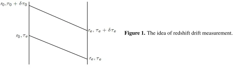
Redshift drift measurement [27] is to collect data from two light cones separated by 10-20 years to look for a change in redshift of a source as a function of time.
Figure 1.The idea of redshift drift measurement.
There is a relation between the times of emission of light by the sourcete andte+ Δte and the times of their observation attoandto+ Δtowhich in VSL theory generalizes into [28]
to
te
c(t)dt a(t) =
to+Δto
te+Δte
c(t)dt
a(t) , (25)
and for smallΔteandΔtotransforms into
c(te)Δte
a(te) =
c(t0)Δto
The definition of redshift in VSL theories remains the same as in standard Einstein relativity i.e. 1+z=a(t0)/a(te). Using (26) we have
Δz
Δt0 = Δz
Δt0
(z,n)=H0(1+z)−H(z)(1+z)n . (27)
In the limitn → 0 the formula (27) reduces to the one of the standard Friedmann universe [27]. Bearing in mind the definitions of dimensionless density parametersΩi, and assuming flat universe one has
H2(z)=H02Ωm0(1+z)3+ ΩΛ
(28)
and so (27) gives
Δz
Δt0 =H0
1+z− Ωm0(1+z)3+2n+ ΩΛ(1+z)2n
(29)
which can further be rewritten to define a new redshift function
˜
H(z)≡(1+z)nH(z)=H0
i=k
i=1
Ωwi(1+z)3(we f f+1) , (30)
wherewe f f = wi + 23n. The redshift drift can be measured by future telescopes such as E-ELT (European-Extremely Large Telescope), TMT (Thirty Meter Telescope), GMT (Giant Magellan Tele-scope) as well as gravitational wave detectors (DECIGO) DECi-Hertz Interferometer Gravitational Wave Observatory and BBO (Big Bang Observer).
0 1 2 3 4 5
40 30 20 10 0
z
10
10
z
15
year
CDM
n0.045
n0.045
n0.3 CDM
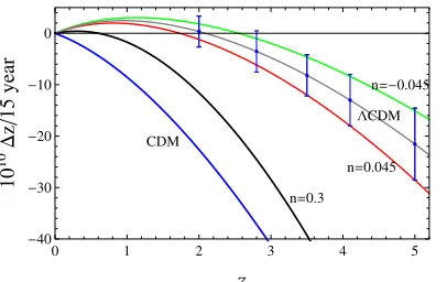
Figure 2.The redshift drift effect for 15 year period of observations for various values of the varying speed of light parameter n. The error bars are taken from [29] and presumably show that for|n| <0.045 one cannot distinguish between VSL models and
ΛCDM models.
This relation is presented in Fig. 2 from which one cas easily see that for small values of the parametern(small variation ofc) the dark energy can be mimicked while for large values ofnthere is a clear distinction between dark energy which can be detected.
4 Measuring
c
by future galaxy surveys
Speed of lightc appears in many observational quantities. Among them in the angular diameter distance [33]
DA=
DL (1+z)2 =
a0
1+z
t2
t1
c(t)dt
whereDLis the luminosity distance,a0present value of the scale factor (normalized toa0 =1 later),
and we have taken the spatial curvaturek =0 (otherwise there would be sin or sinh in front of the integral). Using the definition of redshift and the dimensionless parametersΩiwe have
DA = 1 1+z
z
0
c(z)dz
H(z) , (32)
where
H(z)= Ωr0(1+z)4+ Ωm0(1+z)3+ ΩΛ. (33)
4.1 Angular diameter distance maximum
Due to the expansion of the universe, there is a maximum of the distance at
DA(zm)=
c(zm)
H(zm), (34)
which can be obtained by simple differentiating (32) with respect toz:
∂DA
∂z =−
1 (1+z)2
z
0
c(z)dz H(z) +
1 1+z
c(z)
H(z) =0. (35)
In a flatk=0 cold dark matter (CDM) model, there is a maximum atzm=1.25 andDA≈1230 Mpc. For the standardΛCDM model of our interest the maximum is at 1.4<zm<1.8. The product ofDA andHgivesexactlythe speed of lightcat maximum (the curves intersect atzm):
DA(zm)H(zm)=c0 ≡299792.458 kms−1 (36)
if we believe it is constant (defined officially by Bureau International des Poids et Mesures (BIPM) [30] and a relative error is claimed to be 10−9[31]).
DA
c0
H
0.0 0.5 1.0 1.5 2.0 2.5 3.0
0 500 1000 1500 2000 2500 z DA H z L vs c0 ê H H z LH Mp c L zM
cHzML
0.0 0.5 1.0 1.5 2.0 2.5 3.0
0.0 0.5 1.0 1.5 z DA H z L H H z Lê c0
Figure 3.DAandH(z) crossing plots atzm.
Measuringzmis problematic if one uses DA only (this is because of a large plateau aroundzm which makes it difficult to avoid errors from small sample of data – besides, one has binned data, ob-servational errors, and intrinsic dispersion). However, one can appeal to an independent measurement ofc0/H(z) which is the radial (line-of-sight) mode of the baryon acoustic oscillations (BAO) surveys
for whichDA(z) is the tangential mode [32]. In other words, we have both tangential and horizontal modes as
yt=
DA
rs
, yr=
c Hrs
where
rs=
∞
zdec
ccs(z)dz
H(z) (38)
is the sound horizon size at decoupling andcs the speed of sound. The measurements of BAO are from BOSS DR11 CMASS [34]
DV
rs(zd) =13.85±0.17 at ¯z=0.57, (39)
where the volume-averaged distance is
DV =
⎡
⎢⎢⎢⎢⎣(1+z)2czD
2
A
H
⎤ ⎥⎥⎥⎥⎦13
, (40)
and from BOSS DR11 LOWZ [35]
DV =(1264±25)
rs(zd)
rs,f id(zd)
at ¯z=0.32. (41)
4.2 The method to measurec.
In Ref. [33] a new method to measurecbased on the relation (35) was proposed, and it is composed of the following steps:
1. Independently measuringDA(z) andH(z).
2. Calculatingzm.
3. Getting the productDA(zm)H(zm)=c(zm).
4. CalculatingΔc=c(zm)−c0, first assuming thatc(zm) may not be equal toc0.
5. Determining possible level of variability/constancy ofc.
For this sake the backgroundΛCDM model with an ansatz [36]
c(a)∝c0
1+ a
ac
n
(42)
is taken into account, whereacis the scale factor at the transition epoch from somec(a)c0(at early
times) toc(a)→c0(at late times to now). Three scenarios are considered [33]:
1) standard casec=c0;
2)ac=0.005,n=−0.01→Δc/c≈1% atz∝1.5;
3)ac=0.005,n=−0.001→Δc/c≈0.1% atz∝1.5. After using 103Euclid project [37] mock data simulations [38], one obtains the following results:
1)zm=1.592+−0.0390.043(fiducial model inputzm=1.596) andc/c0 =1±0.009;
2)zm=1.528+−0.0380.036(fiducialzm=1.532) andc(zm)/c0=1.00925±0.00831;
and
<c(zm)/c0−1σc(zm)/c0 >=1.00094
+0.00014
−0.00033, (43)
so thata possible detection by Euclid of1%variation at1σ-level in future will be possible. 3)zm=1.584+−0.0420.039(fiducialzm=1.589) andc(zm)/c0=1.00095±0.00852
and
<c(zm)/c0−1σc(zm)/c0 >=0.99243
+0.00016
−0.00013, (44)
4.3 Other surveys and perspectives
In fact, Euclid will have 1/10 of the error bars of the current missions like WiggleZ Dark Energy Survey (e.g. [39]). Other missions which will be competitive to Euclid and useful for our task will be: Dark Energy Spectroscopic Instrument (DESI) [40]; Square Kilometer Array (SKA) [41]; Wide-Field Infrared Survey Telescope (WFIRST) [42] (especially having largest sensitivity at potentialzmregion i.e. 1.5<z<1.6).
5 Conclusions
Varying speed of lightc(and related to them varying fine structure constantα) theories which attract more interest among physicists have both advantages as well as problems. The advantages of them is that they solve the flatness, horizon problems, and in some special cases, the singularity problem. However, their violation of Lorentz invariance leads to a choice of a preferred frame and a drop of standard variational principle. On the other hand,α-varying theories have better formulation and due to the definition ofα, they can be related to varying-ctheories.
In this paper we have proposed some new tests to check variability ofcin future telescope/space missions. The first was the redshift drift test which gives clear prediction for redshift drift effect which can potentially be measured by future telescopes like E-ELT, TMT, GMT, DECIGO/BBO. The second was to use baryon acoustic oscillations test and the Hubble function test to independently measure the radialDA and tangential modec/Hof the volume distance DV at the angular diameter distance maximumzm.
Putting this last method in simple terms we have considered a “cosmic” measurement of the speed of lightcwithDAgiving the dimension of length playing the role of a “cosmic ruler” and 1/H giving the dimension of time playing the role of a “cosmic clock”/”chronometer” i.e.
c= DA
1
H
. (45)
We have checked that 1% variability ofccan be tested at 1σlevel by Euclid mission. It is likely that such variability will also be possible to test by SKA and WFIRST.
Acknowledgements
The research of V.S., M.P.D., and A.B. was supported by the Polish National Science Center Grant DEC-2012/06/A/ST2/00395.
References
[1] P.A.M. Dirac, Nature139, 323 (1937); Proc. Roy. Soc. A165, 189 (1938). [2] C.H. Brans, R.H. Dicke, Phys. Rev.124, 925 (1961).
[3] J. Polchinski,String Theory(Cambridge University Press, Cambridge, 1998). [4] A. Einstein, Jahrbuch für Radioaktivität und Elektronik4, 411 (1907). [5] R.H. Dicke, Rev. Mod. Phys.29, 363 (1957).
[6] J.-P. Petit, Mod. Phys. Lett. A3, 1527 (1988). [7] J. Moffat, Int. J. Mod. Phys. D2, 351 (1993).
[8] A. Albrecht, J. Magueijo, Phys. Rev. D59, 043516 (1999). [9] J.K. Webb et al. Phys. Rev. Lett.87, 091301 (2001).
[11] J.D. Barrow, D. Kimberly, J. Magueijo, Class. Quantum Grav.21, 4289 (2004). [12] M.P. Da¸browski, K. Marosek, Journ. Cosmol. Astrop. Phys.02, 012 (2013).
[13] T. Cailleteau, J. Mielczarek, A. Burrau, and J. Grain, Class. Quantum Grav.29, 095010 (2012). [14] M.P. Da¸browski, K. Marosek, A. Balcerzak, Mem. Soc. Astron. Ital.85, 44-49 (2014).
[15] S. Nojiri, S.D. Odintsov and S. Tsujikawa, Phys. Rev. D71,063004 (2005). [16] M.P. Da¸browski, T. Denkiewicz, AIP Conference Proceedings1241, 561 (2010).
[17] M.P. Da¸browski, Mathematical Structures of the Universe, M. Eckstein, M. Heller, S.J. Szybka (eds.), (Copernicus Center Press, Kraków), 99 (2014).
[18] J.W. Moffat, arXiv: 1501.01872.
[19] J.K. Webb et al., Phys. Rev. Lett.107, 191101 (2011).
[20] P. Molaro, D. Reimers, I. I. Agafonova, S. A. Levshakov, Eur. Phys. JST163, 173 (2008). [21] H. Chand, R. Srianad, P. Petitjean, B. Aracil, R. Quast and D. Reimers, Astron. Astroph.451,
45 (2006).
[22] I. I. Agafonova, P. Molaro and S. A. Levshakov, Astron. Astroph.529, A28(2011). [23] P. Molaro et al., Astron. Astroph.555, A68 (2013).
[24] T. Rosenband et al., Science319, 1808 (2008).
[25] T. Denkiewicz, M.P. Da¸browski, C.J.A.P. Martins, P. Vielzeuf - Phys. Rev. D89, 083514 (2014). [26] M.P. Da¸browski, T. Denkiewicz, C.J.A.P. Martins, P. Vielzeuf - Phys. Rev. D89, 123512 (2014). [27] A. Sandage, Astrophys. J.136, 319 (1962); A. Loeb, Astrophys. J.499, L11 (1998).
[28] A. Balcerzak, M.P. Da¸browski, PLB728, 15 (2014). [29] C. Quercellini et al., Phys. Rep.521, 95 (2012). [30] www.bipm.org
[31] K.M. Evenson, Phys. Rev. Lett.29, 1346 (1972).
[32] S. Nesseris, L. Perivolaropoulos, Phys.Rev. D73, 103511 (2006).
[33] V. Salzano, M.P. Da¸browski, R. Lazkoz, Phys. Rev. Lett.114, 101304 (2015). [34] L. Samushia et al., Mon. Not. R. Astron. Soc.439, 3504 (2014).
[35] R. Tojeiro et al., arXiv: 1401.1768.
[36] J. Magueijo, Rep. Prog. Phys.66, 2025 (2003). [37] L. Laureijs et al. 0912.0914 (Euclid Collaboration).
[38] A. Font-Ribeira et al., Journ. Cosmol. Astropart. Phys.05, 023 (2014). [39] B.D. Sherwin, arXiv: 1207.4543.
[40] M. Levi et al., Astroph. Journ.803, 21 (2015). [41] Ph. Bull et al., 1405.1452)
![Table 1. The set of singularities for Friedmann geometry [15–17]](https://thumb-us.123doks.com/thumbv2/123dok_us/8154437.1360074/3.482.48.432.116.256/table-set-singularities-friedmann-geometry.webp)