Energy Optimization in Sensor Networks

(1)

CHIANG, MU-HUAN. Energy Optimization in Sensor Networks. (Under the direction of Gregory T. Byrd).

Recent advances in wireless communications and computing technology are enabling the emergence of low-cost devices that incorporate sensing, processing, and communication functionalities. A large number of these devices are deployed to create a sensor network for both monitoring and control purposes. Sensor networks are currently an active research area mainly due to the potential of their applications. However, the operation of large scale sensor networks still requires solutions to numerous technical challenges that stem primarily from the constraints imposed by simple sensor devices. Among these challenges, the power constraint is the most critical one, since it involves not only reducing the energy consumption of a single sensor but also maximizing the lifetime of an entire network. The network lifetime can be maximized only by incorporating energy awareness into every stage of sensor network design and operation, thus empowering the system with the ability to make dynamic tradeoffs among energy consumption, system performance, and operational fidelity.

Optimizing the energy usage is a critical challenge for wireless sensor networks (WSNs). The requirements of energy optimization schemes are as follows. (1) Low individual energy consumption: Sensor nodes can use up their limited energy supply, carrying out computations and transmission. In typical WSNs, nodes play a dual role as both data sender and data router. Malfunctioning of some sensor nodes due to power failure can cause significant topological changes and may require rerouting of packets and network reorganization. Therefore, reducing the energy consumption of each sensor node is critical for WSNs. (2) Balanced energy usage: While minimizing the energy consumption of individual sensor nodes is important, the energy status of the entire network should also be of the same order. If certain nodes have much higher workload than others, these nodes will drain off their energy rapidly and adversely impact the overall system lifetime. The workload of sensors should be balanced in order to achieve longer system lifetime. (3) Low computation and communication overhead: The resource limitations imposed by sensor hardware call for simple protocols that require minimal processing and a small memory footprint. The extra computation and communication introduced by the energy optimization schemes must also be kept low. Otherwise, energy required to perform the optimization schemes may outweigh the benefits.

This thesis concentrates on the energy optimization issues in wireless sensor networks. We study the power consumption characteristics of typical sensor platforms, and propose energy optimization schemes in network and application level. We design distributed algorithms that reduce the amount of data traffic and unnecessary overhear-ing waste in WSNs, and further propose load balancoverhear-ing mechanisms that alleviate the unbalanced energy usage and prolong the effective system lifetime.

(2)

(3)

by

Mu-Huan Chiang

A dissertation submitted to the Graduate Faculty of

North Carolina State University

in partial fulfillment of the

requirements for the Degree of

Doctor of Philosophy

Computer Engineering

Raleigh, North Carolina

2007

Approved By:

Dr. Peng Ning Dr. Mihail Sichitiu

Dr. Gregory T. Byrd Dr. Alexander G. Dean

(4)

Biography

Mu-Huan Chiang was born and raised in Taipei, Taiwan. After receiving his Master degree in Electrical Engineering from National Cheng Kung University in 2001, he served in the military as an Information Security Officer in National Security Bureau, Taiwan from 2001 through 2003.

(5)

Acknowledgements

First and foremost, I would like to thank my advisor, Dr. Gregory T. Byrd, for his encouragement, guidance, and support for the years I spent in NC State. I am grateful to Dr. Sichitiu, Dr. Dean, Dr. Ning, and Dr. Reeves for their valuable advice and constructive criticism which helped me through my research.

(6)

List of Figures

1.1 Conceptual diagram of a wireless sensor network. . . 2 1.2 Tmote Sky: (top) front side, (bottom) back side of the node [48]. . . 3

2.1 Components of energy consumption in radio communication [25] . . . 10 2.2 Radio energy per bit as a function of packet size and modulation level, using typical radio parameters

for sensor networks [63]. . . 11

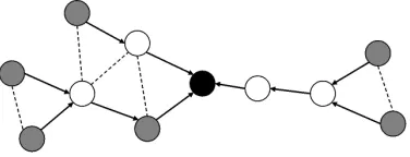
3.1 A simple routing tree, from source nodes (grey) to sink (black). Messages are received and retrans-mitted by forwarding nodes (white). Dotted lines are links that are available, but are not in the routing tree. Aggregation reduces message count from 15 to 10. . . 19 3.2 A minimal Steiner tree can use non-terminal (white) nodes to connect all terminal (black) nodes using

the minimal number of edges. The minimal Steiner tree is indicated by heavy line segments. . . 21 3.3 Snooping on neighborhood traffic. Node A overhears the message from X to Y, and can change its

parent from B to Y, to improve aggregation. . . 23 3.4 An example SPT and its corresponding AAT. Source nodes are represented by red circles. In AAT,

nodes can only select parents in the same level or one level up, which is loop-free if there are no loops in each level. The level in AAT is actually the level in SPT, which is not changed during the AAT parent switching process. . . 24 3.5 Three different aggregation trees for a sensor network. The network includes 1024 nodes with random

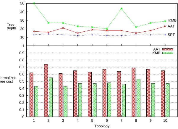
displacement from a320_×320grid. The green dotted lines represent the possible communication links. The dark lines represent paths used in the aggregation tree. The sink node is in the middle of the network, and 100 randomly-selected source nodes are shown as circles. . . 25 3.6 The tree depth of ten random networks, and the corresponding tree cost (normalized to the cost of SPT). 26 3.7 The average tree cost and depth with different number source nodes (10 simulation runs each). The

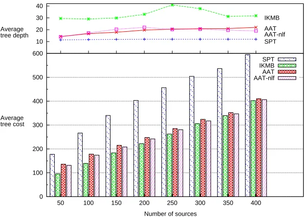
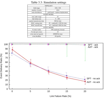
difference between AAT and AAT-nlf is not obvious, in terms of both cost and depth. When the number of sources increases, the cost of AAT becomes very close to IKMB. The tree cost reduction of AAT against SPT is around 34%, independent of the number of source nodes. The depth increase of AAT over SPT increases gradually with the number of sources, from 25% to 83%. . . 27 3.8 The packet sending/receiving process of AAT. The dark area shows the additional computation overhead. 32 3.9 Event delivery ratio versus link failure rate for AAT and SPT, with and without implicit

acknowledge-ments. . . 33 3.10 The timing of event delivery for AAT and SPT, with and without acknowledgements. . . 34 3.11 The components of energy consumption for communication for different link failure rates. The error

bar represents the variance on the total energy consumption for the 10 simulated networks. . . 35 3.12 The total communication energy consumption with different number of source nodes. The link failure

rate is 5%. The error bar represents the variance among the 10 simulated networks. The energy saving of AAT is around 23%, independent of the number of source nodes. . . 36 3.13 The comparison of the original GPSR and GPSR with AAT. The result is the average of 10 random

(10)

3.14 The energy consumption of GPSR and GPSR with AAT in networks with 5% link failure rate. The energy consumption for beacon packets are not included. The error bar represents the variance among the 10 simulated networks. The energy saving is around 31%, independent of the number of source

nodes. . . 38

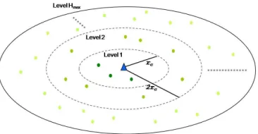
4.1 The network model for analysis. Hmaxis the maximum number of hops required to forward packets from the outermost nodes to the base station. . . 40

4.2 The average number of messages sent, received, and overheard by nodes in different levels, with and without aggregation, with fixedBt= 8andPS(k) = 0.01. . . 41

4.3 The average number of messages sent, received, and overheard by nodes in different levels, with and without aggregation, with fixedHmax= 15andPS(k) = 0.01. . . 42

4.4 State transitioning diagram of uniform density control. NB represents the number of neighbors, and Th represents the threshold value. . . . 46

4.5 Different neighborhood types in event-based sensor networks. The outermost rectangular area repre-sents the whole sensor field. . . 47

4.6 Percentage of dead nodes in areas in different levels of the network. The parenthesized number repre-sents the total number of sensor nodes in each area. . . 51

4.7 Four different lifetime indications of the simulation. . . 52

4.8 Distribution of sensor nodes with different energy consumption. . . 53

4.9 The timing of event delivery from 20 randomly chosen source nodes in the network. Each source sends one event at time 0. . . 53

4.10 The difference in the timing of event delivery from source nodes in different hops away from the base station. . . 54

4.11 Four lifetime indications of sensor networks with Adaptive Aggregation Tree accommodated. . . 55

4.12 The comparison of NADC and NADC with AAT. . . 55

4.13 Comparison of delivery delay from source nodes in different hops away from the base station. . . 55

5.1 Structured Replication . . . 60

5.2 Split-merge process . . . 62

5.3 Energy consumption of each sensor node in GHT-4, GHT-16, and Z-R . . . 66

5.4 Total energy consumption with varyingfHandQ(fL=₂₀₀₀1 ) . . . 68

5.5 Total energy consumption in 10-minute simulations . . . 69

(11)

List of Tables

1.1 Current consumption of Tmote Sky when active [48] . . . 5

3.1 Mica2 current consumption model . . . 32

3.2 Energy consumption estimation for Fig. 3.8 . . . 32

3.3 Simulation settings . . . 33

4.1 Power consumption (in mW) of Medusa II and Rockwell’s Wins nodes (with processor and sensor in active mode) [63] . . . 43

4.2 NADC states . . . 48

4.3 Network setting . . . 50

4.4 Statistics of the nodes’ energy usage in Fig. 4.8 . . . 52

5.1 Communication cost of External Storage (ES), Local Storage (LS), and Data-Centric Storage (DCS) . 59 5.2 Estimated total energy consumed by GHT and Z-R . . . 63

5.3 Simulation settings . . . 66

5.4 Hot-spot and total energy consumption . . . 67

(12)

Chapter 1

Introduction

Wireless sensor networks (WSN) [2] have emerged as a promising solution for various applications, in fields as diverse as climate monitoring, tactical surveillance, vehicle tracking, and earthquake detection. With improvements in sensor technology, it has become possible to build small sensor devices with a relatively high computational power at a low cost. Yet, the sensor devices’ untethered nature also poses interesting design challenges.

Energy consumption is the most important factor to determine the life of a sensor network, because usually sensor nodes are driven by batteries and have very low energy sources. This makes energy optimization more com-plicated in sensor networks; it involves not only reduction of energy consumption but also prolonging the life of the network as much as possible. This must be done by having energy awareness in every aspect of design and operation [34]. A single configuration may not fulfill the requirements to work energy-efficiently in different environments. Thus, mechanisms that can change adaptively in response to various situations are critical for energy efficiency in such systems.

This thesis concentrates on the energy optimization issues in wireless sensor networks. We study the power consumption characteristics of typical sensor platforms, and propose energy optimization schemes in network and application level. We design distributed algorithms that reduces the amount of data traffic and unnecessary overhearing waste in sensor networks, and further propose load balancing mechanisms that alleviate the unbalanced energy usage and prolong the effective system lifetime.

1.1 Wireless Sensor Networks

(13)

net-Figure 1.1: Conceptual diagram of a wireless sensor network.

works include environmental monitoring, natural disaster prediction, homeland security, health care, manufacturing, transportation, and home appliances and entertainment.

Conceptually, a wireless sensor network consists of a dense network of nodes as shown in Fig. 1.1. In typical deployment scenarios, a few neighboring nodes lie within the communication radius of each node. Each sensor node performs several functions such as (1) sensing the physical parameters of its environment, (2) processing the raw data locally to extract the feature of interest and (3) transmitting the information to its neighbors through a wireless link. Unlike cellular networks or wireless LAN, there are no distributed base stations or access points in wireless sensor networks. Hence, each node operates as a relay point to implement a multihop communication link by receiving data from one of its neighbor, and then processing it before routing it to the next neighbor towards the destination. In some cases, more functions such as data compression and encryption are also incorporated.

A common characteristic of many WSN application scenarios is that sensor nodes are deployed and tasked to monitor the environment. In particular, when sensor nodes detect a significant event, they are not expected to respond themselves. The prime reason is that some physical action is often required like sounding an alarm, adjusting some valves, or stopping an intruder, which would drain the batteries and increase the form factor significantly. A single sink can only serve a limited number of sensor nodes, so large deployments may include multiple sinks, each serving a patch of the nodes.

1.2 Challenges

The advances in wireless sensor networks, while promising, also have challenges, such as resource limita-tions, dynamic environment, and various application needs. These challenges and tradeoffs are discussed as follows.

1.2.1 Sensor Platform

(14)

Figure 1.2: Tmote Sky: (top) front side, (bottom) back side of the node [48].

figure shows, the main components of a typical sensor node include an antenna and a radio frequency (RF) transceiver to allow communication with other nodes, a memory unit, a CPU, the sensor unit, and the power source which is usually provided by batteries. Although their limited size makes them attractive for use in a number of situations, the small size limits battery capacity requiring every operation to be done efficiently. It also limits the radio transmission range and suggests a small multihop transmission structure.

The power restrictions of sensor nodes are raised due to their small physical size and lack of wires. Since the absence of wires results in lack of a constant power supply, not many power options exist. Sensor nodes are typically battery-driven. The power is used for various operations in each node, such as running the sensors, processing the information gathered and data communication. An alternative power source of sensor nodes is energy scavenging from ambient sources [56]. Although many different techniques are available to harvest energy from various environments to power electronics, the amount of available raw energy (for example, sunlight, vibration, heat) and the surface area or net mass that the sensor permits limit the power yield. Therefore, the derived energy from scavenging is still limited.

In the case of computational power, computations are linked with the available amount of power. Since there is a limited amount of power, computations are constrained. The storage size is also limited due to the power and physical size of sensor nodes.

1.2.2 Network Construction and Maintenance

(15)

deployed systems must be designed to operate under environmental dynamics while preserving the sensing coverage and network connectivity.

In some WSN applications, the large number of elements in the network and the harsh environment make the maintenance operations (e.g., recharge depleted batteries, replace failed nodes) prohibitively expensive. In such contexts some mechanisms are required to maintain the system performance and operational fidelity when sensor nodes fail or deplete their limited energy.

1.2.3 Data Dissemination and Collection

Basic capabilities in WSN involve mechanisms of disseminating information over many nodes and collecting data to a sink node. Due to the power restrictions and environmental dynamics of WSN, these mechanisms have to be low power, scalable with the number of nodes, and fault tolerant to nodes that go up or down, or move in and out of range. Moreover, some sensor nodes may fail or be blocked due to lack of power, physical damage, or environmental interference. If many nodes fail, some mechanisms must accommodate formation of new links and routes to the data collection sinks. This may require actively adjusting transmit power to change the existing topology, or rerouting packets through regions of the network where more energy is available.

1.3 The Need for Energy Optimization in WSN

One of the most important limitations of sensor networks is energy conservation. Wireless sensors operate on limited power sources, therefore, their main focus is on power conservation through appropriate optimization of communication and operation management. Energy awareness must be incorporated into groups of communicating sensor nodes of the entire network as well as into the individual nodes. Especially for systems such as intrusion detection and target tracking, where long periods of minimal sensing activity are intermixed with short periods of intense sensor processing, workloads are highly irregular both spatially and temporally.

The energy consumption in WSN involves three main components: Sensing Unit (Sensing transducer and A/D converter), Communication Unit (transmission and receiver radio), and Computing/Processing Unit. Between sensing, computational and communication, the power consumption needed for communication typically dominates a node’s power budget. Table 1.1 shows a breakdown of the current consumption of a state-of-the-art sensor node when active. The corresponding power consumption can be derived by multiplying the current consumption with the voltage supply (about 3V). The results indicate that the power consumption of transmitter and receiver is much higher than the other components. To overcome this bottleneck, it is critical to reduce the power consumption for communication, and the research in this thesis focuses on the optimization of energy usage for communication.

1.3.1 Requirements

(16)

Table 1.1: Current consumption of Tmote Sky when active [48] Components Active current consumption (mA) Condition

Transmitter 17.4 0 dBm output power

Receiver 19.7 -94 dBm Rx sensitivity

Microprocessor 0.5 3V supply, 1MHz clock

Sensors <0.03

-Voltage regulator 0.02

-• Low individual energy consumption — Sensor nodes can use up their limited energy supply, carrying out

computations and transmission. In a multihop WSN, nodes play a dual role as data sender and data router. Malfunctioning of some sensor nodes due to power failure can cause significant topological changes and might require rerouting of packets and reorganization of the network. Therefore, reducing the energy consumption of each sensor node is critical for WSNs.

• Balanced energy usage — While minimizing the energy consumption of individual sensor nodes is important,

the energy status of the entire network should also be of the same order. If certain nodes have much higher workload than others, these nodes will drain off their limited energy rapidly and adversely impact the lifetime of the overall system. The workload of sensors should be balanced in order to achieve longer system lifetime.

• Low computation and communication overhead — The resource limitations imposed by typical node

hard-ware call for simple protocols that require minimal processing and have a small memory footprint. The extra computation and communication introduced by the energy optimization schemes must also be kept low. Other-wise, energy required to perform the optimization schemes may outweigh the benefits.

1.3.2 State of the Research

There already exist some efforts to overcome the challenges in reducing energy consumption and extending system lifetime in wireless sensor networks. The proposed optimization approaches can be divided into three different categories:

1. Low power sensor architecture [47, 51, 62]: As a first step towards incorporating energy awareness into the network, it is necessary to develop hardware/software design methodologies and system architectures that enable energy-aware design and operation of individual sensor nodes in the network.

2. Energy-efficient communication [59, 94, 49, 86]: While the optimization of individual sensor nodes reduces en-ergy consumption, it is important for the communication between nodes to be conducted in an enen-ergy-efficient manner as well. Since the wireless transmission of data accounts for a major portion of the total energy con-sumption, optimization schemes that take into account the effect of inter-node communication yield significantly higher energy savings. Furthermore, incorporating energy optimization into the communication process enables the diffusion of energy awareness from an individual sensor node to a group of communicating nodes, thereby enhancing the lifetime of entire regions of the network.

(17)

groups of communicating nodes alone does not solve the energy problem in sensor networks. The network as a whole should be energy aware, for which the network-level global decisions should be energy aware.

Some state-of-the-art optimization schemes will be presented in Chapter 2.

1.4 Contributions and Scope of this Thesis

The previous sections have discussed the main challenges in wireless sensor networks and the need for energy optimization schemes. The requirements of energy optimization schemes are (1) node’s individual energy consumption has to be low to adapt to the limited energy source, (2) the workload of nodes should be kept of the same order for balanced energy usage, and (3) the computation and communication overhead must be low to meet the nodes’ resource limitations. Existing strategies are usually tightly coupled with network protocols and other system functionality, and only provide point solutions which are insufficient for these highly energy-constrained systems. Energy optimization, in the case of sensor networks, is much more complex, since it involves not only reducing the energy consumption of a single sensor node but also maximizing the lifetime of an entire network. The network lifetime can be maximized only by incorporating energy awareness into every stage of wireless sensor network design and operation, thus empowering the system with the ability to make dynamic tradeoffs between energy consumption, system performance, and operational fidelity.

The thesis focuses on energy optimization for wireless sensor networks from various perspectives. It con-tributes to the advancement of energy optimization in the following two major thrusts:

1. Exploit overhearing effect to improve aggregation efficiency and network energy management Owing to the broadcast nature of the wireless channel, many nodes in the vicinity of a sender node may overhear its packet transmissions even if they are not the intended recipients of these transmissions. This redundant reception results in unnecessary expenditure of battery energy of the recipients. Especially in dense sensor networks, overhearing costs can constitute a significant fraction of the total energy consumption.

Overhearing problem is common in wireless sensor networks. Although several WSN MAC protocols have been proposed using short control packets to avoid overhearing long data packets, overhearing the control packets still consumes considerable overhead energy. Since overhearing is difficult to avoid and sometimes necessary, we propose distributed energy optimization schemes which exploit the overhearing effect as an approach to gather the required information.

Adaptive Aggregation Tree (AAT) is proposed to dynamically transform the routing tree, using

easily-obtained overheard information, to improve the efficiency of data aggregation. Based on the simple shortest-path tree, AAT allows each node to adaptively choose a new parent if it appears to provide better opportunities for aggre-gation. The local adaptivity of AAT successfully reduces the number of message transmissions and achieves a 20% energy reduction, compared to the shortest-path tree where aggregation occurs opportunistically.

Neighborhood-Aware Density Control (NADC) exploits the overheard information to reduce the unnecessary

(18)

keeping the nodes involved in packet generation or forwarding in the active state, the overhearing waste can be reduced without dramatically increasing the delay of event delivery.

2. Extend system lifetime through load balancing Due to the multihop routing nature of sensor networks, the nodes along the routing paths tend to have heavier workload and deplete their energy sources faster than other nodes. Especially in densely deployed sensor networks, the overhearing cost may aggravate the unbalanced energy usage among sensor nodes. Such unbalanced energy usage leads to a premature loss of connectivity in the network and negatively impacts the system lifetime.

In this thesis, the unbalanced energy usage problem is attacked from two perspectives. In the network level, NADC reduces the unnecessary overhearing along routing paths and alleviates the unbalanced energy usage among sensor nodes. In the application level, we propose Zone-Repartitioning (Z-R) for load balancing in data-centric storage systems. Z-R reduces the energy consumption of certain hot-spots by distributing their communication load to other nodes when the event frequency of certain areas is much higher than the others.

(19)

Chapter 2

Energy Optimization Schemes in WSN

2.1 Low Power Sensor Architecture

Energy consumption in an arbitrary sensor node has in general the following components depending on the operations performed within the node:

1. Sensing energy: Sensing energy must be dissipated in order to activate sensing circuitry and gather data from the environment. The magnitude of this energy depends on the task that is assigned to the sensor. Different sensors require different levels of energy during operation.

2. Communication energy: A node consumes communication energy while sending or forwarding data packets to the base station. The communication energy includes transmission energy and receiving energy.

3. Computation energy: To operate the sensor node, the sensor’s processor/microcontroller must be activated. Moreover, whenever data aggregation is performed, additional computations must be realized. Compared to the previous items, computation energy is usually relatively low.

The low power design of sensor nodes is one of the most crucial aspects of sensor network energy optimization. Ultimately, it is the sensor node hardware that consumes the energy, so if the node itself is not energy-efficient, no amount of higher layer optimization will yield desired results. While the sensing energy is dependent on the sensing requirements in different applications, various approaches have been proposed to reduce the computation and communication energy consumption.

2.1.1 Power-Aware Computing

Dynamic Power Management Dynamic power management (DPM) [8] is an effective tool in reducing system

(20)

needed and wake them up when necessary. DPM, in general, is not a trivial problem. If the energy and performance overheads in sleep state transition were negligible, then a simple greedy algorithm that makes the system enter the deepest sleep state when idling would be perfect. However, in reality, sleep-state transitioning has the overhead of storing processor state and turning off power. Waking up also takes a finite amount of time. Therefore, implementing the correct policy for sleep-state transitioning is critical for DPM success.

Dynamic Voltage Scaling While shutdown techniques can yield substantial energy savings in idle system states,

additional energy savings are possible by optimizing the sensor node performance in the active state. Dynamic voltage scaling (DVS) [96] is a popular approach to power and energy reduction in microprocessors. Many modern processors are designed to operate at different voltage and frequency settings as an effective way to mange power usage. As the processor frequency is reduced, the supply voltage can also be reduced. As shown by the equations below, the reduction in frequency combined with a quadratic reduction from the supply voltage results in an approximately cubic reduction of power consumption. However, with educed frequency, the time to complete the task increases, leading to an overall quadratic reduction in the energy required to complete a task. DVS is therefore an effective method to reduce the energy consumption of a processor.

Delay= 1

f = CsVdd

Idsat ∝

Vdd (Vdd−Vth)1.3

P ower_∝f Vdd2

Energy_∝Vdd2

In most current processor designs, the voltage range is limited from fullVddto approximately halfVddat

most. Research has indicated that extending the operating voltage range, even to subthreshold voltages, may improve the energy efficiency for many processor designs. However, significant design effort is required to accommodate operation over a wide range of voltage levels. Furthermore, the landscape for microarchitectural energy optimization dramatically changes in the subthreshold domain, which limits the possible maximum savings DVS can approach [85].

Subthreshold-Voltage Circuits Many sensor network applications have low performance requirements and the

pro-cessors only execute low-performance tasks intermittently. Superthreshold (Vdd> Vth) circuit implementations are

sometimes too fast and energy-hungry for these applications [51]. Since optimal supply voltage to minimize energy typically occurs in the subthreshold (Vdd< Vth) region with reduced performance, several subthreshold

micropro-cessors have been proposed trying to operate from energy scavenged from the ambient environment.

(21)

2.1.2 Energy-Aware Software

The OS is ideally poised to implement shutdown-based and DVS-based power management policies, since it has global knowledge of the performance and fidelity requirements of all the applications and can directly control the underlying hardware resources, fine tuning the available performance-energy control knobs. At the core of the OS is a task scheduler, which is responsible for scheduling a given set of tasks to run on the system while ensuring that timing constraints are satisfied. System lifetime can be increased considerably by incorporating energy awareness into the task scheduling process.

TinyOS [28] is an operating system specifically designed to address the needs of wireless sensor networks. It is based on an event driven execution engine that simultaneously provides efficiency and fine-grained concurrency. TinyOS’s event based communication is encapsulated in a component model that allows state-machine based compo-nents to be efficiently composed together into application-specific configurations. The TinyOS communication system is based on the Active Messages communication paradigm taken from high-performance computing environments. When data is received from the network, message-specific handlers are automatically invoked.

2.1.3 Energy-Efficient Radio Transceiver

While power management of embedded processors has been studied extensively, incorporating power aware-ness into radio subsystems has remained relatively unexplored. Energy-efficient radio transceiver is extremely impor-tant since wireless communication is a major power consumer during system operation. As shown in Figure 2.1, the power consumed by radio has two main components[25]:

1. An RF component that depends on the transmission distance and modulation parameters.

2. An electronics component that accounts for the power consumed by the circuitry that performs frequency syn-thesis, filtering, up-converting, etc.

Figure 2.1: Components of energy consumption in radio communication [25]

(22)

Figure 2.2: Radio energy per bit as a function of packet size and modulation level, using typical radio parameters for sensor networks [63].

2.2 Energy-Efficient Communication

While power management of individual sensor nodes reduces energy consumption, it is important for the communication between nodes to be conducted in an energy efficient manner as well. Since the wireless communica-tion of data accounts for a major porcommunica-tion of the total energy consumpcommunica-tion, power management decisions that take into account the effect of inter-node communication yield significantly higher energy savings.

2.2.1 Modulation Schemes

Besides the hardware architecture itself, the specific radio technology used in the wireless link between sensor nodes plays an important role in energy consideration. The choice of modulation scheme greatly influences the overall energy versus fidelity and latency tradeoff that is inherent to a wireless communication link. Fig. 2.2 plots the communication per bit as a function of the packet size and the modulation level. The optimal modulation level for each packet size is relatively high, close to 16-QAM (4 bits per symbol) for the radio parameters used. Higher modulation levels might be unrealistic in resource constrained sensor nodes. In these scenarios, a practical guideline for saving energy is to transmit as fast as possible at the optimal setting, and shut off the transmitter during the idle period [86].

(23)

2.2.2 Energy-Efficient MAC Protocols

Medium-access control (MAC) protocols for wireless networks manage the usage of the radio interface to ensure efficient utilization of the shared bandwidth. MAC protocols designed for WSNs have an additional goal of managing radio activity to conserve energy. While traditional MAC protocols must balance throughput, delay, and fairness concerns, WSN MAC protocols place an emphasis on energy efficiency as well. There are several aspects of a traditional MAC protocol that have a negative impact on wireless sensor networks, including:

• Collisions — When a transmitted packet is corrupted due to a collision, it has to be discarded. The follow-on

retransmission increases the energy consumption.

• Overhearing — Nodes receive packets that are destined to other nodes.

• Control packets overhead — Sending and receiving control packets consumes extra energy. Moreover, as more

nodes fail in the network, more control messages are required to reconfigure the system, resulting in more energy consumption.

• Idle listening — Waiting to receive anticipated traffic that is never sent.

WSN MAC protocols generally reduce energy consumption by putting radios to a low-power sleep mode, either periodically or whenever possible when a node is neither receiving nor transmitting. An important consequence is that a node needs to be aware of its neighbors’ sleep/active schedules, since sending a message is only effective when the destination node is awake. An obvious solution is to have all nodes synchronize on one global schedule, so no separate neighbor state is required, which maps well onto the resource limitations of typical sensor nodes. However, grouping communication into small (active) periods requires precise time synchronization and may increase the chance of collisions, so other forms of organization have been proposed.

The MAC protocols for sensor networks can generally be divided into two categories: schedule-based and

contention-based. In schedule-based protocols, energy waste due to overhearing, collision, idle listening, and

transi-tions between different states can be minimized. In addition, schedule-based medium arbitration can enhance delay predictability and limit packet drops due to interference and buffer overflow. However, the problem of scheduling access to the medium is NP-hard [75, 65], making the scalability of schedule-based MAC schemes a major concern. Distributed schedule-based medium arbitration typically introduces excessive overhead, and maintaining clock syn-chronization among nodes is essential to enforce the schedule – this is a non-trivial problem for resource-constrained sensor nodes.

Contention-based protocols do not divide and pre-allocate the channel into sub-channels for each node to use. Instead, a common channel is shared by all nodes, and it is allocated on-demand. A contention mechanism is employed to decide which node has the right to access the channel. These protocols are not as energy-efficient as schedule-based protocols, but they have several advantages. First, they scale more easily across changes in node density or traffic load. Second, they are more flexible as topologies change. Finally, they do not require fine-grained time synchronization. Due to the highly dynamic and untethered nature of sensor networks, these advantages make contention-based protocols the preferred choice, and they have been widely adopted.

(24)

Asynchronous Sleep Techniques In these techniques nodes normally keep their radios in sleep mode as a default, waking up briefly only to check for traffic or to send/receive messages. Nodes need to be able to sleep to save energy when they do not have any communication activity and be awake to participate in any necessary communications.

A hardware solution is to equip each sensor node with two radios [79, 73]. The primary radio is the main data radio, which remains asleep by default. The secondary radio is a low-power wake-up radio used for signalling. If the wake-up radio of a node receives a wake-up signal from another node, it responds by waking up the primary radio to begin receiving. This ensures that the primary radio is active only when the node has data to send or receive. Since the wake-up radio need not do much sophisticated signal processing, it can be designed to be extremely low power. A tradeoff, however, is that all nodes in the broadcast range of the transmitting node may be woken up.

Another solution is to use preamble sampling or low-power listening, in which the receivers periodically wake-up to sense the channel. If no activity is found, they go back to sleep. If a node wishes to transmit, it sends a preamble signal prior to packet transmission. Upon detecting such a preamble, the receiving node will change to a receiving mode. An implementation of this class of protocols is B-MAC [59] protocol. It provides a limited set of core functionality and an interface that allows the core components to be tuned and configured depending on higher-layer needs. The core B-MAC consists of the following features:

• Low-power listening (LPL), which implements the preamble-based wake-up to permit nodes to have sleep as the default mode, helping to conserve energy. Different channel sampling durations and preamble durations can be selected by the higher layers.

• Clear channel assessment (CCA), which determines whether the channel is busy or not by examining multiple adjacent samples and using an appropriate outlier detection technique.

• Acknowledgements (ACK): If acknowledgements are enabled, a response is sent immediately after receiving any unicast packet.

A desirable feature of B-MAC is that it is designed in a modular fashion and provides core functionality that enables easy implementation of other more complex MAC protocols over B-MAC. For example, channel reservation signals for RTS/CTS (Request to Send / Clear to Send) can be implemented above B-MAC using its control interfaces, but are not part of the core B-MAC itself.

Low-power listening/preamble sampling has one potential shortcoming: the long preamble that the transmit-ter needs to send can cause throughput reduction and energy waste. The WiseMAC [22] protocol builds upon preamble sampling to correct this deficiency. Using additional contents of ACK packets, each node learns the periodic sampling times of its neighboring nodes, and use this information to send a shorter wake-up preamble at just the right time.

Sleep-Scheduled Techniques A typical protocol of this class of techniques is Sensor-MAC (S-MAC) [94]. Its basic

(25)

consumption. However, low-duty-cycle operation reduces energy consumption at the cost of increased latency, since a node can only start sending when the intended receiver is listening.

T-MAC [84] extends S-MAC by dynamically adjusting the duration between sleep intervals in which sensors are awake based on communication of nearby neighbors. In order to reduce number for switching, T-MAC introduced additional overhead control packets to prevent nodes from early sleep switching. D-MAC [42] addresses the latency overhead of S-MAC for the convergecast communication pattern, be staggering receive/send slots according to the level in the tree. It uses CSMA with ACKs to arbitrate between children, and schedules overflow slots whenever a message is received.

Z-MAC [68] is a hybrid scheme that starts off as CSMA but switches to TDMA when the load increases. Nodes run a distributed slot selection algorithm and the owner of a slot gets precedence by using as small random back-off value. Since all nodes must listen to all slots, Z-MAC builds on LPL for energy efficiency.

2.2.3 Energy-Reliability Tradeoff

Reliable delivery of data is a classical design goal for all network infrastructures. Guaranteed packet delivery is ensured by the careful selection of error free links, avoidance of overloaded nodes, and the detection and the recovery from packet drops. There is usually a tradeoff between the control traffic overhead and the level of reliability.

Implicit Acknowledgement Due to environmental interference and packet collisions, link failures and packet losses

are inevitable in sensor networks. Although sensor networks may indeed tolerate a certain amount of data loss without significantly affecting the aggregate, for the system to scale, the fraction of delivered packets should remain finite and representative of the original pool. That means a certain degree of reliability is needed, especially when hop count increases, because a single lost packet may result in loss of a large amount of aggregated data.

A simple solution to improve packet delivery is to use explicit acknowledgement packets or signals. If the sender does not receive an ack from the receiver within a timeout period, it assumes that either the data packet or the ack is lost, and sends the data packet again. This solution is intuitive, and has proved to be robust in practice. However, the extra energy required to send and receive the acks makes this scheme unattractive to sensor networks. Implicit

acknowledgement [9] reduces this extra energy consumption by embedding the acknowledgement into regular data

packets. When a node receives packets from its upstream nodes, instead of sending back explicit acknowledgement packets, the acks are piggybacked on the aggregated data packet destined to the next hop. Based on the broadcasting nature of wireless links, the upstream nodes can usually overhear this packet and get the acks.

Adaptive Error Correction Adaptive error correction schemes were proposed to reduce energy consumption while

(26)

2.3 Lifetime-Aware Energy Management

Incorporating energy awareness into individual nodes and pairs of communicating nodes alone does not solve the energy problem in sensor networks. There is significant research activity to minimize energy dissipation at the system level to lengthen battery lifetimes for WSN applications.

2.3.1 In-Network Processing

Many applications in WSNs require processing of the raw data collected by spatially distributed sensors. The tradeoffs between communication and computation energy have shown that in-network processing [44, 37] of the sensed data is more energy efficient than transferring the raw data to the powerful base station for processing. With in-network processing, data messages from neighboring nodes are combined into a single message on their way to the base station. Depending on the type of data being collected, the processing can be simple (e.g., send the maximum of all incoming data) or complex (e.g., compute a compressed or hashed version of incoming data). Even simply concatenating individual data messages into a single, larger message can result in energy savings, because the startup cost of a message transmission can be significant. The details of in-network processing and its related techniques will be discussed in Chapter 3.

2.3.2 Data-Centric Storage

Current industrial and scientific uses of wireless sensor networks can be classified broadly along two di-mensions: queries on live data and queries on historical data. In live data querying, sensor samples are useful within a small windows of time after they have been acquired. Querying historical data is required for applications that need to mine sensor logs to detect unusual patterns, analyze historical trends, and develop better models of particular events. While a large class of energy-efficient techniques have been proposed for querying live data, the management of historical sensor data also requires energy-efficient solutions.

There are two models for designing such historical data querying systems. The first model treats sensor data as a continuous stream that is aggregated within the network and then transmitted and archived outside the sensor network. Once the data is collected, they can be stored in a traditional database, and queried using standard techniques. While such a model is easy to deploy, these deployments can be short-lived when high data rate sensors (e.g., camera, acoustic, or vibration sensors) are used, since the data communication requirements overwhelm the available energy resources.

(27)

2.3.3 Traffic Distribution

Routing protocols for WSNs have been extensively studied in the last few years. Many routing, power management, and data dissemination protocols have been specifically designed for WSNs where energy awareness is an essential design issue. Routing protocols in WSNs might differ depending on the application and network architecture, and various energy optimization approaches have been proposed for these routing protocols.

Some of these approaches were proposed to select paths that minimizes the total energy consumption. How-ever, such a strategy does not always maximize the network lifetime. Consider a target-tracking application. While forwarding the gathered and processed data the base station, it is desirable to avoid routes through regions of the network that are running low on energy resources, thus preserving them for future, possibly critical detection and communication tasks. So it is in general undesirable to continuously forward traffic via the same path, even though it minimizes the energy, up to the point where the nodes on that path are depleted of energy, and the network connec-tivity is compromised. Therefore, some energy-aware routing protocols have been proposed to spread the load more uniformly over the network while trying to minimize the total energy consumption [74, 13].

The basic idea of energy-aware routing is that to increase of lifetime of networks, it may be necessary to use sub-optimal paths occasionally. This ensures that the optimal path does not get depleted and the network degrades gracefully as a whole rather than getting partitioned. To achieve this, multiple paths are found between source and destinations, and each path is assigned a probability of being chosen, depending on the energy metric. By employing this mechanism, the nodes in the primary path do not deplete their energy resources through continual use of the same route, hence prolonging their lifetime.

2.3.4 Topology Management

The core functionality of a wireless sensor network depends on having a network topology that satisfies two important objectives: coverage and connectivity. Coverage pertains to the application-specific quality of information obtained from the environment by the networked sensor nodes. Connectivity pertains to the network topology over which information routing can take place.

The problem of constructing an initial topology is the problem of node deployment. There are two major methodologies for deployment: (a) structured placement and (b) random scattering of nodes. Particularly for small-medium-scale deployments, where there are equipment cost constraints and a well-specified set of desired sensor locations, structured placements are desirable. In other applications involving large-scale deployments of thousands of inexpensive nodes, such as surveillance of remote environments, a random scattering of nodes may be the most flexible and convenient option. Nodes may be over deployed, with redundancy for reasons of robustness or ease of future maintenance [12].

Beyond initial deployment of sensor nodes, there are many scenarios in which topology control is desired. Topology control can be defined as the process of configuring or reconfiguring a network’s topology through tunable parameters after deployment. There are three major tunable parameters for topology control:

Node Mobility In WSNs consisting of mobile nodes, such as robotic sensor networks [7], both coverage and

(28)

Transmission Power Control If the deployment density is already sufficient to guarantee the required level of coverage, the connectivity properties of the network can be adjusted by tuning the transmission power of the constituent nodes. Power control is quite a complex and challenging cross-layer issue. Increasing radio transmission power has a number of interrelated consequences – some of these are positive, others negative:

• It can extend the communication range, increasing the number of communicating neighboring nodes and im-proving connectivity in the form of availability of end-to-end paths.

• For existing neighbors, it can improve link quality (in the absence of other interfering traffic).

• It can induce additional interference that reduces capacity and introduces congestion.

• It can cause an increase in the energy expended, due to the higher transmitting power and increased overhearing waste.

Many algorithms have been developed for variable power-based topology control [64, 55]. Power control techniques must provide connectivity, while taking into account diverse factors, including interference minimization and energy reduction.

Density Control Density control is an approach that controls the density of working sensors at a desirable level. It

(29)

Chapter 3

Reduction of Communication Energy

Consumption

In order to achieve reasonable lifetimes, sensor networks need to conserve energy, and an important com-ponent of energy usage in these systems is the wireless communication among sensor nodes [27]. Therefore, much research is focused on reducing the total number of messages in the network.

One particular approach is to use in-network data aggregation [44, 37], in which data messages from neigh-boring nodes are combined into a single message on their way to the data collection node. Depending on the type of data being collected, the aggregation can be simple (e.g., send the maximum of all incoming data) or complex (e.g., compute a compressed or hashed version of incoming data). Even simply concatenating individual data messages into a single, larger message can result in energy savings, because the startup cost of a message transmission can be significant.

A persistent sensor network query is initiated by a sink node, which then collects all of the data from other sensors. Sensor nodes that have data to report are called source nodes, and data messages are relayed to the sink using the network’s routing protocol. Nodes that transmit the data on behalf of source nodes, but which do not generate data themselves, are forwarding nodes. The “persistent” nature of the query means that source nodes are expected to periodically send event messages until the query expires or is cancelled.

Without aggregation, every source sends a data message to the sink, and forwarding nodes may relay mes-sages from several sources. If aggregation is allowed, a forwarding node may opportunistically notice that it is on the routing path between multiple source nodes and the sink. It can then start combining messages from those nodes. Fig. 3.1 shows a simple routing tree example.

(30)

they could choose a routing tree that maximizes aggregation and minimizes the total number of messages.

We discuss such trees in Section 3.1, but for now we will just say that selecting an optimal tree would be very expensive, since it requires the exchange of topology information among nodes. Furthermore, the number of source nodes and their locations are usually unpredictable and highly dynamic. The expense of re-calculating an optimal tree for each new set of source nodes would quickly swamp the benefit gained by more efficient aggregation.

The goal is to adaptively and dynamically transform a simple routing tree, using easily-obtained local infor-mation, to improve the efficiency of aggregation. The main idea is that a node can acquire neighborhood information by hearing beacon packets or overhearing messages transmitted in the same locality. By observing these messages, the node can determine whether it can change its route to increase shared links with other active paths. The details are described in Section 3.2, along with implementation issues in Section 3.3.

Our results in Section 4.4 show that this local adaptivity achieves significant energy reduction, compared to the opportunistic approach discussed above. This approach is especially beneficial to systems that monitor event-driven phenomena, such as traffic monitoring or wildlife tracking systems, where the source nodes change over time, favoring a simple adaptive scheme.

3.1 Background

3.1.1 Query Processing in Sensor Networks

In a sensor network, the sensors typically collect and transmit information periodically, and have to carefully manage limited power to ensure that essential information is collected and reported in a timely fashion. Several sensor query processing architectures, such as TinyDB [45] and Cougar [93], have been proposed to facilitate fast development of such data collection applications. In these architectures, users compose queries specifying the data they wish to collect and how they wish to combine, transform, and summarize it. In such queries, extracting all data over all time from all sensors will consume large amounts of energy as each individual sensor’s data is independently routed through the network. There are several approaches, such as packet merging, grouping, and data caching, to solve the problem [92], and data aggregation has been proposed as a particularly useful paradigm to reduce network traffic.

In a sensor query processing system, a communication architecture is required for query dissemination and result collection. A routing tree is a communication primitive rooted at either the base station or a storage point. The

(31)

root is the point from which the routing tree will be built, and upon which aggregated data will converge. The root first broadcasts a query message, asking sensors to organize into a routing tree; in that message it specifies its own ID and its level (distance from the root), which is zero. Any sensor that hears this message assigns its own level to be the level in the message plus one, if its current level is not already less than or equal to the level in the message. It also chooses the sender of the message as its parent, through which it will route messages to the root. These sensors then rebroadcast the routing message, inserting their own IDs and levels. The routing message floods the whole network in this fashion, until all nodes have been assigned a level and a parent. Nodes that hear multiple parents choose one arbitrarily or based on certain rules. When a sensor wishes to send a message to the root, it sends the message to its parent, which in turn forwards the message to its parent, and so on, eventually reaching the root.

A node can generally choose a parent from several possible candidate nodes; a simple approach is to choose the ancestor node at the lowest level or with the shortest delay. In practice, however, choosing a proper parent is quite important in terms of communication and data collection efficiency.

3.1.2 Data aggregation

Data aggregation is a way to combine data from different sources. The simplest data aggregation function is duplicate suppression - if multiple sources all send the same data and only one is required, these data items can be aggregated together. Other aggregation functions could be min, count, average, or even a user-defined function with multiple inputs, as long as the function is decomposable. A function is decomposable if it can be computed by another function as follows:

f(v1, v2, ..., vn) =g(f(v1, ..., vk), f(vk+1, ...vn))

Using decomposable functions, the value of the aggregate function can be computed for disjoint subsets, and these values can be used to compute the aggregate of the whole set, using the merging functiong. In this approach, after the queries are distributed across the network, aggregate results are sent back to the querier over a spanning tree, with each sensor combining its own data with results received from its children.

If there are no failures, this in-network aggregation technique is both effective and energy-efficient. How-ever, a high loss rate is inevitable on wireless links, and this effect accumulates quickly as the number of hops increases. For example, when loss rate is 5% per hop, the loss rate after 10 hops becomes 40%. The effect becomes more severe when aggregation is used because a single packet loss results in the loss of all aggregated data in that packet. Thus a reliable transmission scheme is critical for efficient data aggregation.

3.1.3 Aggregation Trees

In this section, we introduce several aggregation trees and their characteristics.

Shortest-Path Tree

(32)

nodes on the list with lower level can be the candidate nodes for parent selection. If delay is used as the criterion of parent selection (i.e. choose a candidate node which has the lowest level), the resulting tree will be a shortest-path tree. There is nearly no additional computation or communication required for the construction of SPT, and hence it is the easiest way to form an aggregation tree.

In this data aggregation scheme, each source node sends its information to the sink node along the shortest path. Where these paths overlap for different source nodes, they are combined to form the aggregation tree. Since the primary goal of this structure is to minimize delay, SPT does not necessarily maximize the degree of aggregation possible in the network. More opportunities for aggregation may occur when non-shortest paths are chosen to increase overlap.

Minimal Steiner Tree

If the primary goal is to minimize the number of messages sent, then we can try to construct a tree that minimizes the total number of edges. Finding such a tree in a fully-connected graph is a well-known graph theory problem.

Given a graph with non-negative edge lengths and a selected subset of vertices, the Steiner problem in

networks (SPN) [69] is to find a tree of minimum length that spans the selected vertices. LetG= (V, E, cost)be a

graph with a non-negative cost function on its edges. Any tree inGspanning a given set of terminalsS_⊆V is called a Steiner tree, and the cost of the tree is defined to be the sum of its edge costs. Note that a Steiner tree may contain non-terminal vertices, referred to as Steiner points. Fig. 3.2 shows a minimal Steiner tree example.

Most versions of SPN are NP-complete, and finding an explicit solution in a large network is prohibitively expensive. A number of heuristics have been reviewed extensively. KMB [35] is an approximate algorithm which constructs a solution for the Steiner tree problem within a factor of 2 of the optimum. The KMB heuristic provides a good scheme for heuristic development for the Steiner tree problem, since it gives an initial guarantee of approximate optimality. IKMB (Iterated KMB) [3] is a heuristic that uses the KMB algorithm iteratively to find the minimal Steiner tree. Starting with an initially empty set of Steiner points,S=∅, IKMB repeatedly finds Steiner point candidates that reduce the overall cost, and includes them into the growing set of Steiner pointsS. Since IKMB provides a technique to effectively navigate through the very large solution space of possible Steiner tree candidates, it is one of the best known heuristics to find the minimal Steiner tree.

non-terminal

terminal

(33)

Greedy Incremental Tree

The Greedy Incremental Tree (GIT) [82] is an algorithm originally proposed to solve the Steiner tree prob-lem. It is also adapted in directed diffusion [30] to increase the amount of path sharing in sensor networks [36], in order to increase the opportunity for aggregation. Directed diffusion establishes paths using path reinforcement. Ex-ploratory messages are initially and repeatedly flooded throughout the network, such that the nodes in the network can have some empirical information about their neighbors. Thus a node may locally decide (based on perceived traffic characteristics) to draw data from one neighbor in preference to other neighbors.

In the GIT heuristic, each exploratory sample contains an energy cost for delivering this sample from the source to the current node, and the source node closest to the existing tree can be found through reinforcement by a greedy algorithm. Therefore the aggregation tree can be built sequentially. At the first step the tree consists of only the shortest path between the sink and the nearest source. At each step after that, the next source closest to the current tree is connected to the tree. If all the source nodes are connected, the optimal data aggregation tree can be formed in polynomial time with respect to the number of nodes.

Discussion

While the Steiner Tree has the minimum number of edges, and therefore the minimum number of message transmissions, it is difficult to compute. Heuristics such as IKMB reduce the computation time, but they still require global knowledge of the routing graph, which is impractical in a sensor network.

In addition, the Steiner/IKMB Tree tends to dramatically increase the depth of the spanning tree, relative to the Shortest-Path Tree. In other words, to minimize the number of edges, the path between some source nodes and the sink can become much longer than necessary. While this does maximize the opportunities for aggregation, a long path means a long delay between the detection of an event and its arrival at the sink node.

GIT has been shown to be able to provide some energy gains with data aggregation. However, it has some features that may limit its use in sensor networks. First, the number of steps required to construct the tree is propor-tional to the number of source nodes, which can be quite large. Moreover, GIT has to be reconstructed whenever the set of source nodes changes, which prohibits its usage in environments where the number and location of source nodes are highly dynamic.

(34)

Figure 3.3: Snooping on neighborhood traffic. Node A overhears the message from X to Y, and can change its parent from B to Y, to improve aggregation.

Algorithm 1Procedure of parent selection

Parent = Self.parent

foreach Node in NeighborTable of Self

ifNode.type==SOURCE and Parent.type==(FORWARDER or IDLE) then ifNode.level<Self.level or (Node.level==Self.level and Node.id<Self.id) then

SET Parent to Node

end if end if

ifNode.type==Parent.type then ifNode.level<Parent.level then

SET Parent to Node

end if end if end loop

3.2 Adaptive Aggregation Tree

3.2.1 Overview

The adaptive aggregation tree (AAT) starts with the easily-constructed shortest-path tree, and then allows each node to choose a new parent node if it appears to provide better opportunities for aggregation.

Because of the broadcast nature of the wireless medium, a node can easily observe its neighborhood by receiving periodic beacon packets or snooping on the channel and recording information about nodes from which it receives packets. For example, Fig. 3.3 shows the communication range for Node A. The current routing tree has node A sending to B, which is a forwarding node. Node X sends its events to Y, which is also a source node. Since Y is a source node, it must send a message anyway, so it would be better for A to send its message to Y, where its data can be aggregated with X’s and Y’s.

Based on the gathered information, every node maintains a list of parent candidates and their associated state information. When a node has a packet to send, it chooses the most appropriate candidate in the list as its parent, which becomes the next hop of the packet towards the sink. The same process repeats until the packet reaches the sink node. Since this parent selection process is performed dynamically whenever there is a packet to send, this approach can adaptively change the topology of aggregation according to different situations.

(35)

(a) SPT (b) AAT

Figure 3.4: An example SPT and its corresponding AAT. Source nodes are represented by red circles. In AAT, nodes can only select parents in the same level or one level up, which is loop-free if there are no loops in each level. The level in AAT is actually the level in SPT, which is not changed during the AAT parent switching process.

information can be easily acquired through packet overhearing or periodic beacon packets. The implementation details will be discussed in Section 3.3.

There are two basic heuristics in the algorithm:

1. Choose source nodes before forwarding nodes: If the neighbor under consideration is a source and the current parent is a forwarding node, then this neighbor is a good candidate.

2. Choose nodes closer to the sink: If the candidate node and the parent are of the same type (i.e. both forwarding nodes or source nodes), the one closer to the sink is preferred.

Based on the heuristics, a node may choose a new parent node which is originally in its descendant tree, and hence form a loop in the routing path. To prevent the formation of possible loops in our algorithm, the parent selection of a node is restricted to neighbors which are not farther away than itself. If a node and its parent candidate are in the same level, we use node id as a tiebreaker – only candidates with smaller node id can be selected as its parent. Without the tiebreaker, two nodes in the same level may choose each other as their parents and form a routing loop.

Fig. 3.4 is an example of SPT and the corresponding AAT. SPT is loop-free because all nodes have parents one level up. In AAT, nodes can select parents from nodes in the same level and nodes one level up. Since no downward selection is allowed, the only possible loop formation is within one level. In our AAT implementation, we use node id as a tie breaker. That means nodes in the same level have a total ordering in the priority of being parents (i.e. {source

with small id} > {source with large id} > {forwarder with small id} > {forwarder with large id}). Therefore, no loop

can be formed within each level, and that proves the loop-free property of AAT.

Energy Optimization in Sensor Networks

by

Mu-Huan Chiang

A dissertation submitted to the Graduate Faculty of

North Carolina State University

in partial fulfillment of the

requirements for the Degree of

Doctor of Philosophy

Computer Engineering

Raleigh, North Carolina

2007

Approved By:

Biography

Acknowledgements

Contents

List of Figures

List of Tables

Chapter 1

Introduction

1.1

Wireless Sensor Networks

1.2

Challenges

1.2.1

Sensor Platform

1.2.2

Network Construction and Maintenance

1.2.3

Data Dissemination and Collection

1.3

The Need for Energy Optimization in WSN

1.3.1

Requirements

1.3.2

State of the Research

1.4

Contributions and Scope of this Thesis

Chapter 2

Energy Optimization Schemes in WSN

2.1

Low Power Sensor Architecture

2.1.1

Power-Aware Computing

2.1.2

Energy-Aware Software

2.1.3

Energy-Efficient Radio Transceiver

2.2

Energy-Efficient Communication

2.2.1

Modulation Schemes

2.2.2

Energy-Efficient MAC Protocols

2.2.3

Energy-Reliability Tradeoff

2.3

Lifetime-Aware Energy Management

2.3.1

In-Network Processing

2.3.2

Data-Centric Storage

2.3.3

Traffic Distribution

2.3.4

Topology Management

Chapter 3

Reduction of Communication Energy

Consumption

3.1

Background

3.1.1

Query Processing in Sensor Networks

3.1.2

Data aggregation

3.1.3

Aggregation Trees

3.2

Adaptive Aggregation Tree

3.2.1

Overview