Evolving a puncture black hole with fixed mesh refinement
Breno Imbiriba,1,2John Baker,1Dae-Il Choi,1,3Joan Centrella,1David R. Fiske,2,1J. David Brown,4James R. van Meter,1 and Kevin Olson5,6
1Laboratory for High Energy Astrophysics, NASA Goddard Space Flight Center, Greenbelt, Maryland 20771, USA 2Department of Physics, University of Maryland, College Park, Maryland 20740, USA
3Universities Space Research Association, 7501 Forbes Boulevard #206, Seabrook, Maryland 20706, USA 4Department of Physics, North Carolina State University, Raleigh, North Carolina 27695, USA
5Goddard Earth Sciences and Technology Center, University of Maryland Baltimore County, Baltimore, Maryland 21250, USA 6Earth and Space Data Computing Division, NASA Goddard Space Flight Center, Greenbelt, Maryland 20771, USA
(Received 15 March 2004; revised manuscript received 17 September 2004; published 20 December 2004)
We present an algorithm for treating mesh refinement interfaces in numerical relativity. We discuss the behavior of the solution near such interfaces located in the strong-field regions of dynamical black hole spacetimes, with particular attention to the convergence properties of the simulations. In our applications of this technique to the evolution of puncture initial data with vanishing shift, we demonstrate that it is possible to simultaneously maintain second order convergence near the puncture and extend the outer
boundary beyond100M, thereby approaching the asymptotically flat region in which boundary condition
problems are less difficult and wave extraction is meaningful.
DOI: 10.1103/PhysRevD.70.124025 PACS numbers: 04.25.Dm
I. INTRODUCTION
Numerical relativity, which comprises the solution of Einstein’s equations on a computer, is an essential tool for understanding the behavior of strongly nonlinear dynami-cal gravitational fields. Current grid-based formulations of numerical relativity feature 17 or more coupled non-linear partial differential equations that are solved using finite differences in three spatial dimensions (3-D) plus time. The physical systems described by these equations generally have a wide range of length and time scales, and realistic simulations are expected to require the use of some type of adaptive gridding in the spacetime domain.
A primary example of the type of physical system to be studied using numerical relativity is the final merger of two inspiraling black holes, which is expected to be a strong source of gravitational radiation for ground-based detec-tors such as LIGO and VIRGO, as well as the space-based LISA [1]. The individual black hole massesM1andM2set the scales for the binary in the source interaction region, and we can expect both spatial and temporal changes on these scales as the system evolves. The binary must be evolved for a time t1000M, MM1M2, starting from an orbital separation10Mto simulate its final few orbits followed by the plunge and ringdown. This orbital region is surrounded by the wave zone with features of scale100M, where the outgoing signals take on a wave-like character and can be measured. Accomplishing real-istic simulations of binary black hole mergers on even the most powerful computers clearly requires the use of vari-able mesh sizes over the spatial grid.
Adaptive mesh refinement (AMR) was first applied in numerical relativity to study critical phenomena in scalar field collapse in 1-D [2]; several other related studies have also used AMR, most recently in 2-D [3]. AMR has also been used in 2-D to study the evolution of inhomogeneous
cosmologies [4,5]. In the area of black hole evolution, AMR was first applied to a simulation of a Schwarzschild black hole [6]. Fixed mesh refinement (FMR) was used to evolve a short part of a (nonequal mass) binary black hole merger [7], an excised Schwarzschild black hole in an evolving gauge [8], and orbiting, equal mass black holes in a corotating gauge [9]. AMR has also been used to set binary black hole initial data [10,11]. The propagation of gravitational waves through spacetime has been carried out using AMR, first using a single 3-D model equation describing perturbations of a Schwarzschild black hole [12] and later in the 3-D Einstein equations [13]. Gravitational waves have also been propagated across fixed mesh refinement boundaries, with a focus on the interpolation conditions needed at the mesh boundaries to inhibit spurious reflected waves [14].
In this paper, we use the evolution of a single Schwarzschild black hole with FMR as a numerical labo-ratory. We represent the black hole as a puncture without excision and use gauges with zero shift in which the solution undergoes significant evolution. This tests the ability of our code to handle dynamically changing space-times in the vicinity of mesh refinement boundaries. Using a hierarchy of fixed mesh refinements, we are able to resolve the strong-field region near the puncture (and demonstrate the convergence of the solution in this region) while locating the outer boundary at>100M. In Sec. II we describe our methodology, including the numerical imple-mentation. The treatment of mesh refinement boundaries is discussed in Sec. III. Black hole evolutions with FMR are presented in Sec. IV; examples are given of evolutions using geodesic slicing, and1logslicing with zero shift. We conclude with a summary in Sec. V.
II. METHODOLOGY
A. Basic Equations
We use the BSSN form of the ADM equations [15,16]. These equations evolve the quantities
1
12log (1a)
KabK
ab (1b)
~
ije4
ij (1c)
~
Aije4K ij
1
3ijK
(1d)
~
i~ab~i
ab (1e)
written here in terms of the physical, spatial 3-metric ij and extrinsic curvature Kij [17], where all indices range from 1 to 3. In Eq. (1e), ~iab is the Christoffel symbol associated with the conformal metric~ij. These quantities evolve according to
d dt
1
6K (2a)
dK
dt r
ar
a
~
AabA~ab
1
3K
2 (2b)
d~ij
dt 2
~
Aij (2c)
dA~ij dt e
4r
irjRijTF
KA~ij2 ~AiaA~aj (2d)
@~i
@t 2
~
iabA~ab2
3~
iaK
;a6 ~Aia;a
~kl~j kli;j
2 3 ~
iklj;j
k~i
;k~jki;jk
1
3~
ijk
;kj2 ~Aia;a (2e)
where here and henceforth the indices of conformal quan-tities are raised with the conformal metric. The lapseand shift i specify the gauge, the full derivative notation d=dt@=@tLis a partial with respect to time minus a Lie derivative, and the notation ‘‘TF’’ indicates the trace-free part of the expression in parentheses. These quantities are analytically subject to the conditions
HRKabKabK2 0 (3a)
Pi imjnijmnr
jKmn0; (3b) known, respectively, as the Hamiltonian and momentum constraints. When evaluating Eqs. (3) we recompute the physical quantities from the evolved quantities using Eqs. (1).
Note that the covariant derivatives of the lapse in Eqs. (2b) and (2d) are with respect to thephysicalmetric, and are used here for compactness. In the code, this is computed according to
rmrn@m@n4@m@n~kmn@k
2 ~mn~kl@k@l (4)
using only the conformal BSSN quantities, and the index of the covariant derivative is raised on the right-hand side of Eq. (2b) with the physical metric. The Ricci tensor in Eq. (2d) is also with respect to the physical metric. We compute it according to the decomposition
RijR~ijRij (5)
with
~
Rij
1
2~
lm~
ij;lm~ki~k;j~lm~klm~ijk
~lm2~k
li~jkm~kim~klj (6) and
Rij 2 ~rir~j2 ~ijr~kr~k4 ~rir~j
4 ~ijr~kr~k (7)
giving the conformal and remaining pieces of the physical Ricci tensor. The notationr~idenotes the covariant deriva-tive associated with the conformal metric.
There are many rules of thumb in the community regard-ing how to incorporate the constraints into the evolution equations, and, in particular, when to use the independently evolved~ias opposed to recomputing the equivalent quan-tity from the evolved metric. We have made our choices manifest in the writing of the equations here; we largely follow the rules set out in [18].
B. Numerical Implementation
For the spatial discretization of Eqs. (2), we take the data to be defined at the centers of the spatial grid cells and use standard Ox2 centered spatial differences
[19]. To advance this system in time, we use the iterated Crank-Nicholson (ICN) method with two iterations [20], which gives Ot2 accuracy. We employ interpolated Sommerfeld outgoing wave conditions at the outer bound-ary [15] on all variables, except for the~iwhich are kept fixed at the outer boundary. Overall, the code is second-order convergent; specific examples of this are given in Sec. IV below.
We explicitly enforce the algebraic constraints thatA~ijis trace-free and that ~1 after each ICN iteration. We enforce the trace-free condition by replacing the evolved variable with
~
Aij!A~
ij
1
3~
mnA~ mn~ij
and we enforce the unit determinant condition by replacing the evolved metric with
~
ij!~1=3~ij:
Both of these constraints are enforced in all of the runs presented below. Since the~iare evolved as independent quantities, Eq. (1e) acts as a further constraint on this system of equations. We monitor the behavior of this so-called ~i constraint along with the Hamiltonian and mo-mentum constraints, Eqs. (3a) and (3b).
We use the Paramesh package [21,22] to implement both mesh refinement and parallelization in our code. Paramesh works on logically Cartesian, or structured, grids and carries out the mesh refinement on grid blocks. When refinement is needed, the grid blocks needing refinement are bisected in each coordinate direction, similar to the technique of Ref. [23].
All grid blocks have the same logical structure, withnx zones in thex-direction, and similarly forny andnz. Thus, refinement of a 3-D block produces eight child blocks, each having nxnynz zones but with zone sizes in each direction a factor of 2 smaller than in the parent block. Refinement can continue as needed on the child blocks, with the restriction that the grid spacing can change only by a factor of 2, or one refinement level, at any location in the spatial domain. Each grid block is surrounded by a number of guard cell layers that are used to calculate finite difference spatial derivatives near the block’s boundary. These guard cells are filled using data from the interior cells of the given block and the adjacent block; see Sec. III. Paramesh can be used in applications requiring FMR, AMR, or a combination of these. The package takes care of creating the grid blocks, as well as building and maintain-ing the data structures needed to track the spatial relation-ships between blocks. Paramesh handles all interblock communications and keeps track of physical boundaries on which particular conditions are set, guaranteeing that the child blocks inherit this information from the parent blocks. In a parallel environment, Paramesh distributes the blocks among the available processors to achieve load
balance, minimize interprocessor communications, and maximize block locality.
This scheme provides excellent computational scalabil-ity. Equipped with Paramesh, the scalability of our code has been tested for up to 256 processors and has demon-strated a consistently good scaling factor for both unigrid (uniform grid) and FMR runs. For unigrid runs, we started with a uniform Cartesian grid of a certain number of grid cells, a fixed number of timesteps, and a certain number of PEs (Processing Elements), and then increased the number of PEs to run a larger job while the number of grid cells per PE remained constant. In this situation, we expect that the total time taken to run the code, including the CPU time used by all of the PEs, should scale linearly with the size of the problem under perfect conditions. In reality, commu-nication overhead makes the scalability less than perfect. We define the scaling factor to be the time expected with perfect scaling divided by the actual time taken. Using FMR, we ran the same simulations as in the unigrid case except that a quarter of the computational domain was covered by a mesh with twice the resolution. Despite the more complicated communication patterns, scalability in the FMR runs is comparable to that in the unigrid runs. The scaling factor of our code is 0.92 for unigrid runs and 0.90 for FMR runs.
For the work described in this paper, we are using FMR. For simplicity, we use the same timestep, chosen for stability on the finest grid and with a Courant factor of 0.25, over the entire computational domain; cf. [24]. At the mesh refinement boundaries, we use a single layer of guard cells. Special attention is paid to the restriction (transfer of data from fine to coarse grids) and prolongation (coarse to fine) operations used to set the data in these guard cells, as discussed in the next section.
III. TREATMENT OF REFINEMENT BOUNDARIES
Careful treatment of guard cells at mesh refinement boundaries is needed to produce accurate and robust nu-merical simulations. The current version of our code uses a third order1guard cell filling scheme that is now included with the standard Paramesh package. This guard cell filling proceeds in three steps.
The first step is a restriction operation in which interior fine grid cells are used to fill the interior grid cells of the underlying ‘‘parent’’ grid. The parent grid is a grid that covers the same domain as the fine grid but has twice the
1In our terminology the ‘‘order of accuracy’’ refers to the order
of errors in the grid spacing. Thus, third order accuracy for guard cell filling means that the guard cell values have errors of order
x3, wherexis the (fine) grid spacing. (Note that third order
accurate guard cell filling was termed ‘‘quadratic’’ guard cell filling in Ref. [14].) Second order accuracy for the evolution code means that, after a finite evolution time, the field variables
have errors of orderx2.
grid spacing. The restriction operation is depicted for the case of two spatial dimensions in the left panel of Fig. 1.
The restriction proceeds as a succession of one-dimensional quadratic interpolations, and is accurate to third order in the grid spacing. Note that the 3-cell-wide fine grid stencil used for this step (nine black circles in the figure) cannot be centered on the parent cell ( gray square). In each dimension the stencil includes two fine grid cells on one side of the parent cell and one fine grid cell on the other. The stencil is always positioned so that its center is shifted toward the center of the block (assumed in the figure to be toward the upper left). This ensures that only interior fine grid points, and no fine grid guard cells, are used in this first step.
For the second step, the fine grid guard cells are filled by prolongation from the parent grid. Before the prolongation, the parent grid gets its own guard cells (black squares in the right panel of Fig. 1) from the neighboring grids of the same refinement level, in this case from the coarse grid. The stencil used in the prolongation operation is shown in the right panel of Fig. 1. The prolongation operation pro-ceeds as a succession of one-dimensional quadratic inter-polations, and is third order accurate. In this case, the parent grid stencil includes a layer of guard cells (black squares), as well as its own interior grid points ( gray squares). At the end of this second step the fine grid guard cells are filled to third order accuracy.
The third step in guard cell filling is ‘‘derivative match-ing’’ at the interface.2With derivative matching the coarse grid guard cell values are computed so that the first deriva-tives at the interface, as computed on the coarse grid, match the first derivatives at the interface as computed on the fine grid. The first derivative on the coarse grid is obtained from standard second order differencing using a guard cell and its neighbor across the interface. The first derivatives on the fine grid are computed using guard cells and their neigh-bors across the interface, appropriately averaged to align with the coarse grid cell centers. This third step fills the coarse grid guard cells to third order accuracy.
An alternative to derivative matching, which we do not use, is to fill the coarse grid guard cells from the first layer of interior cells of the parent grid. However, we find that such a scheme leads to unacceptably large reflection and transmission errors for waves passing through the inter-face. These errors are suppressed by derivative matching.
Why should third order guard cell filling be adequate to maintain overall second order accuracy? This is a non-trivial question, and there are certain subtleties that arise in our black hole evolutions. In Appendix A, we present a detailed error analysis for our guard cell filling algorithm based on simplified model equations for a scalar field in 1-D. This toy model shares many of the features of the full BSSN system and provides a useful guide to understanding
the behavior of our black hole evolutions. We demonstrate that, with this algorithm, second spatial derivatives of the BSSN variables defined by Eqs. (1) acquire first order errors at grid points adjacent to mesh refinement bounda-ries. These first order errors show up as spikes in a con-vergence plot for quantities that depend on second spatial derivatives, such as the Hamiltonian constraint. The key result of this analysis, however, is a demonstration that the first order errors in second derivatives do not spoil the overall second order convergence of the evolved variables in Eqs. (1), in spite of the fact that second spatial deriva-tives appear on the right-hand sides of the evolution Eqs. (2); cf. [25,26].
IV. BLACK HOLE EVOLUTIONS
Black hole spacetimes are a particularly challenging subject for numerical study. Astrophysical applications will require that our FMR implementation perform ro-bustly under the adverse conditions which arise in black hole simulations, such as strong time-dependent potentials and propagating signals that become gravitational waves. In this section we demonstrate that our techniques perform convergently and accurately in the presence of strong-field dynamics and singular ‘‘punctures’’ associated with black hole evolutions, and that these methods can be stable on the timescales required for interesting simulations.
The puncture approach to black hole spacetimes gener-alizes the Brill-Lindquist [27] prescription of initial data for black holes at rest. In this approach, the spacetime is sliced in such a way as to avoid intersecting the black hole
FIG. 1. Guard cell filling in two spatial dimensions. In these
pictures, the thick vertical line represents a refinement boundary separating fine and coarse grid regions. The picture on the left shows the first step, in which one of the parent grid cells ( gray square) is filled using quadratic interpolation across nine interior fine grid cells (black circles). The other parent grid cells are filled using corresponding stencils of nine interior fine grid cells. (The asymmetry in the left panel is drawn with the assumption that the fine block’s center is toward the top-left of the panel.) The picture on the right shows the second step in which two fine grid guard cells ( gray circles) are filled using quadratic inter-polation across nine parent grid values (squares). These parent grid values include one layer of guard cells (black squares) obtained from the coarse grid region to the right of the interface, and two layers of interior cells ( gray squares). The final step in guard cell filling (not shown in this figure) is to use ‘‘derivative matching’’ to fill the guard cells for the coarse grid.
2In Ref. [14] this process is referred to as ‘‘flux matching.’’
singularity, and the spatial slices are topologically isomor-phic toR3minus one point, a puncture, for each hole. The punctures represent an inner asymptotic region of the slice which can be conformally transformed to data which are regular onR3. In this way a resting black hole of massM located at r0is expressed in isotropic spatial coordi-nates byij4BL"ij, with conformal factorBL 1 M=2randKij0. A direct generalization of this expres-sion for the conformal factor can be used to represent multiple black hole punctures, and data for spinning and moving black holes can be constructed according to the Bowen-York [28] prescription.
A key characteristic which makes this representation appropriate for spacetime simulations is that with suitable conditions on the regularity of the lapse and shift, the evolution equations imply that time derivatives of the data at the puncture are regular everywhere despite the blow up inBL at the puncture. Numerically, we treat the punctures by a prescription similar to that given in [18]. In the BSSN formulation, this amounts to a splitting of the conformal factor exp4 into a regular part, exp4r, and nonevolving singular part, exp4s, given by BL. The numerical grid is staggered to make sure the puncture does not fall directly on a grid point, and to avoid the large finite differencing error, the derivatives ofsare specified analytically.
We study two test problems, each representing a Schwarzschild black hole in a different coordinate system. Both problems test the performance of our FMR interfaces under the condition that strong-field spacetime features pass through the interfaces. The first case, described in Sec. IVA, is a black hole in geodesic coordinates, in which the data evolve as the slice quickly advances into the singularity. In Appendix B, we present an analytic solution for the development of this spacetime with which we can compare for a direct test of the simulation. Our next test, in Sec. IVB, uses a variant of the ‘‘1log’’ slicing condition to define the lapse,, with vanishing shift,i0. This gauge choice allows the slice to avoid running into the singularity, but causes the black hole to appear to grow in coordinate space so that the horizon region passes though our FMR interfaces.
A. Geodesic Slicing
We begin with the numerical evolution of a single puncture black hole using geodesic slicing. As explained in Appendix B, att$Mthe slice$on which our data resides will reach the physical singularity3; because we are not performing any excision, this sets the maximum dura-tion of our evoludura-tion. Nevertheless,t 3Mis long enough
to test the relevant features of FMR evolution and provide us with a simple analytical solution.
In these simulations we locate the puncture black hole at the origin. The spherical symmetry of the problem allows us to restrict the simulation to an octant domain with symmetry boundary conditions, thereby saving memory and computational time. The outer boundaries are planes of constantx,y, orzat128Meach. As noted before, one of the important uses of FMR is to enable the outer boundary to be very far from the origin, at *100M. In this case we can apply our exact solution as the outer boundary condi-tion, though any numerical effects produced at this distant boundary are completely irrelevant for the most interesting strong-field region.
In this test we are mainly interested in how the FMR boundaries behave near the puncture and under strong gravitational fields. Even with the outer boundary far away we can, by applying multiple nested refinement regions, highly resolve the region near the puncture, as is required to demonstrate numerical convergence. To achieve the desired resolution near the puncture, we use eight cubical refinement levels, locating the refinement boundaries at the planes 64M, 32M, 16M,8M, 4M, 2M and1Min thex-,y-, andz-directions.
To test convergence we will examine the results of three runs with identical FMR grid structures, but different resolutions. The lowest resolution run has gridpoints
xfyfzfM=16apart in the finest refinement region near the puncture. The medium resolution run has double the resolution of the first run in each refinement region. The highest resolution run has twice the resolution of the medium resolution run, for a maximum resolution of
xfM=64near the puncture. The memory demand and computational load per timestep for the low, medium, and high resolution runs are similar to unigrid runs of323,643 and1283 gridpoints.
Since the data in our simulations are defined at the centers of the spatial grid cells (see Fig. 1), we must interpolate when extracting data on cuts through the simu-lation volume. We use cubic interposimu-lation, which is accu-rate to orderx4, to insure that the interpolation errors are smaller than the largest differencing errors of order x2 expected in the simulations; cf. the discussion on post-processing in [29]. When interpolating at a location near a refinement boundary, we adjust the stencil so that the interpolation involves only data points at the same level of refinement while still maintaining order x4 errors.
In Fig. 2 we plot the conformal metric component ~xx for the highest resolution run along thex-axis at timest 0:5, 1.0, 1.5, 2.0, and2:5M. Note that in these coordinates the event horizon is at r0:5M at t0 and moving outward toward larger values of the radial coordinate. By t$M, the singularity is at coordinate position r 0:5M, so the mesh refinement interface atx1Mis truly in the strong-field regime. Because the slice will hit the
3In Appendix B, we use&as the time coordinate. When using
the results derived there in the main body of this paper, we
relabel&!tto conform to the notation set out in Sec. II
singularity at coordinate position x0:5M, the metric grows sharply there as the simulation time advances.
In the present context though, we are not so much interested in the field values of this well-studied spacetime, as in the simulation errors, that is, the differences between the analytical solution presented in Appendix B and the numerical results. These differences allow us to directly measure the errors in our numerical simulation. At late times, these errors are, not surprisingly, dominated by finite differencing errors in the vicinity of the developing singularity.
The plots in Fig. 3 compare these errors along thex-axis at t2:5M for the three different resolution runs de-scribed above, demonstrating the convergence of ~xx,
~
Axx, the Hamiltonian constraint, and the x-component of the momentum constraint. In each panel, the solid line shows the errors for the high resolution run. The errors for the medium (dashed line) and low (dotted line) resolu-tion runs have been divided by 4 and 16, respectively. That the curves shown lie nearly atop one another is an indica-tion of second order convergence, i.e., that the lowest order error term depends quadratically on the gridspacing,x. That the remaining difference between the adjusted curves nearx0:5Mseems also to decrease quadratically is an indication that the next significant error term is of order
x4. We achieve convergence to the analytic solution everywhere, from very nearx0, through the peak region which is approaching the singularity, and in the weak field region. Animations of these results can be found in the APS auxiliary archive EPAPS; see Fig. 3(a) and the asso-ciated animation file in Ref. [30].
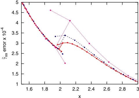
Our particular interest is in the region near the refine-ment interfaces. Figure 4 shows a close-up of~xxnear the refinement boundary at x2M. In this figure we have included the values of the guardcells used for defining finite difference stencils near the interface. Again, the
curves lie nearly atop one another, indicating second order convergence.
A similar close-up of the Hamiltonian constraint H requires a little more explanation. Equation (3a) involves up to second derivatives of the BSSN data, implemented by
-16 -14 -12 -10 -8 -6 -4 -2 0 2
0 0.5 1 1.5 2 2.5 3 3.5 4 4.5 γ∼xx
error x 10
-3 x -16 -14 -12 -10 -8 -6 -4 -2 0 2
0 0.5 1 1.5 2 2.5 3 3.5 4 4.5 γ∼xx
error x 10
-3 x -16 -14 -12 -10 -8 -6 -4 -2 0 2
0 0.5 1 1.5 2 2.5 3 3.5 4 4.5 γ∼xx
error x 10
-3 x -5 0 0 0.2 0 10 20 30 40 50
0 0.5 1 1.5 2 2.5 3 3.5 4 4.5
A
~xx
error x 10
-3 x 0 5 0 0.2 -25 -20 -15 -10 -5 0 5
0 0.5 1 1.5 2 2.5 3 3.5 4 4.5
H error x 10
-3 x -25 -20 -15 -10 -5 0 5
0 0.5 1 1.5 2 2.5 3 3.5 4 4.5
H error x 10
-3 x -25 -20 -15 -10 -5 0 5
0 0.5 1 1.5 2 2.5 3 3.5 4 4.5
H error x 10
-3 x -2 0 0 0.2 -12 -10 -8 -6 -4 -2 0 2
0 0.5 1 1.5 2 2.5 3 3.5 4 4.5
P
x error x 10
-4 x -12 -10 -8 -6 -4 -2 0 2
0 0.5 1 1.5 2 2.5 3 3.5 4 4.5
P
x error x 10
-4 x -12 -10 -8 -6 -4 -2 0 2
0 0.5 1 1.5 2 2.5 3 3.5 4 4.5
P
x error x 10
-4
x -2
0
0 0.2
FIG. 3 (color online). Convergence of the errors (numerical
values minus analytic values) in ~xx, A~xx, the Hamiltonian
constraint H, and the momentum constraintPx, for a
geodesi-cally sliced puncture along thex-axis, all at the timet2:5 M.
The solid line shows the errors for the highest resolution run. The errors for the medium resolution run (dashed line) and the lowest resolution run (dotted line) have been divided by factors of 4 and 16, respectively, to demonstrate second order convergence. Note
that the full domain of the simulation extends to128 M.
1 2 3 4 5 6 7
0 0.5 1 1.5 2 2.5 3 3.5 4 4.5
γ ∼ xx x t=0.5M t=1.0M t=1.5M t=2.0M t=2.5M
FIG. 2 (color online). Evolution of the conformal metric
com-ponent~xx, for a geodesically sliced puncture, shown att0:5,
1.0, 1.5, 2.0, and2:5 M.
1 1.5 2 2.5 3 3.5 4 4.5 5
1.6 1.8 2 2.2 2.4 2.6 2.8 3
γ
∼ xx
error x 10
-4
x
FIG. 4 (color online). Close-up of the convergence of the error
(numerical value minus analytic value) in~xx, for a geodesically
sliced puncture, at t2:5 M, in the vicinity of the refinement
boundary atx2 M. The errors for the high resolution run are
shown by the solid line; the errors for the medium (dashed line) and low (dotted line) resolution runs have been divided by factors of 4 and 16, respectively. In this plot, we also show the location of the data points, including guardcells, using filled circles.
finite differencing. Figure 5 shows the computed values of the Hamiltonian constraint in the vicinity of the refinement boundary at x2M. While the result is second-order convergent at any specific physical point in the neighbor-hood of the boundary, the figure indicates that the sequence of values computed at the nearest point approaching the interface as x!0 approaches zero at only first order. This is as expected according to the discussion in Appendix A (cf. Fig. 12) for a derived quantity involving second derivatives. We have specifically verified that, as with~xx, all BSSN variables converge to second order at the refinement boundaries.
We also examined the simulation data along cuts away from the x-axis and have found them to be qualitatively similar to those on the axis. In particular, plots and anima-tions of the errors along the line yz0:25M can be found in the EPAPS supplement; see Fig. 3(b) and the associated animation file in Ref. [30]. This particular 1-D cut is instructive since it includes the strong-field region yet has no particular symmetric relation to the solution. The fact that the errors along this line are qualitatively similar to those along thex-axis gives us confidence that the results we display in Fig. 3 are not subject to accidental cancella-tions due to octant symmetry boundary condicancella-tions that might produce artificially small errors.
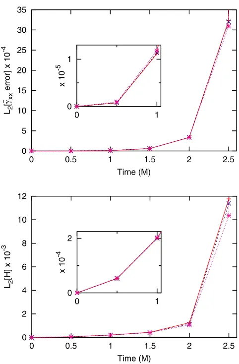
We have also examined the L1 and L2 norms of the errors in basic variables and constraints to assess the over-all properties of the simulation. Representative results are shown in Fig. 6, where the top panel displays the conver-gence behavior of theL2norm of of the error in~xxand the bottom panel the convergence of the L2 norm ofH. The errors for the medium (dashed line) and low (dotted line)
resolution runs have been divided by 4 and 16, respec-tively. These curves lie nearly atop the errors for the high resolution run (solid line), indicating the second order convergence of these error norms; see Appendix C and Eqs. (C3) and (C4).
B.1logslicing
Having rigorously tested the code against an analytic solution, we now use a different coordinate condition to study a longer-lived run with nontrivial, nonlinear dynami-cal behavior in the region of FMR interface boundaries. For this purpose, we again use zero shift but with a modi-fied ‘‘1log’’ slicing condition given by
@
@t 2
4
BLK; (8)
0 5 10 15 20 25 30 35
0 0.5 1 1.5 2 2.5 L2
[
γ
~ xx
error] x 10
-4
Time (M) 0
1
0 1
x 10
-5
0 2 4 6 8 10 12
0 0.5 1 1.5 2 2.5 L2
[H] x 10
-3
Time (M) 0
2
0 1
x 10
-4
FIG. 6 (color online). Convergence of the L2 norms of the
errors in~xxand the Hamiltonian constraintHfor a geodesically
sliced puncture. The numerical data points are here marked with the symbol ‘‘x’’. The solid lines show the errors for the highest resolution run. The errors for the medium resolution run (dashed lines) and the lowest resolution run (dotted lines) have been divided by factors of 4 and 16, respectively, to demonstrate second order convergence.
-2.2 -2 -1.8 -1.6 -1.4 -1.2 -1 -0.8 -0.6 -0.4 -0.2 0 0.2
1.6 1.8 2 2.2 2.4 2.6 2.8 3
H error x 10
-3
x
FIG. 5 (color online). A view of the Hamiltonian constraint in
the neighborhood of the FMR interface atx2 M. The errors
for the high resolution run are shown by the solid line; the errors for the medium (dashed line) and low (dotted line) resolution runs have been divided by factors of 4 and 16, respectively. As discussed in the text, data points nearest to the interface converge at one order lower than in the rest of the domain.
where insertion of the factorBL1M=2r, originally recommended by [18], has proven to enhance convergence near the puncture in our simulations. For the numerical experiments with 1log slicing, the grid structure, in-cluding the locations of the mesh refinement interfaces, is the same as in the geodesic slicing case. We carry out three runs, with low, medium and high resolution defined as before.
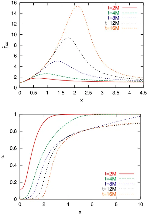
A 1log evolution serves as an excellent numerical experiment to test the robustness of our mesh refinement interfaces. The 1log family has been well-studied in unigrid runs in the past, so the generic behavior of this coordinate system is known and provides a general context for comparison with our mesh refinement results. Because the1logslicing is singularity avoiding, in contrast to the geodesic slicing case, simulations in a1loggauge are known to last30M40M, giving us an opportunity to study the properties of our mesh refinement interfaces in longer duration runs. Finally, as shown by Fig. 7, as the lapse (right panel of the figure) collapses around the
sin-gularity, a strong gradient region in the metric (left panel of the figure) moves outward, passing through mesh refine-ment boundaries in the process. According to unigrid runs already in the literature (e.g., [18]) choosing an appropriate shift, such as the Gamma-driver shift, would cause the evolution to freeze, preventing catastrophic growth in the metric functions and confining the strong field behavior to the region r <10M. This also increases the stable evolu-tion time of the simulaevolu-tions. For our purposes here, how-ever, we choose to let the strong gradient region move outward because we specifically wish to study how well the mesh refinement interfaces handle a strong dynamical potential on timescales t >10M. We consider this an important test, since such phenomena may develop near refinement boundaries in the course of realistic astrophys-ical simulations of multiple black holes.
Having made this choice, we expect to see exactly what appears in Fig. 7. The metric function ~xx (left panel) grows due to well-understood grid stretching related to the collapse of the lapse (right panel) and the fact that grid points are falling into the black hole. The peak of the metric simultaneously moves to larger coordinate po-sition. We expect, therefore, that at some point certain regions of the simulations will no longer exhibit second order convergence because the gradients in the metric simply grow too large, because the peak of the metric moves into a region of lower refinement that cannot resolve the gradients already present in the metric at that point, or because of a combination of the two. The simulations in this gauge, nonetheless, remain second order convergent long enough for us to study the effects of the strong potential passing through the innermost mesh refinement interfaces.
Because we do not have an analytic solution for the
1log case to use in our convergence tests, we show three-point convergence plots instead. Specifically, for a given field f, we plot flowfmed=4 using a dashed line and fmedfhigh using a solid line. Since the three different resolutions ‘‘low’’, ‘‘medium’’, and ‘‘high’’ are related to each other by factors of two, the two lines in each panel should overlay exactly for perfect second order convergence.
Figure 8 shows such a three-point convergence plot for
~
xxandA~xxfor a 1-D cut along thex-axis. The left panels, showing data from t8M, demonstrate that the metric and other variables are second order convergent every-where at that time. Overall, we continue to see second order convergence in the evolved variables, constraints, and norms untilt10M.
The convergent behavior starts to break down around t10Mdue to difficulties with resolving the sharp feature in the metric. In the region 1Mx2M, between the first and second FMR boundaries, the peak itself grows sharply and the coarser grid is not sufficient to provide the resolution needed for convergent behavior. For2Mx
0 2 4 6 8 10 12 14 16
0 0.5 1 1.5 2 2.5 3 3.5 4 4.5
γ
∼ xx
x
t=2M
t=4M t=8M
t=12M
t=16M
0 0.2 0.4 0.6 0.8 1
0 2 4 6 8 10
α
x
t=2M
t=4M t=8M
t=12M
t=16M
FIG. 7 (color online). A time evolution sequence for the
con-formal metric~xx and the lapseusing the variant of1log
slicing given in Eq. (8). Results are shown for the highest resolution run.
4M, the grid is again coarsened by a factor of 2 and is not able to resolve adequately the steep gradient on the leading edge of the metric peak. A snapshot att16Mis shown in the right panels of Fig. 8; by this time, the peak of the metric has passed through two refinement interfaces (at x1M and x2M). The time development of these errors, and, in particular, their departure from second order convergence, can be seen in the animations available in the EPAPS supplement; see Fig. 8(a) and the associated ani-mation file in Ref. [30].
Throughout the duration of the runs the region x*5
does remain second order convergent, even though the grid is further coarsened by factors of two at x8M, 16M,
32M, and64M, since all the fields change very slowly as they approach the asymptotically flat regime. The simula-tions will continue to run stably past this point (to approxi-matelyt 35M), but the resolution in the regions to the right of the interface atx1Mis not sufficient to produce convergent results, as was expected.
The Hamiltonian and momentum constraints along the x-axis are shown in Fig. 9. Three curves are plotted in each panel. The errors for the highest resolution run are given by the solid line. The errors for the medium (dashed line) and low (dotted line) resolution runs have been divided by factors of 4 and 16, respectively. The constraints are second order convergent in the bulk for timest&10M, when the resolution is sufficient to handle the growing feature in the metric (left panels). As expected, H exhibits first order convergent spikes at mesh refinement interfaces;cf.Fig. 5 and Appendix A. Fort*10M, as the peak of the fields propagates into the coarser grid regions pastx2M, the lowest resolutions are not sufficient to resolve the rising slope of the metric, and, like the evolved variables (Fig. 8), the constraints no longer demonstrate second order
con-vergence. The right panels of Fig. 9 show the constraints at t16M, right after the peak of the metric passes through the refinement interface at x2M. See Fig. 9A and the associated animation file in Ref. [30] for animations of these data.
The behavior of the simulations at locations away from the x-axis is qualitatively similar to that shown in Figs. 8 and 9. Plots and animations of the errors along the liney
z0:25M are available in the EPAPS supplement; see Figs. 8(b) and 9(b) and their associated animation files in Ref. [30].
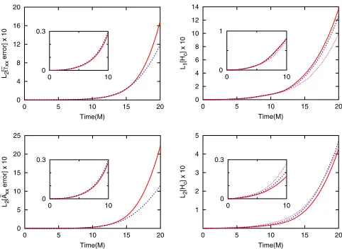
We have also examined the L1 and L2 norms of the errors to assess the overall behavior of these runs, and display representative results in Fig. 10. The L2 norms of the errors in the basic variables ~xxandA~xxare shown in the left top and bottom panels, respectively, using 3-point convergence plots. The dashed lines show the difference between the low and medium resolution results divided by 4, and the solid lines show the difference between the medium and high resolution results, demonstrating the overall second order convergence of these simulations at early times. TheL1norm ofHis displayed in the top right panel, where the solid line gives the errors for the high resolution run. The errors for the medium (dashed line) and low (dotted line) resolution runs have been divided by factors of 4 and 16, respectively, to show second order convergence, as expected from Eq. (C7). In the lower right panel theL2norm ofHis shown, with the solid line giving the results for the high resolution run. As discussed in Appendix C, the errors for the medium (dashed line) and low (dotted line) resolution runs have been divided by factors of 23=2 and43=2 8 to account for the effects of significant first order convergent errors in H at the mesh
-16 -14 -12 -10 -8 -6 -4 -2 0 2
0 0.5 1 1.5 2 2.5 3 3.5 4 4.5
H error x 10
-3
x
-100 -80 -60 -40 -20 0 20
0 0.5 1 1.5 2 2.5 3 3.5 4 4.5
H error x 10
-3
x
-4 -2 0 2 4 6 8
0 0.5 1 1.5 2 2.5 3 3.5 4 4.5
P
x error x 10
-4
x
-20 -15 -10 -5 0 5 10
0 0.5 1 1.5 2 2.5 3 3.5 4 4.5
P
x error x 10
-3
x
FIG. 9 (color online). Convergence plots for the Hamiltonian
constraintHand the momentum constraintPxalong thex-axis in
the 1log slicing runs at times t8 M and t16 M. The
solid lines show the errors for the high resolution run. The errors for the medium (dashed line) and low (dotted line) resolution runs have been divided by factors of 4 and 16, respectively.
-8 -6 -4 -2 0 2 4 6 8 10
0 0.5 1 1.5 2 2.5 3 3.5 4 4.5
γ
~xx
error x 10
-3
x
-4 -3 -2 -1 0 1 2 3
0 0.5 1 1.5 2 2.5 3 3.5 4 4.5
γ
~xx
error x 10
x
-10 -5 0 5 10 15 20 25
0 0.5 1 1.5 2 2.5 3 3.5 4 4.5
A
~ xx
error x 10
-3
x
-4 -3 -2 -1 0 1 2 3 4 5 6 7
0 0.5 1 1.5 2 2.5 3 3.5 4 4.5
A
~ xx
error x 10
x
FIG. 8 (color online). Three-point convergence plots for the
BSSN variables ~xx and A~xx along the x-axis in the 1log
slicing runs at timest8 M(left panels) andt16 M(right
panels). For a given field f, the dashed line shows flow
fmed=4and the solid line showsfmedfhigh.
refinement boundaries, in addition to the second order convergent errors in the bulk; see Eq. (C8).
One final feature of these simulations, the high fre-quency noise near the origin seen in the right panels of Fig. 9, requires some explanation. First of all, it is not related to the presence of the refinement boundaries; in particular, we have reproduced it in unigrid runs and with an independently-written, 1-D (spherically symmetric) code. Higher resolution exacerbates this problem: both the frequency and amplitude of the noise increase with resolution. We have found the location of this noise to be independent of resolution and the number and positions of FMR boundaries.
This feature, which we call the ‘‘point-twoMproblem,’’ originates around r0:2M. It becomes most evident at timest >10M, first appearing in the lapse andK, which are directly coupled, and then eventually mixing into all of the extrinsic curvature variables. For the duration of the evolutions the noise remains within the region 0:0M&
x&0:5M. Outside this region, all basic variables demon-strate satisfactory second order convergence, including at refinement boundaries, up to timest10M.
Having chosen a generally accepted gauge, and having focused on effects of the mesh refinement interfaces in this work, we have not fully investigated the cause of
nor possible remedies for this apparent pathology. We note it here, however, as an interesting topic for future investigation.
V. SUMMARY
This paper demonstrates that fixed mesh refinement boundaries can be located in the strong-field regionof a dynamical black hole spacetime when the interface con-ditions are handled properly. This result was verified through simulation of a Schwarzschild black hole in geo-desic coordinates, for which we have an analytic solution for comparision, and through simulations of Schwarzschild in a variation of the1log(singularity avoiding) slicing with zero shift. Mesh refinement technology, therefore, is a viable to way to use computational resources more effi-ciently, and to simulate the very large spatial domains needed to compute the dynamics of the source interactions and allow extraction of the resulting gravitational waveforms.
Our method for handling the interface conditions, based in part on the Paramesh infrastructure, is detailed. For these simulations we find that, in handling the interface condi-tion between FMR levels, third order guard cell filling is sufficient for overall second order accuracy in the simula-tions. By nesting several levels of mesh refinement regions, we are able to resolve the puncture convergently while simultaneously pushing the outer boundary of our domain to 128M and keeping the computational problem size modest. We estimate that for only a 12% increase in the computational size of the problem, we could push the outer boundary to 256M; moving the outer boundary out even farther will be possible for production runs on larger machines. Combined with our earlier results showing that gravitational waves pass through such FMR interfaces without significant reflections [14], we have now studied, in detail, the effects of FMR interfaces on the two primary features, waves and time-varying strong potentials, of as-trophysically interesting spacetimes.
In this paper, we have evolved single black holes using gauges with zero shift in order to produce test problems in which strong-field spacetime features with steep gradients pass through mesh refinement interfaces. In more realistic, astrophysical simulations of multiple black holes, we ex-pect to use nonzero shift prescriptions. While a shift vector will allow us to control certain aspects of the dynamics, we still expect to find some strong, time-varying signals to propagate across mesh refinement boundaries. We are currently implementing nonzero shift conditions into our FMR evolutions and will report on this work in a separate publication.
ACKNOWLEDGMENTS
It is a pleasure to thank Richard Matzner for his pene-trating discussions about convergence of code results, 0
4 8 12 16 20
0 5 10 15 20
L2
[
γ
~ xx
error] x 10
Time(M) 0
0.3
0 10
0 2 4 6 8 10 12 14
0 5 10 15 20
L1 [Hc
] x 10
Time(M) 0
1
0 10
0 5 10 15 20 25
0 5 10 15 20
L2
[A
~ xx
error] x 10
Time(M) 0
0.3
0 10
1 2 3 4 5
0 5 10 15 20
L2
[H
c
] x 10
Time(M) 0
0.3
0 10
FIG. 10 (color online). Convergence behavior of theL1andL2
norms of the errors for the runs with1log slicing. The left
panel shows the L2 norms of the errors in ~xx (top) and A~xx
(bottom), where the dashed lines show the the difference be-tween the low and medium resolution results divided by 4, and the solid lines show the difference between the medium and high
resolution results. The top right panel shows theL1norm ofH,
with the solid line giving the errors for the high resolution run; the errors for the medium (dashed line) and low (dotted line) resolution runs have been divided by factors of 4 and 16,
respectively. The lower right panel shows the L2 norm of H,
with the solid line giving the results for the high resolution run. In this panel, the errors for the medium (dashed line) and low
(dotted line) resolution runs have been divided by factors of23=2
and43=28, respectively.
and Peter MacNeice for his enlightening replies to our queries about Paramesh and other code related issues. We are also grateful to Josephine Palencia and Jeff Simpson, who provided essential computer support during the course of this investigation. This research was supported in part by NASA Space Sciences grant ATP02-0043-0056. The work of J. B. and J. v. M. was supported in part by the National Research Council at the Goddard Space Flight Center. J. D. B. also received funding from NSF grant PHY– 0070892. The computations were carried out on Beowulf clusters operated by the Space Science Data Operations Office and the Commodity Cluster Computing Group at Goddard.
APPENDIX A: ERROR ANALYSIS OF GUARD CELL FILLING SCHEME
To help pave the way for understanding the behavior of our black hole evolutions near mesh refinement bounda-ries, we provide here a detailed analysis of a toy model for a scalar field in one spatial dimension, using the same third order guard cell filling algorithm detailed in Sec. III. The model equations are
_ $ (A1a)
_
$ 00; (A1b)
where the dot denotes a time derivative and primes denote space derivatives. These equations can be solved numeri-cally using the same twice-iterated Crank-Nicholson algo-rithm used to evolve our black hole spacetimes. The fields at timestepn1are given in terms of the fields at timestep nby
n1
j njt$nj
t2
2 D
2 n j
t3
4 D
2$n
j (A2a)
$n1
j $njtD2 nj
t2
2 D
2$n j
t3
4 D
4 n
j (A2b)
whereD2is a finite difference operator approximating the second spatial derivative, andD4 D22.
Consider for the moment a uniform spatial grid. IfD2is the usual second order accurate centered difference opera-tor, the dominant source of error for n1
j comes from the term proportional tot3. This term has the wrong numeri-cal coefficient as compared to the Taylor series expansion of the exact solution. The dominant sources of error for $n1
j come from the term proportional tot3, which also has the wrong numerical coefficient, and from the second order error inD2 n
j. For a uniform grid the dominant error inD2 n
j isD4 jnx2=12, so the leading errors for a single timestep are
n1
j err
1
12t
3D2$n
j (A3a)
$n1 j err
1
12tt
2x2D4 n
j: (A3b)
Fortx, each of these one-time-step errors is propor-tional tox3. If we evolve the initial data to a finite timeT, the Ox3 errors accumulate over NT=t timesteps resulting in second order errors.4Thus, the basic variables and$are second order convergent on a uniform grid. On a nonuniform grid, guard cell filling introduces errors of order x3 in at grid points adjacent to the boundary. This leads to errors of order xin D2 n
j and
1=xinD4 nj. From Eq. (A2b) we see that in one timestep $can acquire errors of orderx2. The concern is that these errors might accumulate overNT=ttimesteps to yield first order errors. This, in fact, does not happen. Simple numerical experiments show that and$are second order convergent on a nonuniform grid with third order guard cell filling.
We can understand this result with the following heu-ristic reasoning. The numerical algorithm of Eq. (A2) ap-proximates, as does any mathematically sound numerical scheme, the exact solution of the scalar field equations (Eq. (A1)) in which the field$propagates along the light cone. The ‘‘bulk’’ errors displayed in Eq. (A3b) accumu-late along the past light cone to produce an overall error of orderNx3x2at each spacetime point. Errors in guard cell filling, which occur at a fixed spatial location, do not accumulate over multiple timesteps since the past light cone of a given spacetime point will cross the interface (typically) no more than once.
The characteristic fields for the system (A1) are$ 0 so that 0, like $, propagates along the light cone. As a result, the value of at a given spacetime point is deter-mined by data from theinteriorof the past light cone. From Eq. (A2a) we see that the one-time-step errors for due to guard cell filling are orderx3. These errors can accumu-late overNtimesteps to yield errors of orderNx3x2. The derivatives 0 and 00are computed at finite timeT by evolving the , $ system for T=t timesteps then taking the centered, second order accurate numerical de-rivatives of . Numerical experiments show that 0and 00, defined in this way, are second order convergent on a non-uniform grid with third order guard cell filling.5 Continuing with our heuristic discussion, we can under-stand the second order convergence of 00 as follows. Let
n
jerr Enjx2 denote the error in at grid pointn, j, where the coefficientEn
jis independent ofx. Some of this error is due to guard cell filling at the mesh refinement interface and some is due to the accumulation of bulk errors (A3). Now, the second derivative of , computed asD2 n
j nj12 nj nj1=x2, will contain errors
4This is a simplification. The dominant error afterNtimesteps
includes other terms of orderx2in addition to the product ofN
and the one-time-step error. These other terms include, for
example, the product of an order N3 coefficient and a
one-time-step error of orderx5.
5The error in 00 is fairly noisy but the overall envelope
containing this noise is second order convergent.
of the form D2 n
jerr Enj12Enj Enj1. Since the bulk errors are smooth, the bulk contribution to En
j1
2En
jEnj1 will scale asx2. It is also the case that the errors due to guard cell filling are smooth. This is because the value of at any given point is determined by the interior of the past light cone, so its error includes an accumulation of guard cell filling errors along the history of the mesh refinement interface. In the limit of high resolution this accumulation of error approaches the same value at neighboring grid points j1, j, and j1. In other words, the guard cell filling contribution to En
j12Enj Enj1 approaches zero as x!0. Evidently, the guard cell filling contribution, like the bulk contribution, scales likex2.
The discussion above indicates that we can evolve the scalar field system of Eq. (A1) for a finite time on a grid with mesh refinement, numerically compute the second derivative of , and find that 00 is second order accurate. Without shift, the BSSN Eqs. (2c) and (2d) are similar to the scalar field equations with~ijplaying the role of and
A~
ij playing the role of $. This feature was one of the original motivations behind the BSSN system. Note that the term analogous to 00 in the $_ equation is the term
~
lm~ij;lm contained in the trace-free part of the Ricci tensor, which appears on the right-hand side of Eq. (2d). Obviously there are many other terms that appear on the right-hand side of thedA~ij=dtequation. We can model the effect of these terms by including a fixed function on the right-hand side of the$_ equation:
_ $ (A4a)
_
$ 00-00: (A4b)
We have written the fixed function as the second derivative of-. For simplicity we choose-to depend onxonly, the most relevant dependence for our consideration of behav-ior across spatial resolution interfaces. The general solu-tion of this system is then
t; x t; x -x (A5a)
$t; x $t; x (A5b)
where ,$ is a solution of the homogeneous wave equa-tion (Eq. (A1)).
The extended model system of Eq. (A4) can be solved numerically with the discretization
n1
j jnt$nj . . . (A6a)
$n1
j $nj tD2 njD2-j . . . (A6b)
The higher order terms int, not shown here, come from the iterations in our iterated Crank-Nicholson algorithm. It is important to recognize that the-00 term is expressed as the numerical second derivative of-j and not as the dis-cretization of the analytical second derivative,-00j. The reason for this choice is thatD2-jmimics the effect of the
extra terms on the right-hand side of Eq. (2d) which, in our BSSN code, depend on the discrete first and second de-rivatives of the BSSN variablesand~i.
From the discussion of the wave equation (Eq. (A1)) we can anticipate the results of numerical experiments with the model system (Eq. (A4)) on a non-uniform grid. For arbitrary initial data 0
j,$0j, the numerical solution is given by
n
j nj -j (A7a)
$n
j $nj (A7b)
where n
j,$nj is the numerical solution of the homogene-ous wave equation (Eq. (A1)) with initial data 0j-j,$0j. The order of convergence for n
j is determined by how rapidly, as x!0, the numerical solution in Eq. (A7a) approaches the exact solution t; x t; x -x. Since -jis simply the projection of the analytic function -xonto the numerical grid, the term-jin the numerical solution (Eq. (A7a)) does not contribute any error. We have already determined that on a non-uniform grid n
j ap-proaches t; x with second order accuracy. Thus, we expect n
j to be second order convergent.
What about derivatives of ? The order of convergence for D1 n
j is found by comparing the discrete derivative D1 nj D1 njD1-jto the analytic solution 0 0 -0. Again, as we have discussed,D1 n
japproaches 0with second order errors. It is also easy to see that the numerical derivativeD1
-japproaches-0with second order accuracy. Away from grid interfaces this is obviously true, assuming that D1 is the standard second order accurate centered difference operator. For points adjacent to a grid interface, guard cell values for are filled with third order errors. These errors lead to second order errors in D1 n
j. Overall then, we expect second order convergence forD1 n
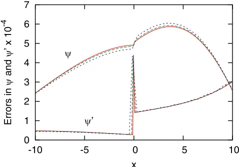
j. The expected convergence rates for and 0 are con-firmed by the results shown in Fig. 11. For these numerical tests, we chose-x expx50=10and initial data
0; x 100ex102=400
ex50=10 (A8a)
$0; x 1
2x10e
x102=400
: (A8b)
Each set of curves shows the errors at three different resolutions,x5=16,5=32, and 5=64, wherexis the fine grid spacing. The evolution time is20:83, correspond-ing to200,400, or800timesteps (depending on the reso-lution) and a Courant factor of1=3.
The order of convergence for the second derivative of is determined from a comparison of D2 n
j D2 nj D2
-j and the analytic solution 00 00-00. We have seen thatD2 n
japproaches 00with second order accuracy. The situation for D2
-j, however, is somewhat different. Away from any grid interfaceD2-jwill approach-00with
second order accuracy, assumingD2is the standard second order accurate finite difference operator. But for points adjacent to the interface, and only those points, guard cell filling errors of orderx3 in-will lead to first order errors in D2
-j. Thus, we expect to find second order convergence for D2 n
j at all points except those points adjacent to the interface. Points adjacent to the interface should be first order convergent.
Figure 12 shows the results of our convergence test for 00. The spikes at the interface (x0) appear because the two grid points adjacent to the interface are only first order convergent. Elsewhere, the plot shows second order convergence.
The behavior demonstrated in Fig. 12 also occurs in the BSSN system when we examine the convergence plot for the Hamiltonian constraint. In graphing the Hamiltonian constraint H, we are comparing a combination of grid functions that includes second derivatives of the BSSN variables to the exact analytical solution for H, namely, zero. We therefore expect spikes to appear at interfaces in the convergence plot for the Hamiltonian constraint, and indeed they do (see, for example, Figs. 3 and 9 ).
We wish to emphasize that the lack of second order convergence for second spatial derivatives at grid points adjacent to the interfaces is not due to any error in our code, or shortcoming of the numerical algorithm. Since the un-differentiated variables are second order convergent every-where, we can always assure second order convergence of their derivatives by using suitable finite difference stencils. For example, in computing D2 nj from n
j we can use a second order accurate one-sided operator D2 that avoids using guard cell values altogether. With such a choice the spikes in Fig. 12 disappear, andD2 nj is everywhere
sec-ond order convergent. In our BSSN code, it is most con-venient to compute the Hamiltonian constraint using the same centered difference operator D2 that we use for the evolution equations. As a consequence, spikes appear at the grid interfaces in the convergence plots (Fig. 3 and 9).
APPENDIX B: ANALYTIC SOLUTION FOR GEODESICALLY SLICED SCHWARZSCHILD
In a numerical simulation, geodesic coordinates are obtained by using unit lapse and vanishing shift. This implies that the grid points will follow geodesic trajectories through the physical spacetime. We present here a physical derivation of the Schwarzchild spacetime metric in this well-known coordinate system, based on those geodesics; an alternate derivation is available in Refs. [6,7,31].
The Schwarzschild geometry in standard coordinates is given by
ds2 g
TTdT2gRRdR2R2d!2; (B1)
wheregTT g1RR 12M=R.
To express this metric in geodesic coordinates, consider a spatial Cauchy surface 0 in a 4-manifold M and a congruence of radial geodesics crossing0. Let the affine parameter&for each geodesic be zero at0. Considering subsequent slices of constant proper time, we can set a global time&which we use to define a new foliation&of
M. Each geodesic in the congruence is labeled by the coordinates of its initial ‘‘starting’’ point in0. The radial position/of the starting point in0can thus be promoted to a new radial coordinate on M to pair with the time coordinate&.
0 1 2 3 4 5 6 7
-10 -5 0 5 10
Errors in
ψ
and
ψ
’ x 10
-4
x ψ
ψ’
FIG. 11 (color online). Convergence tests for and 0. The
mesh interface is at x0, with the fine grid on the left and
coarse grid on the right. The errors in and 0 for the high
resolution case are shown by the solid line. The errors are divided by factors of 4 and 16 for the middle (dashed line) and low (dotted line) resolution cases, respectively.
-2 -1 0 1 2 3 4 5 6
-2 -1.5 -1 -0.5 0 0.5 1 1.5 2
Error in
ψ
’’ x 10
-3
x
FIG. 12 (color online). Convergence test for 00. The solid
curve is the error in 00 for the highest resolution run. As in
Fig. 11, the interface is at x0 and the errors for the middle
(dashed line) and low (dotted line) resolution cases are divided by factors of 4 and 16, respectively. The grid points adjacent to
the interface do not coincide because 00 is only first order
convergent at these points.