Evaluation of Variability in the Assessment of Small Color Differences

Abstract

CÁRDENAS, LINA MARIA. Evaluation of Variability in Visual Assessment of Small Color Differences. (Under the direction of Drs. Renzo Shamey and David Hinks).

Several psychophysical methods and the associated intra and inter-observer variability in assessing small color differences of textile samples were investigated in three phases:

• Development and validation of a novel perceptually linear gray scale and incorporation into a visual assessment protocol;

• Development and determination of a robust visual assessment protocol via testing different psychophysical methods and viewing conditions;

• International replication experiment employing a controlled methodology to assess the repeatability of results and ascertain the degree of variability among observer panels from four continents.

During the second phase, five visual assessment methodologies: AATCC standard gray scale, Jumbo scale, Jumbo scale with gap, novel perceptually linear scale, as well as pair comparison were evaluated to determine the method generating the lowest intra- and inter-observer variation. Thirty one polyester knitted samples around 13 color centers were assessed by panels of 25 observers. The visual assessment based on the use of the Jumbo scale, on average, produced the largest visual color differences for all pairs, whereas the assessments based on the standard AATCC scale produced the lowest visual color difference. A comparison of visual data obtained from different methods based on the STRESS function showed that various methodologies produced comparable visual data. However, intra- and inter-observer variability significantly decreased when the perceptually linear gray scale was employed relative to when any of the geometric scales were used.

A highly controlled replication study was carried out to test, systematically and for the first time, the range and magnitude of variability among four panels of observers from different regions of the world: Colombia, Czech Republic, USA, and a group of Chinese born and raised observers. Sixty nine polyester knitted samples around 13 color centers were assessed by 25 observers in each location using the same method.

degree of variation (intra-group standard deviation) among responses from any panel compared to the mean response of that panel was not significantly different amongst panels.

The performance of color difference equations was tested against the average visual data for each of the observer panels as well as the combined dataset using PF/3 and STRESS functions. Results showed that the ΔE*ab equation performed significantly poorer than

CMC(1:1) and CIEDE2000(1:1:1) models. In addition the STRESS function showed no

significant difference between CMC(1:1) and CIEDE2000(1:1:1) models for the visual data

Evaluation of Variability in Visual Assessment of Small Color Differences

by

Lina María Cárdenas

A dissertation submitted to the Graduate Faculty of North Carolina State University

In partial fulfillment of the Requirements for the degree of

Doctor of Philosophy

Fiber and Polymer Science

Raleigh, North Carolina February 24th, 2009

APPROVED BY:

_______________________________ ______________________________

Dr. Renzo Shamey Dr. David Hinks

Committee Co-chair Committee Co-chair

________________________________ ________________________________

ii

Dedication

iii

Biography

Lina María Cárdenas was born in Sogamoso, Colombia, in 1979. She received her B.S in Textile Design from Universidad de los Andes, Bogotá, Colombia in 2002, and conducted

her undergraduate research on rabbit hair felt used in the production of hats.

iv

Acknowledgements

The author would like to thank Drs. Renzo Shamey and David Hinks, chairman and co-chairman of her advisory committee, for their advice, support, patience, and guidance throughout this research; Dr. Roger Woodard, member of the advisory committee, for the great contribution to the author’s understanding, development, and interpretation of the statistical analysis. Their continuous encouragement and enthusiasm made an incredible difference for the author. Also, I would like to extend my gratitude to Dr. Warren Jasper, member of the advisory committee, for his valuable suggestions and encouragement. The author would also like to thank Prof. Rolf Kuehni for his invaluable ideas and comments.

Special thanks go to the National Textile Center, USA, for financial support of this project, without which this project would not have been possible.

v Also, I would like to thank Dr. Maria Oliver-Hoyo, Ms. Laleh Shamey, Miss Li Liu, and Mr. Gang Fang for helping the author recruit Chinese observers.

The author is very grateful for the special paint developments made by the staff of Porter Paints at the Raleigh’s office for the development of the perceptual linear gray scale.

The author would also like to thank all observers who participated in the visual assessments and those who collaborated in one way or another with the success of this study

A special thanks to Mr. John Darsey and colleagues at DyStar for generation of the dyed fabric samples.

vi

Table of Contents

List of Figures……….xii

List of Tables………..xvi

I. Introduction ... 1

1. Research Proposal ... 7

1.1. Objectives ... 7

II. Literature Review ... 9

1. Human Color Vision ... 9

1.1. The Eye ... 9

1.1.1. The Sclera ... 10

1.1.2. The Cornea ... 10

1.1.3. The Iris ... 11

1.1.4. The Lens ... 11

1.1.5. The Humors ... 12

1.1.6. The Retina ... 12

1.1.7. The Fovea and Macula ... 13

1.2. The Eye and the Brain: How Color Vision Experience is Produced ... 14

1.2.1. Receptive Fields ... 17

1.2.2. Rods and Cones ... 18

1.2.3. Monochrome Vision ... 20

1.2.4. Color Vision ... 20

1.3. Mechanisms of Color Vision ... 21

1.3.1. Trichromatic Theory ... 21

1.3.2. Hering’s Opponent – Color Theory ... 21

1.3.3. Recent Developments in Color Vision Mechanisms ... 22

1.4. Mechanisms of Adaptation ... 23

1.4.1. Dark Adaptation ... 23

1.4.2. Light Adaptation ... 24

1.4.3. Chromatic Adaptation ... 24

1.4.4. Visual Mechanisms Affecting Color Perception ... 25

1.5. Color Vision Deficiencies ... 25

1.5.1. Inherited Color Vision Deficiency ... 26

1.5.2. Acquired Color Vision Deficiency ... 29

1.6. Color Testing Methods ... 31

1.6.1. Ishihara test ... 31

1.6.2. Farnsworth –Munsell 100-Hue Test ... 32

vii

1.6.4. Cambridge Color Test (CCT) ... 33

1.6.5. Color Vision Test Made Easy ... 33

2. Psychophysics ... 34

2.1. Definition ... 34

2.2. Historical Overview ... 34

2.3. Detection Techniques ... 36

2.3.1. Method of Adjustment ... 36

2.3.2. Method of Limits ... 37

2.3.3. Method of Constant Stimuli ... 37

2.4. Matching Techniques ... 38

2.4.1. Asymmetric Matching ... 39

2.4.2. Memory Matching ... 39

2.5. Scaling Methods... 39

2.5.1. Types of Scales ... 40

2.6. One Dimensional Scaling ... 41

2.6.1. Rank Order ... 41

2.6.2. Graphical Rating ... 42

2.6.3. Category Scaling ... 42

2.6.4. Paired Comparisons ... 42

2.7. Techniques Used In Color Research ... 43

2.7.1. Studies Comparing Psychophysical Techniques ... 43

2.7.2. Studies Using Gray Scale Method for Perceptibility Studies ... 45

2.7.3. Studies Using Pair Comparison Method for Perceptibility Studies ... 46

2.7.4. Other Psychophysical Methods ... 47

2.7.5. Methodologies Recommended for Selection and Training in Color Assessment 47 2.7.6. Methodology Recommended for Visual Assessment of Color Difference ... 48

3. Colorimetry ... 49

3.1. Color ... 50

3.1.1. Illuminants and Light Sources ... 51

3.1.2. Colored Object ... 58

3.2. Tristimulus Values and Color Matching Functions ... 60

3.2.1. The 1931 CIE Standard Observer ... 60

3.2.2. The 1964 CIE Standard Observer ... 64

3.2.3. Calculating Tristimulus Values ... 65

3.3. Chromaticity Diagrams ... 67

3.4. Measuring Color ... 70

3.4.1. Visual Assessment ... 70

3.4.2. Instrumental Measurement ... 71

3.4.3. Summary ... 79

viii

4.1. Important Definitions ... 81

4.1.1. Hue ... 81

4.1.2. Lightness ... 82

4.1.3. Chroma ... 84

4.1.4. Unrelated and Related Colors ... 85

4.2. Additional Perceptual Phenomena ... 85

4.2.1. Simultaneous Contrast or Chromatic Induction ... 85

4.2.2. Successive Contrast (Afterimage Effect) ... 87

4.2.3. Spreading ... 88

4.2.4. Mach Bands ... 89

4.2.5. Color Constancy ... 90

4.2.6. Metamerism ... 92

5. Color Specification ... 97

5.1. Color Order Systems ... 97

5.1.1. Systems Based on Color Perception ... 97

5.2. Color Spaces ... 102

5.2.1. CIE xyY ... 102

5.2.2. Judd and MacAdam UCS (Uniform-Chromaticity Scale) Diagrams ... 103

5.2.3. Hunter Lαβ and Scofield Lab Color Spaces ... 104

5.2.4. Adams Chromatic Value Color Space ... 104

5.2.5. Hunter Lab Color Space ... 105

5.2.6. Adams-Nickerson (ANLAB) Color Space ... 106

5.2.7. CIE 1960 UCS Diagram and CIE 1964 (U*V*W*) Color Space ... 107

5.2.8. CIE 1976 UCS Diagram ... 107

5.2.9. CIELUV Color Space ... 108

5.2.10. CIELAB Color Space ... 109

5.3. Color Difference Formulas ... 112

5.3.1. Tolerance ... 113

5.3.2. CIELAB and CIELUV Color Difference Formula ... 114

5.3.3. JPC79 Color Difference Formula ... 116

5.3.4. CMC (l:c) Color Difference Formula ... 117

5.3.5. BFD (l:c) Color Difference Formula ... 119

5.3.6. CIE94 (KL:KC:KH) Color Difference Formula... 120

5.3.7. CIEDE2000 (KL: KC: KH) Color Difference Formula ... 121

5.3.8. Performance of Color Difference Equations ... 123

6. Statistical Methods for Evaluating Color Difference Formulas and Color Difference Assessments ... 125

6.1. Statistical Methods Used in Color Difference Evaluation ... 125

6.1.1. Correlation Coefficient ... 125

ix

6.1.3. Performance Factor (PF/4 and PF/3) ... 126

6.1.4. VM Index ... 129

6.1.5. Standardized Residual Sum of Squares (STRESS) ... 131

6.2. Regular Statistical Methods used for Analysis of Variance ... 133

6.2.1. Paired t-test ... 133

6.2.2. Measurement Errors ... 134

6.2.3. Estimating Measurement Error ... 135

III. Experimental Methodology and Determination of Parameters Affecting Visual Assessments ... 141

1. Introduction ... 141

2. Assessment of the Type of Observer: Comparison of Naïve and Expert Observers in the Assessment of Small Color Differences ... 144

2.1. Experimental ... 145

2.1.1. Samples ... 145

2.1.2. Sample Viewing ... 147

2.1.3. Psychophysical Method ... 149

2.2. Analysis of Data ... 150

2.2.1. Gray Scale Transformations to Visual Difference ... 150

2.2.2. Comparing Performance of Naïve and Expert Assessors ... 151

2.2.3. Analysis of Variance ... 151

2.2.4. Intra-Observer Variability ... 157

2.3. Results and Discussion ... 158

2.3.1. Systematic Errors: Intra-Group Variation (Observer Accuracy) ... 161

2.3.2. Random Errors: Variance Component Analysis ... 162

2.3.3. Intra-Observer Variability (Observer Consistency) ... 165

2.3.4. Observer Accuracy using PF/3 Metric ... 166

2.3.5. PF/3 Observer Repeatability (Observer Consistency) ... 168

2.3.6. Performance of Color Difference Formulas against each Visual Dataset ... 170

2.3.7. Performance of Color Difference Formulas against each Visual Dataset using the STRESS Function ... 171

2.4. Conclusions ... 174

3. Effect of Variables on Visual Assessment of Small Color Differences ... 177

3.1. Visual Assessment using Pair Comparison Method ... 177

3.1.1. Experimental ... 178

3.1.2. Analysis of Data ... 180

3.1.3. Results and Discussion ... 183

3.1.4. Conclusions ... 190

3.2. Visual Assessment Using a Jumbo Gray Scale ... 192

3.2.1. Experimental ... 192

x

3.2.3. Results and Discussion ... 196

3.2.4. Conclusions ... 207

3.3. Visual Assessment Using Jumbo Scale with Gap ... 210

3.3.1. Experimental ... 210

3.3.2. Analysis of Data ... 213

3.3.3. Results and Discussion ... 214

3.3.4. Conclusions ... 226

4. Development of a Linear Gray Scale for Visual Assessment of Small Color Differences ... 228

4.1. Development of a Perceptually Linear Gray Scale ... 233

4.1.1. Experimental ... 234

4.1.2. Data Analysis ... 241

4.1.3. Conclusions ... 245

4.2. Validation of the Perceptually Linear Scale ... 247

4.3. Visual Assessment of Small Color Differences Using a Novel Perceptually Linear Gray Scale ... 249

4.3.1. Experimental ... 249

4.3.2. Data Analysis ... 253

4.3.3. Results and Discussion ... 254

4.3.4. Conclusions ... 264

5. Comparison of Various Psychophysical Methods ... 267

5.1. Average Perceived Color Difference Using Different Experimental Methods ... 269

5.2. Intra-Group Variability ... 272

5.3. Intra-Observer Variability ... 273

5.4. Variance Component Analysis ... 275

5.5. PF/3 Accuracy and PF/3 Repeatability ... 276

5.5.1. Correlation between PF/3 Accuracy and PF/3 Repeatability... 278

5.6. PF/3 of Agreement among Visual Results from Different Methodologies ... 279

5.7. Performance of Existing Color Difference Models Using PF/3 Metric ... 280

5.8. Performance of Color Difference Models Using STRESS ... 281

5.9. Conclusions ... 282

IV. Inter and Intra-Observer Variability in an Internationally Replicated Study of Assessing Small Color Differences among Textile Samples ... 287

1. Experimental ... 289

1.1. Samples ... 289

1.2. Sample Viewing ... 291

1.3. Psychophysical Method ... 291

2. Data Analysis ... 295

2.1. Gray Scale Transformations to Visual Difference ... 295

xi

3. Results and Discussion ... 296

3.1. Variance of Pairs ... 296

3.2. Systematic Errors ... 297

3.2.1. Intra-group variation (Observer Accuracy)... 297

3.3. Random Errors ... 299

3.3.1. Variance Component Analysis... 299

3.4. Intra-Observer Variability (Observer Consistency) ... 301

3.5. Observer Accuracy using PF/3 Metric ... 303

3.6. PF/3 Observer Repeatability ... 306

3.7. Performance of Color Difference Formulas against Visual Datasets from each Observer Panel ... 307

3.8. PF/3 of Agreement among Visual Results from Different Observer Panels ... 310

3.9. Performance of Color Difference Formulas against Each Visual Dataset using STRESS ... 311

3.10. Confidence intervals for each pair for the observers panels ... 314

3.11. Confidence Intervals for each Pair for all the Observers’ Panels Combined ... 319

3.12. Performance of Color Difference Formulas against Visual Datasets from all observers’ panels ... 321

3.13. Performance of Color Difference Formulas against the grand mean visual from all observer panels using STRESS ... 323

4. Conclusions ... 326

V. Summary of Conclusions ... 332

1. Role of Observer: Expert vs. Naïve Observers ... 332

2. Development of a Linear Gray Scale for Visual Assessment of Small Color Differences ... 333

3. Observer Variability in Small Color Difference Assessments Using Various Psychophysical Methods ... 334

3.1. Pair Comparison Method ... 334

3.2. Gray Scale Methods ... 334

3.2.1. Type of Scale: Standard Geometric Scale (AATCC) vs. Novel Perceptually Linear Scale ... 335

3.2.2. Size of Scale: Standard AATCC Geometric Scale vs. Jumbo Gray Scale ... 336

3.2.3. Sample Separation: Jumbo Gray Scale vs. Jumbo Gray Scale with Gap ... 337

4. Replication Experiment ... 339

4.1. Performance of Existing Models Based on Results of Replication Study ... 340

VI. Future Work ... 342

VII. References ... 346

xii

List of Figures

Figure 1. Key variables in the control of color in the supply chain. ... 3

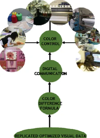
Figure 2. Flowchart of steps required for optimization of color control in the textile supply chain. ... 4

Figure 3. Human eye and its principal parts. ... 10

Figure 4. Shape of rods and cones. ... 13

Figure 5. Optic axis. ... 14

Figure 6. Cross-section of the retina. ... 15

Figure 7. Diagram of the visual pathway to the LGN. ... 16

Figure 8. Receptive fields from a ganglion cell ((a)on-center, (b) off-center). ... 17

Figure 9. Dark adaptation recovery. ... 24

Figure 10. (a) Normal vision (b) protanope (c) deuteranope (d) tritanope. ... 28

Figure 11. Percentages of Incidence of defective color vision around de world. ... 29

Figure 12. Ishiara plate. ... 32

Figure 13. Sample arrangement used in a pair comparison experiment. ... 44

Figure 14. Sample arrangement used in a gray scale experiment. ... 44

Figure 15. The three basic components needed for color perception. ... 50

Figure 16. The visible spectrum in relationship to other types of electromagnetic radiation. 52 Figure 17. Spectral power distribution of CIE standard illuminants (a) Illuminant A (b) Illuminants F2 and F11 (c) Illuminants C, D50, D65. ... 57

Figure 18. Color matching functions for the 1931 standard observer. ... 62

Figure 19. 1931 Standard observer. ... 63

Figure 20. (a) 1931 x,y chromaticity diagram (b) u’v’ uniform-chromaticity scale diagram. 69 Figure 21. Scheme of a colorimeter. ... 72

Figure 22. Diagram of a dual beam spectrophotometer. ... 74

Figure 23. Most commonly used viewing geometries: a) 0/45 b) 45/0 c) 0/ diffused d) Diffuse/0. ... 75

Figure 24. Colored squares at high saturation surrounded by gray square with the same lightness values (Helmontz-Kohlrausch effect). ... 83

Figure 25. Lightness crispening effect. ... 84

Figure 26. Simultaneous contrast. ... 86

Figure 27. Simultaneous contrast in pairs. ... 86

Figure 28. Afterimage effect. ... 88

Figure 29. Spreading effect. ... 89

Figure 30. Mach bands. ... 90

Figure 31. Metamerism Effect. ... 92

Figure 32. Reflectance curves for a metameric pair. ... 93

xiii

Figure 34. Natural Color System. ... 100

Figure 35. Structure of the OSA Uniform Color Scales System. ... 101

Figure 36. CIE xyY color space. ... 103

Figure 37. Representation of the CIELAB Coordinates. ... 110

Figure 38. Schematic non-uniformity of the CIELAB color space. ... 111

Figure 39. Location of dyed samples in the CIE a*b* plane. ... 145

Figure 40. Appearance of color standards used for visual assessments. ... 146

Figure 41.The experimental set up for visual assessment of color difference using an AATCC gray scale. ... 148

Figure 42. Graph of ΔV for the visual assessments of each sample pair, ranked in ascending order of ΔE*ab. ... 158

Figure 43. Comparison of the performance of individual observers in terms of PF/3 repeatability among trials. ... 170

Figure 44. Graph of PF/3 for ΔE*ab, CMC(1:1), and CIEDE2000 (1:1:1) for the average naïve observers (three trials) and expert observers. ... 171

Figure 45. The experimental set up for visual assessment of color difference using the pair comparison method. ... 180

Figure 46. Graph of sample pairs ranked in order of ascending visual probability in each trial. ... 183

Figure 47. Correlation of visual probability between trials 1 and 2. ... 184

Figure 48. Graph of correlation in visual probability between trials 2 and 3. ... 185

Figure 49. Correlation of visual probability between trials 1 and 3. ... 185

Figure 50. PF/3 for ΔE*ab, CMC(1:1), and CIEDE2000(1:1:1) against trials 1 to 3 and the combined dataset. ... 188

Figure 51. AATCC custom made gray scale panels. ... 194

Figure 52. Experiment set up using the Jumbo gray scale. ... 194

Figure 53. Graph of DV for the visual assessments of each sample pair, ranked in ascending order of ∆Eab. ... 197

Figure 54. Comparison of the performance of individual observers in terms of PF/3 repeatability among trials. ... 204

Figure 55. Graph of PF/3 ΔE*ab, CMC(1:1), and CIEDE2000 (1:1:1) for the average observers (three trials) ... 205

Figure 56. Experimental set up for the Jumbo Scale experiment with two inch gap.. ... 212

Figure 57. Graph of DV for the visual assessments of each sample pair, ranked in ascending order of DV. ... 215

Figure 58. Comparison of the performance of individual observers in terms of PF/3 repeatability among trials. ... 222

Figure 59. Graph of PF/3 for ΔE*ab, CMC(1:1), and CIEDE2000(1:1:1) for the average observers (three trials). ... 223

xiv Figure 61. ΔE*ab (illuminant D65, CIE 10o supplemental standard observer) versus gray scale

ratings for the AATCC gray scale for color change as well as the ISO gray scale for color

change. ... 232

Figure 62. EZ Coater EC-200 used for the coating and production of gray samples. ... 235

Figure 63. Photograph showing the placement of the gray samples in a ‘U’ shaped pattern inside a Macbeth SpectraLight III viewing booth, and an ‘E’ shaped sample holder in the center. ... 238

Figure 64. Schematic arrangement of the placement of gray samples in an ‘E’ shaped sample holder. ... 239

Figure 65a-b. ΔE*ab Values between the gray sample and the standard within the new scale (a-left), and the correlation of the ΔE*ab of each pair before and after reproduction of the samples (b-right). ... 244

Figure 66. Final arrangement of the gray pairs in the prototype linear scale. ... 244

Figure 67. Reverse side of the gray scale. ... 251

Figure 68. Experiment set up. ... 252

Figure 69. Graph of ΔV for the visual assessments of each sample pair, ranked in ascending order of ΔE*ab. ... 255

Figure 70. Comparison of the performance of individual observers in terms of PF/3 repeatability among trials. ... 261

Figure 71. Graph of PF/3 for ΔE*ab, CMC(1:1), and CIEDE2000 (1:1:1) for the average observers (three trials and total). ... 262

Figure 72. Graph of ΔV of each sample pair, ranked in ascending order of ΔE* ab for each visual assessment methodology studied. ... 269

Figure 73. Graph of variance in ΔV of each sample pair, ranked in ascending order of ΔE*ab for each visual assessment methodology studied. ... 271

Figure 74. Location of dyed samples in the CIE a*_b* _{plane ... 289}

Figure 75. Appearance of a sample pair used in visual assessments ... 290

Figure 76. Global regions represented amongst observers participating in this study. ... 292

Figure 77. Examples of observers from various locations tested in this study. ... 294

Figure 78. Variance of each colored pair in order ascending ΔE for each observer panel. ... 297

Figure 79.Graph of PF/3 for ΔE*ab, CMC(1:1), and CIEDE2000 (1:1:1) each panel of observers. ... 309

Figure 80. Confidence intervals for each pair (ΔE*ab range 0.56-1.66) for the observers panels. ... 315

Figure 81. Confidence intervals for each pair (ΔE*ab range 1.67-1.80) for the observers panels ... 316

Figure 82. Confidence intervals for each pair (ΔE*ab range 1.89-2.49) for the observers panels ... 316

xv Figure 84. Confidence intervals for each pair (ΔE*ab range 3.24-4.05) for the observers

panels. ... 317 Figure 85. Confidence intervals for each pair (ΔE*ab range 4.21-5.36) for the observers panels

... 318 Figure 86. Confidence intervals for each pair (ΔE*ab range 5.44-7.57 for the observers panels.

... 318 Figure 87. Graph of PF/3 for ΔE*ab, CMC(1:1), and CIEDE2000(1:1:1) for the combined data.

xvi

List of Tables

Table 1. Incidence of color vision deficiency in the UK[27]. ... 29

Table 2. Summary of common differences between hereditary and acquired color vision deficiencies. ... 30

Table 3. Terms and units used in describing light intensity [19]. ... 52

Table 4. ANOVA calculations for the two factor cross design with repeat measurements. .. 138

Table 5Table 5. Variance components analysis. ... 154

Table 6. Summary of t-test statistics for assessments carried out by naïve assessors. ... 159

Table 7. Summary statistics for the naïve observer trials vs. expert observers. ... 159

Table 8. Summary of intra-group standard deviation for naïve and expert observers. ... 162

Table 9. Variance components analysis for naïve observers. ... 163

Table 10. Variance components estimates for naïve observers. ... 163

Table 11. Variance components analysis for expert observers. ... 164

Table 12. Variance components estimates for expert observers. ... 164

Table 13. Variance components analysis for naive observers. ... 165

Table 14.Variance components estimates for naive observers. ... 165

Table 15. Summary of intra-observer variability expressed by standard deviations. ... 166

Table 16. Summary of naïve observers’ variation in terms of PF/3 for accuracy. ... 167

Table 17. Summary of PF/3 of repeatability for naïve observers. ... 168

Table 18. The STRESS values for color difference models. ... 172

Table 19. F values between trials against each other based on ΔE*ab... 172

Table 20. F values between naïve and expert observers for different equations. ... 172

Table 21. F values between different equations for each set of observers. ... 173

Table 22. Comparison of visual data among trials. ... 187

Table 23. The STRESS values for color difference models. ... 189

Table 24. F values between different equations for each set of data. ... 190

Table 25. Summary of t-test statistics for assessments carried out by naïve assessors... 197

Table 26. Summary of intra-group standard deviation for observers. ... 198

Table 27. Variance components analysis for assessments using the Jumbo gray scale. ... 199

Table 28. Variance components estimates for assessments using the Jumbo gray scale. ... 199

Table 29. Summary of intra-group standard deviation for observers in all trials. ... 200

Table 30. Summary of observers’ variation in terms of PF/3 for accuracy. ... 201

Table 31. Summary of PF/3 of repeatability for naïve observers. ... 202

Table 32. Summary of the calculated STRESS values for color difference models. ... 206

Table 33. F values between trials against based ΔE*ab. ... 206

Table 34. Summary of the calculated F values between different equations for the average set of observations. ... 206

xvii

Table 36. Summary of intra-group standard deviation for observers. ... 216

Table 37. Variance components analysis for assessments using the Jumbo gray scale with gap. ... 217

Table 38. Variance components estimates for assessments using the Jumbo gray scale with a gap. ... 217

Table 39. Summary of intra-observer standard deviation for observers in all trials. ... 218

Table 40. Summary of observers’ variation in terms of PF/3 for accuracy. ... 219

Table 41. Summary of PF/3 of repeatability for naïve observers. ... 220

Table 42. The STRESS values for color difference models. ... 224

Table 43. F values between trials against ΔE*ab formula. ... 224

Table 44. F values between different equations for the average set of observations. ... 224

Table 45. Summary of colorimetric data for all gray samples used in the development of the perceptually linear scale. ... 236

Table 46. Selections of 10 samples by observers in the two assessments used in the development of perceptually linear gray scale. ... 240

Table 47. Summary of ranges and ΔE*ab of samples selected for each selection. ... 241

Table 48. Summary statistics for the 10 selections for all observers. ... 242

Table 49. ΔE*ab (D65/10o) for the reproduction of samples for the final scale. ... 243

Table 50. Agreement amongst observers for adjacent pairs in the sequence. ... 248

Table 51. Summary of t-test statistics for assessments carried out by observers... 255

Table 52. Summary of intra-group standard deviation for observers. ... 256

Table 53. Variance component analysis for assessments using the perceptually linear gray scale. ... 257

Table 54. Variance component estimates for assessments using the perceptually linear gray scale. ... 257

Table 55. Summary of intra-observer standard deviation for observers in all trials. ... 258

Table 56. Summary of observers’ variation in terms of PF/3 for accuracy. ... 259

Table 57. Summary of PF/3 of repeatability for naïve observers. ... 260

Table 58. The STRESS values for color difference models. ... 263

Table 59. F values between trials against ΔE*ab formula. ... 263

Table 60. F values between different equations for the average set of observations. ... 263

Table 61. Summary of intra-group standard deviation for each visual assessment methodology studied. ... 273

Table 62. Summary of intra-observer variability expressed by standard deviations for each visual assessment methodology studied. ... 274

Table 63. Summary of variance component estimates deviations for each visual assessment methodology studied. ... 275

Table 64. Summary of PF/3 of repeatability and accuracy for each visual assessment methodology studied. ... 277

xviii

Table 66. PF/3 of agreement among visual results from different methodologies. ... 279

Table 67. PF/3 for ΔE*ab, CMC(1:1), and CIEDE2000(1:1:1) for each visual assessment methodology studied. ... 280

Table 68. F values between visual assessment methodologies based on ΔE*ab... 282

Table 69. F values between different equations for each visual assessment methodology studied. ... 282

Table 70. Summary of intra-group standard deviation for the observers representing different locations. ... 298

Table 71. The variance component estimates for all the observers for each location. ... 299

Table 72. Summary of the significance of difference between variance estimates for each observer panel. ... 300

Table 73. Summary of intra-observer variability expressed by standard deviations. ... 302

Table 74. Summary of the PF/3 of accuracy for observer panels compared to their own average. ... 304

Table 75. Summary of the PF/3 of accuracy for observer panels compared to grand average visual assessments from all locations. ... 305

Table 76. Summary of PF/3 repeatability results between Trials from various observer panels. ... 306

Table 77. Summary of PF/3 of ΔE*ab, CMC(1:1) , and CIEDE2000(1:1:1) equations compared against visual data obtained from various observer panels. ... 308

Table 78. PF/3 of agreement between average visual data for each panel compared against other observer panels. ... 310

Table 79. The STRESS values for color difference models using the average of three trials for each observer panel. ... 312

Table 80. F values based on a comparison of observer panels against ΔE*ab formula. ... 312

Table 81. F values between different equations for each set of observers. ... 313

Table 82. Confidence Intervals for each pair for all the observers’’ panels combined. ... 319

Table 83. PF/3 values for different equations using the lower and upper limit of the confidence interval from the combined data ... 323

Table 84. STRESS values for color difference models using the average from the combined data of all observer panels. ... 323

Table 85. F values between different equations using the average from the combined data of all observer panels ... 324

1

I. Introduction

Color is an integral component of the textile industry and is often considered to be a primary criterion in the selection of a product, thus significantly affecting sales volume. The main objective in color technology is to control and reproduce a target color on a specified material under a set of specified conditions and in the shortest possible period. In the textile industry, effective color control and communication between designer, dyer and retailer are critical. Color communication throughout the supply chain is a dynamic process. Attempts at optimizing color control must focus on the variability that arises due to the complex interaction between supplier and consumer. However, communication of the ‘right’ color is often subject to a large array of variable factors. Significant opportunities, therefore, exist in reducing color variability throughout the supply chain. Ideally, the ‘right’ color is one perceived by an observer (e.g. a consumer) that is as near as possible the color specified in the original product design. In many textile operations today, the control of color is commonly achieved via visual assessment with verification by color measurement. The visual assessment of color, even when conditions are closely controlled, is subjective and highly variable.

2 The causes are organized in order of significance creating a hierarchical structure in relation to the outcome.

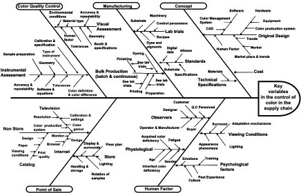
In color communication, a significant array of variables exist that need to be clearly identified, understood and ultimately minimized. A fishbone diagram can be used to depict some of the most important factors in the communication and control of color in the textile supply chain. The sources of variability in the control of color through the supply chain can be broken down into the following broad categories:

Concept;

Manufacturing;

Human Factor;

Color Quality Control and;

Point of Sale

3 Manufacturing

Color Quality Control

Type of instrument Instrumental Assessment Calibration & specification Geometry Sample preparation Software & equations Accuracy & repeatability Key variables in the control of

color in the supply chain Lab trials Machinery Dyes and pigments Recipes Control parameters Substrate Concept Technical Specifications Cost Materials Original Design Hardware Software

Market place & trends Human Factor

Trends Market Color Management

System Equipment Color production system CAD

Point of Sale

Store Floor plan Display & surrounds Handling & storage Rotation of samples Lighting Non Store Television Internet Catalog Calibration & settings Resolution Color gamut Color production system Design Monitor Browser Paper Viewing

conditions Print_quality Design Human Factor Viewing Conditions Adaptation mechanisms Surround Lighting Appearance phenomena Psychological factors

CulturePast Experience Emotions Training Physiological Acquired color deficiency Fatigue Gender Inherited color deficiency Age Standards Digital data Atlases Substrate Specifications Bulk Production

(batch & continuous) Dyeing Finishing Preparation Printing See lab trials See lab trials See lab trials Color definition & color difference Tolerances Visual Assessment Accuracy & repeatability Geometry Booth & specifications Human factor Material type Environmental conditions Tolerances Observers Q.C Personnel

Operator & Manufacturer Customer

Buyer Designer Manufacturing

Color Quality Control

Type of instrument Instrumental Assessment Calibration & specification Geometry Sample preparation Software & equations Accuracy & repeatability Instrumental Assessment Calibration & specification Geometry Sample preparation Software & equations Accuracy & repeatability Key variables in the control of

color in the supply chain Lab trials Machinery Dyes and pigments Recipes Control parameters Substrate Lab trials Machinery Dyes and pigments Recipes Control parameters Substrate Concept Technical Specifications Cost Materials Technical Specifications Cost Materials Original Design Hardware Software

Market place & trends Human Factor

Trends Market Color Management

System Equipment Color production system CAD

Original Design Hardware Software

Market place & trends Human Factor

Trends Market Color Management

System Equipment Color production system CAD

Point of Sale

Store Floor plan Display & surrounds Handling & storage Rotation of samples Lighting Store Floor plan Display & surrounds Handling & storage Rotation of samples Lighting Non Store Television Internet Catalog Calibration & settings Resolution Color gamut Color production system Design Monitor Browser Paper Viewing

conditions Print_quality Design Human Factor Viewing Conditions Adaptation mechanisms Surround Lighting Appearance phenomena Viewing Conditions Adaptation mechanisms Surround Lighting Appearance phenomena Psychological factors

CulturePast Experience Emotions Training

Psychological factors

CulturePast Experience Emotions Training Physiological Acquired color deficiency Fatigue Gender Inherited color deficiency Age Physiological Acquired color deficiency Fatigue Gender Inherited color deficiency Age Standards Digital data Atlases Substrate Specifications Standards Digital data Atlases Substrate Specifications Bulk Production

(batch & continuous) Dyeing Finishing Preparation Printing See lab trials See lab trials See lab trials Bulk Production (batch & continuous)

Dyeing Finishing Preparation Printing See lab trials See lab trials See lab trials Color definition & color difference Tolerances Visual Assessment Accuracy & repeatability Geometry Booth & specifications Human factor Material type Environmental conditions Tolerances Visual Assessment Accuracy & repeatability Geometry Booth & specifications Human factor Material type Environmental conditions Tolerances Observers Q.C Personnel

Operator & Manufacturer Customer

Buyer Designer Observers

Q.C Personnel

Operator & Manufacturer Customer

Buyer Designer

Figure 1. Key variables in the control of color in the supply chain.

4 Arguably, the most important factor within the textile supply chain is the accurate assessment of color differences between two textile materials. Optimization of the correlation between the visual assessment of color and mathematical models that predict color differences is fundamental to any digital system of color management. However, this requires a clear understanding of the scope and limitations of the assessment methodology and optimization of numerical models.

5 The existing models used to predict color differences and color variation are not optimized because they are based on different sets of perceptual data that have been established under various experimental conditions. Currently, the CMC (2:1) color difference formula is the most widely used standardized color difference model in the world, and is incorporated into standards by many international organizations [7]. In 2001, however, the International Commission on Illumination (CIE) recommended the CIEDE2000. A large dataset was used in the development of the CIEDE2000 formula. The dataset combined four separate experimental data. In addition, Luo et al. reported accuracy of prediction for several formulas using the PF/3 measure of performance. A value of 32.6 for the CIEDE2000 formula vs. 37.9 for CMC (1:1) was reported [8].

6 There is limited information regarding variation of individuals in perception of small color differences [9]. Information regarding observer variation may be limited because studies involving perception of small color differences employed a limited number of observers. Most of the studies reported have shown inter-observer variability of about 30% and intra-observer variation of about 50% [9].

In addition, variance can be added with different experimental conditions employed in each study. Studies in perception of small color differences have been carried out using a wide range of experimental conditions that not only vary in term of observers but also in terms of psychophysical methods [9], viewing parameters [12-14] and physical presentation of samples [15].

7

1. Research Proposal

1.1. Objectives

The primary goal of the proposed research is to optimize the experimental methodology for the assessment of small color differences and establish the minimum repeatable variability possible among a statistically significant set of observers under highly controlled viewing and illumination conditions. The specific objectives are:

• To carry out a complete analysis of published literature pertaining to color communication and control;

• To investigate the role of observer size and diversity in determining validity of visual assessments:

o Examine the statistical significance of using expert vs. naïve observers.

• To investigate observer variability in small color difference assessments using the following psychophysical methods:

o Pair Comparison Method.

o Gray Scale Method with particular attention to:

ƒ Type of Scale (standard geometric scale and a new proposed scale).

ƒ Size of Scale.

ƒ Sample Separation.

8

• To replicate the highly controlled method in different parts of the world,

• To evaluate the reliability of the experimental conditions.

• To evaluate the performance of existing models and visual datasets based on the results of the replication study.

• To recommend procedures for visual assessment of colored objects that produce minimum variability among observers, and provide maximum correlation with mathematical models.

9

II. Literature Review

1. Human Color Vision

It is perhaps surprising that there is not a complete explanation of how the human color vision system works. Some aspects of the process are now well-established, while others currently remain as ideas, particularly in the area of how we experience the sensation of color [16]. The visual mechanism involves four main areas: The anatomy of the eye, the relationship between the physics of light and the interaction with the eye, the biological process of transforming photons entering the eye into electrical signals relayed to the brain, and the psychological aspect of how we experience sensations [16]. In order to make significant progress in color-related research, it is necessary to understand what is known about the human vision mechanism.

1.1. The Eye

10 Figure 3.Human eye and its principal parts [17].

1.1.1. The Sclera

The sclera is a strong outer membrane that we perceive as the ‘white’ of the eye. Its shape is maintained by the pressure of the internal eye fluids [17].

1.1.2. The Cornea

11 1.1.3. The Iris

The iris is located behind the cornea. It is a colored sphincter membrane with a circular aperture in the center, and its appearance is what determines a person’s eye color. The function of the iris is to control the amount of light that enters the eye. This control of light is done through the circular opening aperture called pupil [18, 19]. The opening of the pupil is usually determined by the level of illumination. The size of the pupil varies from approximately 1.5 mm when in bright light to approximately 8 mm when in darkness [19].The opening of the pupil can change due to non-visual experiences such as arousal [17, 18].

1.1.4. The Lens

The lens is a malleable transparent component of the eye located behind the iris. Its concave curvature can be changed by zonula muscles in order to focus images on the retina located at the back of the lens, when viewed at different distances [17].

12 This explains why, when people reach the age range of 40-50, the ability to focus near objects often becomes difficult and reading glasses are needed [17, 19]. An important aspect of color vision related to the lens is its transparency across the visible spectrum. The lens tends to transmit less light in the blue end of the spectrum, which produces a measurable yellowish hue. The optical density of yellowness increases with age, which may result in different color experiences [17].

1.1.5. The Humors

The chamber between the lens and the cornea is filled with a clear fluid called aqueous humor. It is a clear liquid that serves as a source of nutrition of the lens and the cornea [18, 19]. The large chamber between the lens and the back of the eye is filled with another transparent fluid called the vitreous humor. This fluid has a higher viscosity than the aqueous humor and occupies almost 60% of the volume of the eye [17, 18].

1.1.6. The Retina

13 Figure 4.Shape of rods and cones [17].

Following the retina there is a layer called the pigmented epithelium. This dark layer inhibits light scattering by absorbing all the light that travels through the retina, i.e., all light that is not absorbed by the photoreceptor cells [18].

1.1.7. The Fovea and Macula

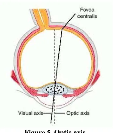
One of the most important sections of the retina is located around the optic axis, where images are focused. The optic axis is an imaginary line that passes through the center of the pupil and intersects the retina in a small area called the fovea [17, 19], as shown in Figure 5.

14 Figure 5. Optic axis.

There are approximately 7million cones and no rods located in the fovea of the human eye. The rods gradually begin to appear when moving away from the fovea [16], which is approximately at an angle subtended to the retina of five degrees. The macula is a larger region of the retina, subtending approximately 20 degrees away from the visual axis, and beyond this region is what may be considered to be peripheral vision [19].

1.2. The Eye and the Brain: How Color Vision Experience is Produced

15 While the precise pathway through the neural cells is not completely understood, it is likely to be a combination of interconnections between the cells. Figure 6 shows a diagram of the cross section of the retina.

Figure 6. Cross-section of the retina [17].

16 Near to the photoreceptors there are the horizontal cells. Other types of connectors are found between ganglion and bipolar cells. They are called amacrine cells [17].

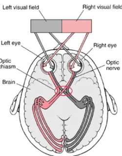
Once the light reaches the photoreceptors a series of chemical transformations occur. The resulting electrical signals are processed by the layers of cells located in the retina (horizontal, bipolar, amacrine, and ganglion). The ganglion cells group together forming the optic nerve [18]. The optic nerve is a neural pathway that exits the eye through an orifice of the retina and the sclera. The electrical data carried through each axon is a combination of the data gathered by the responses from different photoreceptors located in a small region of the retina. The optic nerves from each eye come together to a point called the optic chiasm. At this point the optic nerves cross to the opposite side of the brain and lead to the lateral geniculate nucleus (LGN) which is located in the thalamus, as indicated in Figure 7 [17].

17 The cells in the LGN project the information to the occipital lobe of the cortex in an area called visual area V1. There are near to 30 visual areas in the cortex. The processing that happens inside the different visual areas includes a set of connections that finally allow the humans to have visual perception [18]. Even though it is not well understood, there is evidence that the main visual area related to color perception is V4. It was reported that a woman that suffered a lesion in the right side of the brain close to area V4 was able to see colors with her right eye, but unable with the left eye [17].

1.2.1. Receptive Fields

Receptive field is a term that refers to the concept of how the cells respond to a visual stimulus. The receptive filed is a representation of an area in the visual field for which a cell reacts. The type of response can be positive, negative or spectral bias and it is represented in a specific area of the receptive field. The response of a cell is determined from the input of different photoreceptors. Figure 8 shows a receptive field of a ganglion cell.

18 The Figure illustrates the opposition between center and surround. The positive central response represents the positive input from a single cone surrounded by a negative response input from several cones. This type of response is known as on-center. The negative central response shown in Figure 8b demonstrates response of contradictory charge. This type of response is known as off-center. On-center and off-center responses form part of a dynamic system that allows perceiving the changes in a visual scene [18].

There are several types of ganglion cell responses that may occur during the visual process. However, the concept of receptive fields works similarly for all of them [18]. Also, the concept of receptive fields is used at the LGN. The cells at LGN work similarly to the ganglion cells in the retina. The LGN receptive fields can be thought as representing a massed retinal input since multiple neural fibers from the retina converge to each LGN [20].

1.2.2. Rods and Cones

The photoreceptors convert the light entering the eye into electrical pulses that are processed by the brain. There are approximately 120 million photoreceptors in each retina, although the quantity varies from individual to individual [16]. The quantity and distribution of rods and cones varies with the angle subtended to retina, with zero degree being the visual axis. One of the most important distinctions between rods and cones is their sensitivity to light.

19 The presence of two types of photoreceptors suggests two different visual functions. Around the 1860’s Max Schultze, a retinal anatomist found that animals that function better during nighttime, such as owls, have only rods in the retina. However, Schultze found that animals entirely active during the day, such as pigeons, have only cones, while those animals that are active during both the day and night, such as monkeys, have retinas with rods and cones [17]. These discoveries led to the duplex retina theory of vision. In this theory the rods are used for vision under dim light (low luminance) and the cones are used for bright light. Vision where only the rods are active is called scotopic, whereas vision due to cone responses only is called photopic. Mesotopic vision is when both rods and cones are active.

The photo-active component of both rods and cones is a pigment-protein complex, which absorbs light within a particular wavelength range depending on the nature of the protein. The pigment-protein complex involved in the rods (scotopic vision) is called rhodopsin [21].

20 1.2.3. Monochrome Vision

The process resulting scotopic vision using only the rods can be generally described in three very rapid steps: isomerization via photon absorption, protein conformational change due to isomerization, and the translation of the physical change within the photoreceptor to an electrical signal that is received by the brain. When a photon is in the visible region of the spectrum the free rotation occurs resulting in the formation of all-trans retinal [23].

1.2.4. Color Vision

A similar three-step process for monochrome vision applies to photopic vision, although three cones with differing spectral sensitivity are involved. It is because of the differences in spectral sensitivity of the cone cells that humans with normal color vision are able to distinguish a vast range in colors.

21

1.3. Mechanisms of Color Vision

No unified theory of color vision exists today. However, there are three theories that have been shown to explain certain key aspects of visual perception pertaining to color.

1.3.1. Trichromatic Theory

The existence of three cone photopigments in the retina implies that humans are trichromatic. Thomas Young was the first to suggest that human color vision was thricromatic. However, this fundamental theory was developed more comprehensively by Clerk Maxwell and Hermann von Helmhotlz in the mid 19th century. This theory states that humans perceive color as the result of a mixture of three primary wavelengths corresponding approximately to the sensitivity of red, green and blue regions of the spectrum [18]. The theory has merit as evidenced by the later determination of the three types of cones by George Wald and Paul Brown, in 1959, at Harvard and William Marks, William Dobelle, and Edward MacNichol at Johns Hopkins [25]. In fact, this theory forms the basis of colorimetry today (see section 3 for a discussion of colorimetry).

1.3.2. Hering’s Opponent – Color Theory

22 According to Hering, when mixing yellow and red lights, a yellowish-red perception will result. However, when mixing blue and yellow lights a perception close to white may be experienced. Hering proposed that such colors ‘oppose’ each other. His theory was based on the existence of three opponent color channels located in the retina: red versus green, blue versus yellow and black versus white. These channels respond according to the stimulus wavelength with different polarities [19].

1.3.3. Recent Developments in Color Vision Mechanisms

23

1.4. Mechanisms of Adaptation

The human visual system is sufficiently complex that not only discrete visual processing should be considered, but how the color vision process responds to specific viewing conditions.

1.4.1. Dark Adaptation

24 Figure 9. Dark adaptation recovery [17].

1.4.2. Light Adaptation

Light adaptation refers to the mechanism involved with visual sensitivity when the level of illumination increased, the opposite of dark adaptation, although light adaptation occurs much faster than dark adaptation. The visual mechanism responds to the presence of illumination by decreasing sensitivity in order to identify visual stimuli. This is achieved by shifting from the rod system to the cone system. Light adaptation takes place within 5 minutes. It is comparatively faster than dark adaptation [18].

1.4.3. Chromatic Adaptation

25 One can experience chromatic adaptation when looking at a white object under different types of light, with widely differing spectral power distributions (see Section 3). Although lights differ in terms of wavelength energy, a white object usually appears white despite remarkable changes in incident illumination, providing that the source has emission across the entire visible spectrum. This effect is due to a complex compensatory process that occurs in the cones [18].

1.4.4. Visual Mechanisms Affecting Color Perception

1.4.4.1. Color Memory

This phenomenon is related to the association of an object with an individually perceived ‘ideal’ color. For example, most humans with normal color vision will recall the color of red apples and they are able to reproduce this color without seeing a real object. However, it has been found that the color ‘remembered’ is usually different from the typical real object [18]. Color memory is used in some color matching techniques for the development of; for example, color inconstancy models (see Section 4.2.5).

1.5. Color Vision Deficiencies

26 We can only refer to colors in relation to other colors. However, among the population there are several physiologically-based deviations from the average population that could lead to problems in color perception, some of which are related to color discrimination. Some of these problems can be genetically inherited or acquired.

1.5.1. Inherited Color Vision Deficiency

In relation to the trichromatic theory of color, a number of genetically inherited color deficiencies exist, although their relative abundance in the human population is dependent on geographic location. An extreme example of color vision deficiency is known as achromatopsia in which the cones that do not function, and therefore sight is dependent solely on the rods. People that only use the rod system and have no color discrimination ability and find bright light very uncomfortable. On the other hand, their night vision is normal [17].

A second type of deficiency is when only one type of cone is working in addition to the rods. Individuals who inherit this deficiency are known as monochromats and they have monochromatic vision, resulting in severe problems in color discrimination. However, vision is possible under both photopic and scotopic conditions [17].

27 These individuals are known as dichromats and they have some ability to discriminate color because they still have two types of cones that work. There are three types of dichromats: Protanopes, Deuteranopes and tritanopes. Protanopia is when the individual has an L-cone that is not functioning properly, which results in insensitivity to long wavelengths. A protanope has difficulty perceiving reddish and greenish hues [17, 18]. A well known case of Protanopia is the chemist John Dalton [17], whose published work on color vision deficiencies became known as Daltonism [26].

Deutaronopia is the most common form of dichromacy. A deuteranope is missing the M-cone photopigment; these individuals are still able to respond to green light. However, they have problems discriminating green from some combinations of red and blue [17, 18]. The last type of dichromacy is tritanopia. This type of deficiency is due to the lack or malfunctioning of the S-cone and it is the least common. In this case, the individuals see the long wavelengths as red and the shorter ones as bluish-green [17, 18].

28 Figure 10. (a) Normal vision (b) protanope (c) deuteranope (d) tritanope [17].

The fourth type of color vision deficiency is known as anomalous trichromatism. While individuals with this problem have trichromatic vision, they have a reduced ability to discriminate hues due an alteration in the spectral sensitivities of the photopigments. There are three types of anomalous trichromacy: protanomaly, deuteranomaly, and tritanomaly. The protanomalus has a weak L-cone photopigment or the L-cone absorption is shifted toward shorter wavelengths. The deuteranomalus has a weak M-cone photopigment or the M-cone absorption is shifted toward long wavelengths. The tritanomalus has a weak S-cone photopigment or the S-cone absorption is shifted toward long wavelengths [17, 18]. Table 1 shows the incidence of color vision deficiency in the UK between males and females. Figure 11 shows the incidence of color vision deficiencies in the world [27].

(a)

(b)

(c)

29 Table 1. Incidence of color vision deficiency in the UK[27].

Condition Proportion (%)

Males Females

Protanopia Red-blind 1.0 0.01

Deuteranopia Green-blind 1.0 0.01

Tritanopia Blue- blind very small very small

Protanomaly Red weak 1.0 0.03

Deuteranomaly Green weak 5.0 0.35

Tritanomaly Blue weak very small very small

Figure 11. Percentages of Incidence of defective color vision around de world[27].

1.5.2. Acquired Color Vision Deficiency

30 Table 2 summarizes some of the main differences found between deficiencies acquired and inherited.

Table 2. Summary of common differences between hereditary and acquired color vision deficiencies.

Hereditary defects Acquired defects

Mainly problems discriminating red-green Mainly problems discriminating yellow and _blue

More common in males Common in males and females

Usually present in both eyes Regularly presents a difference in severity between eyes

Problem not associated with color naming It can be associated with color naming _errors Deficiency stable through time Deficiency may present differences through

time

Identifiable with standard color test It requires more than clinical color test to _{identify them} Not related to illness or toxicity Associated with ocular or systematic _{disease or toxicity}

1.5.2.1. Chromatopsia

31 1.5.2.2. Cerebral Achromatopsia

This deficiency can be acquired following a lesion (perhaps following surgery) on the area V4 of the brain, which is the area believed to control color processing [16].

1.6. Color Testing Methods

1.6.1. Ishihara test

32 Figure 12. An example of pseudo-isochromatic Ishihara confusion plates.

1.6.2. Farnsworth –Munsell 100-Hue Test

This test requires observers to order a series of colored chips of constant lightness and chroma but varying hues of just noticeable difference. It was designed to determine the level of hue discrimination among observers, and enables the categorization of observers with normal color vision into different levels of hue discrimination capability, relative to the average population: superior, average and low. Also, the test allows the determination of hue regions of confusion for people that have color deficiency [29].

1.6.3. Neitz Test

33 1.6.4. Cambridge Color Test (CCT)

The Cambridge Color Test was developed with the idea of measuring hue discrimination in a spatial and luminance noise situation [29]. CCT is a computerized test that allows the change of parameters in the stimulus and the threshold detection between pairs of target and background hues [29].

1.6.5. Color Vision Test Made Easy

34

2. Psychophysics

Color is a personal, physiologically-based experience. Researchers have been investigating links between stimulus and the human experience for centuries. At the heart of color science lies the critical issue investigating light interaction with objects and the visual experience. ‘Color’ can be expressed quantitatively as, for example, the amount of light reflected by an object, but the resultant human experience when the visual stimuli is perceived by the eye and brain is not objective, is complex, and varies widely from person to person. Different approaches have been developed in order to understand and ultimately quantify the relationship between experience and stimuli that in some way are defined the composition of matter.

2.1. Definition

Psychophysics has been defined as the “study of the relationship between the physical stimuli in the world and the sensations about them we experience” [31]. Hence, psychophysical techniques allow quantitative determination of a person’s experience to a given stimulus.

2.2. Historical Overview

35 He believed that there was a need for a scientific approach to understand the philosophical issues between mind and body [31]. For this purpose, he proposed three approaches: Detection, Discrimination and Scaling. Detection has as a goal the development of a method to measure the minimum amount of stimuli that can be perceived. Discrimination is the development of a method to determine how much a given stimuli must be varied in order to perceive a difference, and scaling is the development of an approach to quantify a particular dimension of our sensation (e.g. lightness) [31].

Numerous developments have been made since Fechner’s first approaches to understanding perception. Around the 1960’s Stanley Smith Stevens advanced Fechner’s idea of scaling. Stevens studied the relationship between stimulus intensity and perceptual magnitude using a magnitude estimation technique. His findings allowed him to hypothesize that the relationship between stimulus intensity and perceptual magnitude resulted in a power law with various exponents according to perception studied. Stevens’ precepts are important for the perceptual phenomena of color and his statements are found to be elementary in understanding color measurement [18].

36 The various methods developed, summarized below, enable collection of useful perception data, although different approaches will lead to different aspects of perception.

2.3. Detection Techniques

This group of psychophysical techniques is focused in how the sensory systems respond to changes of energy. Energy can be found in different forms of stimulation such as: electromagnetic (light), mechanical (sound, touch, movement), chemical (taste, smells) or thermal (hot, cold). The main idea of detection theory focuses on how much energy change, starting at zero, is needed in order for the change to be perceived by a person [31].

In color perception, these types of techniques are very useful for evaluating tolerances especially in color difference studies. A number of threshold experiments with different levels of complexity in experimental design have been developed with varying levels of significance of data obtained. Some of the most important threshold techniques are: method of constant stimuli, method of limits, and the method of adjustment [18].

2.3.1. Method of Adjustment

37 One of the disadvantages of this technique is that the observer has control over the stimuli and can bias the results due to observer variability. This method is sometimes used in color perception studies as a starting point to design more complex experiments [18].

2.3.2. Method of Limits

This method is more complex than a simple method of adjustment. In this method, the experimenter presents the stimuli at different levels of intensity, the levels of which have been determined prior to executing the experiment. The sequence of stimuli can decrease or increase as necessary. If using an ascending sequence, the researcher starts with a stimulus intensity that is not noticeable and asks the participants to determine and respond if they perceive the stimulus. The stimulus intensity is increased until the stimulus is obviously perceptible. The threshold is calculated by taking the average stimulus intensity in which the transition from not perceptible to perceptible took place. To minimize adaptation effects, it is suggested to do runs of ascending and descending sequences and then average the results [18].

2.3.3. Method of Constant Stimuli

38 The data acquired can be used to produce a psychometric function also known as a frequency of seeing curve. This curve allows determination of the threshold and its ambiguity. Usually a psychometric function can be obtained for an individual person (through multiple repetitions) or for a population of people (one or more repetitions for participant).

The method of constant stimuli can be classified into two methods according to the type of response acquired during the study: The yes-no method and the forced choice method [18]. The yes-no method is extensively used in color science studies where the measurement of visual tolerances is required. For this purpose, an anchor pair with a predetermined color difference is fixed and different pair samples with various color differences are presented to the observer. The observer is asked to determine if the presented stimulus is below the intensity of the anchor pair (pass) or above the anchor pair (fail) [18].

2.4. Matching Techniques

This type of psychophysical technique was developed to determine when two stimuli are not perceptibly different.