Error analysis of the fixed point RLS algorithm

Error Analysis of the Fixed Point

RLS Algorithm

Tulay Adali

Sasan H. Ardalan

Center for Communications

and

Signal Processing

Department of Electrical

and

Computer Engineering

North Carolina State University

ABSTRACT

I. INTRODUCTION

The performance of adaptive algorithms in a finite precision environment is difficult to analyze, but is a very important problem. Because of this complexity of the problem, previous approaches to finding closed form expressions for error had assumed that the input is a white Gaussian random process [12],[1]. In this work, the input is considered to be a. wide sense stationary signal with correla.tion, which is a better model for an actual input signal. The performance criteria used in the analysis is the error vector 8

'(n),

which is defined as the difference between the fixed point weight vector estimate at timen, w'(n), a.nd the optimum system weights, w ". TIle norm square of this value, i.e. the steady state mea.n square prediction error is then derived for the fixed point RLS algorithm, both for the exponentially windowed, and the prewindowed growing memory RLS algorithms.

It has been previously predicted that the convergence rate of the adaptive algorithms depend on the eigenvalue spread of the input autocorrelation matrix, [6],[11]. Particularly for the RLS algorithm, normalized minimum eigenvalue of the input autocorrelation matrix is shown to be the most important factor in determining the convergence rate in [6], by an approximation for the estimator covariance matrix for the prewindowed case. In this work, this result is derived analytically and the importance of other factors on convergence rate is also investigated.

In this work, the problem is stated as a system identification problem. Two calculations are considered to be the most important: the calculation of the weight vector update, and the calculation of the prediction of the desired signal d(

n)

which is through an inner product of the weight vector and the vector of delayed elements of the input samples. The weight vector correction in the update equation is obtained by multiplication of the Kalman gain vector and the scalar prediction error. The quantized version of the Kalman gain is assumed to be available. With this assumption, the results of this paper becomes applicable to the ca.ses where different algorithms are used to compute the Kalman gain.

II. RLS

ALGORITHM

The problem is modeled as a linear system with input signal x(n), and output signal d(n).

The response of the system available for measurement at the filter input

z(n),

is the sum of the desired signal d(n), and a random, additive white noise component, v(n).

z(n)

==

d(n)

+

v(n) (1)

The samples d(n) can then be writ ten in terms of the system impulse response coefficients, w" as

N-l

d(n) = w·Tx(n) =

2:

wix(n - i)

i=O

(2)

where boldface letters denote the vector quant.ities of length N. It is assumed that the system response has insignificant terms beyond N sa.mples. The sample vectors, then have the last N samples of data; that is the input data vector at time n is

x(n)

==

[x(n) x(n - 1) ... x(n - N

+

l)]T . (3)

Now, consider the system identification problem where the system parameters w " are to be estimated. In t he RLS algorithm, the weights w( n) are calculated such that the accumulated sum of the error residuals is minimized. The error residual is the difference between the output of the system, z(n) and an estimate of the desired response obtained from w(n), at time n,

and the quantity minimized is

€(n) == z(n) - xT(n)w(n)

n

€(

n)

==

2:

,n-i€2(n)

i=l

(4)

(5)

where, is the forgetting factor and is chosen less than one. In the RLS algorithm, the current weight vector w( n) is updated through the following recursion,

w(n)

==

w(n - 1)

+

e(n)k(n)

where

e(n)

==

z(n) - xT(n)w(n -

1).

The gain vector, also called the Kalman gain is given by

[14],

(6)

(7)

k(n)

R-1(n)x(n)

III.

FIXED POINT ROUNDOFF ERROR ANALYSIS

To analyze the degradation of the RLS algorithm under fixed point implementation, the same model as in

[1]

is used. The error introduced by rounding the product in the ithentry of (6) is represented by Ili(n), and the roundoff error introduced by the inner product in

(4),

by

f(

n). These roundoff errors are modeled as additive white noise processes with zero mean and variances

[13],

u~

==

2-2B~

/12

and

u;

==

2-2B f

/12 .

B,." and B, are the register lengths in bits, used for the fractional part of the weights and tile data respectively. This model is commonly used for finite register effects

[13],

and is quite accurate if the quantities that are multiplied do not become very small and if the step size, his chosen such that

(f;/

h

is a considerably large quantity [8], which is most often the case. This ratio is a measure of the signal dynamic range and here,

0';

is the variance of the input. Assuming that the Kalman gain, k( n) is precomputed in infinite precision, the ith entry of the quantized gain vector, k~(n) is

(9)

where {3(n) is the quantization error. The same quantity can also be used to model the fixed point errors if k(n) is computed in finite precision.

The error vector

6'(

n) is then defined as the difference between the fixed point weight vector estimate at time n, w'(n), and the optimum system parameters, w ".

6'(n)

==

w'(n) - w*

(10)

It can be then shown that

[1],

the weight error vector can be written as the sum of two vectors

8'{n)

==

x{n)

+

1jJ{n)

where

and

1jJ(n)

=

t,

lift

[I

~

k'(i)XT(i)]] e(i)

together with the definition

nj=n+l[.]

==

1.

Here, e{n) is defined as

e(n)

==

k'{n)1J{n)

+

I-t(n)

where

1J(n)

==

v{n) - €(n).

(II)

(12)

(13)

(14)

If the covariance matrix of the error vector is defined as

Ro,(n)

=

E {8'(n)ll'T(n)}

then, the expected value of the norm of this weight error vector is given by

E

{118'11

2}

=

Trace [Ro,(n)] .

The weight error vector covariance matrix can also be written as

R8,(n)

=

Rx(n)

+

R,p(n).

Here, R x(

n)

and R,p(n) are defined similar to (16).

(16)

(17)

IV.

SUMMARY OF RESULTS

The covariance matrix of two vector components of the weight error vector (11), can be written as:

(19)

and

(20)

where P is the real ortogonal matrix introduced by the congruent transformation

(21)

Since R;.' is real and symmetric, it can be dia.gonalized by this congruent transformation and D;l is a diagonal matrix with 1/Ai'Son the diagonal. Ai'Sare the eigenvalues of the true autocorrelation matrix Rx •

The variables, De(i) and S(k) are defined in equations (53) and (57) In Appendix B, respectively.

A. The prewindowed growing memory algorithm, ,

==

1

For the prewindowed case we have (53) in Appendix B,

(22)

and

(23)

Here, 8(k) ca.n be approximated by an exponential matrix if Q m a z (k)

=

(-/e2

+

/e~~in) is small (60,61). Then, if we break up

R,p(n)

into two and write it as seperate summations as ill (62) with C(M,n) as the partial summation from 1 to At -1 which is also the transient term. In this term, M is chosen such that ama~(k) is considerably small for k ~ 1\.{ and this choice depends on the ratio N

u;/

Amin. A large index 1\1 is needed if this ratio is la.rge. Also, for this chosen M we have limn-+_oo C(1\f,n)

==

o.

Hence, convergence is slow

At the steady state, for n

»

A·!we have

n NU2U 2 u2

R,p(n)

==

u2- I

+

a: #-1R-1

+

~R-l

#-13 2 x n a : .

An expression for R_x can also be derived as

(24)

(25)

where lC is the Euler's constant and is equal to 0.57721. This is the transient term and rapidly dies out. Initial value of the weight error vector, quantization error variance O"~, and most important of all the ratio N

u; /

Amin determine the rate of decay for the terms of this matrix.

At steady state, the expected value of the weight error norm is given by

(26)

when u~

«

1. Except for the highly correlated case, the third term is quite insignificant, leaving the first two in the error equation. The roundoff error variance o~ is typically much smaller tha.n u~, the additive noise component. Hence, correlation enhances this additive noise error initially in the weight error but its effect eventually dies out as the number of iterations increases. The random walk phenomenon due to roundoff errors in the weight update dominates, leading to the divergence of the algorithm. In an earlier work

[10],

it was predicted, indirectly through the sensitivity analysis, that the mean square prediction error is the same for both correlated and uncorrelated signals and this was shown by simulations in [3]. This paper verifies this result by exact analysis. However, this work also considers additive noise and shows that, if the signal is highly correlated, the effect of additive noise also increases and causes divergence.

Both error equa.tions, (26) and (32) reduce to the forms derived in

[1],

if the data is uncorrelated, i.e. all eigenvalues are equal to

u;.

B. The exponentially windowed algorithm, 1

<

1

For this case,

(27)

and

( ( 1 - I )

2 2)

2(

1 - I )

2 -1

( )

S(k)=

1-2 1-')'k+1

+NO"zO"f3

+NO"z

_{1_')'k+ 1} D;". 28

matrix is equa.l to (81):

R,p(n)

=

P ((

CT~I

+

CT~(1

-

l'

)20;1

)0~1)

pT

(29)

D;

=

(2(1-1')-NCT~CT~)I-(1-1')2NCT~0;1

(30)

for (J"~ ~ 1 . The terms of the diagonal matrix Do: are all positive if , is chosen such that

2 N(J"2

_ _ > __

z

1 - , Amin

(31)

is satisfied. Also, the partial summation limn ---.oo

C(M,n)

== O. Actually this is a

non-restrictive requirement since in practice, is chosen such that the memory time constant To == 1/(1 - ,) matches the expected variation of parameters. They should be almost constant over a period of To, which requires To ~ N, [14J.

Using the same definition (20), R_x can again shown to be a rapidly decaying matrix.

Thus for the weight error norm at steady state we have

(32)

This error expression

(32),

indicates that correlation affects the error term associated with the additive noise component which also incorporates the effect of inner product error,

f(

n);

but it does not affect the term associated with the roundoff error due to weight update

recursion.

Correlation A mplification Factor

To account for the impact of correlation on error, we define a new quantity v, the correlation

amplification factor as

(33)

The characteristics of this new quantity, v as a function of signal correlation is analyzed by modeling the input as a first order AR process with AR constant a, i.e.

x(n)

==

ax(n -

1)

+

u(n)

(34)

where u(n) is a white random process. We have in Figure 1 the amplification factor v,

quite typical, since when we let a ~ 1, we are approaching the unit circle, and the input is becoming ill-conditioned.

Tradeoff in Selection of Forgetting Factor 1

V.

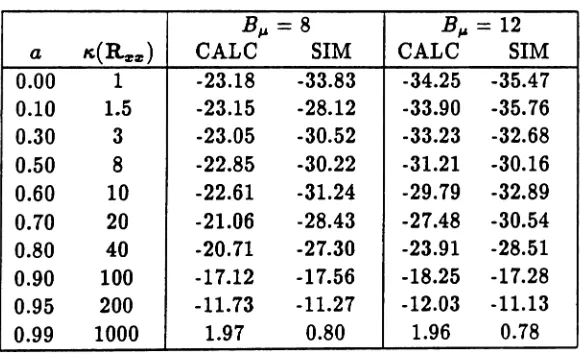
SIMULATION RESULTS

The input used in the simulations is a first order AR (Autoregressive) process, with AR constant a, and the innovation is a white Gaussian random process with unity variance. The input into the system is always normalized such that it has a variance of one. To compa.re the spectral dynamic range of the input, the condition number

K(R:c:r)

is also calculated which is defined as the ratio of the maximum eigenvalue to the minimum in the input autocorrelation matrix, Rx x . The same system identification problem described in section 2 is simulated. The order of the system used in the simulations is 7, and the variance of the additive noise is 0.1. In the simulations, 14 bits are used for the fractional part of the data and 12 bits for the Kalman gain. The approximate values for the condition number are also given in Table 2 for the corresponding pole a, of the AR process.

In Table 1, E

{1I8'(n)I/2}

1Sgiven for various a's, first using t.he error expressions derived in this analysis, equation (32), and then using those calculated by simulation. The number of bits used for the weight vector, Bp, is 9. When the two are compared, it is seen that they a.gree very closely, especially for, == 0.999. But clearly, the predictions a.bout divergence also hold for the second case. In fact a discrepancy between the calculated and simulation val ues is expected as , decreases since, is assumed to be very close to one in the analysis, and this is most often the case in applications. In Table 2, the weight error values are given for two different register lengths, B#J. for, == 0.999. The first term in equation

(32) is dominant especially when correlation is small, which is expected since less bits are being used to represent the data. But it should be also noted that the effect of register length becomes almost ineffective when correlation increases. Since the model used for t.he roundoff errors in the analysis is a better a.pproximation for longer register lengths [13], there is a significant discrepancy between the calculated and theoretical values for B#J. == 8,

especially for smaller values of a, i.e. in the region where the weight roundoff error is more effective.

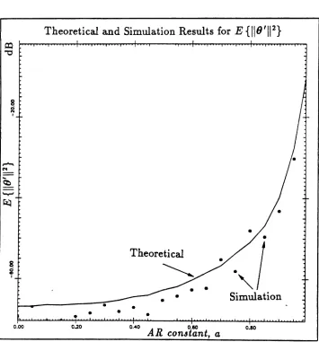
In Figure 2,

E{116'(n)11

2} is plotted as a function of the AR constant a for a system of order 9. The curve is calculated using the error expressions derived in this analysis, equation (32), and then using those calculated by simulation. The forgetting factor is ,

==

0.999 and the number of bits to represent the fractional part of the weights is B#J.

==

10. In Figure 3, the

simulation results for

E{118'(n)11

2

} is plotted as a function of the AR constant,a for different

system orders: 3,5,7, and 9. The same characteristics as in Figure 1 is observed, since the most important term in

(32)

is the amplification factor v. The transient characteristics is shown in Figure 4 for three different AR constant values: 0, 0.6, and 0.9. The ratio N

(J';/

~

is also evaluated for each case, and clearly convergence is slower when the dynamic range of the data is high.

If, instead of the former definition, the weight error norm is defined as the difference between the infinite precision weights and the fixed point weights, such that:

the effect of the additive noise is eliminated, and the roundoff error due to weight update becomes the major error source, [1]. From (1) a.nd (2) it is seen that the term associated with this roundoff error, the first term, does not depend on signal correlation. Although it is not derived here, it is predicted that the error defined in (4), E

{lle'(n)11

2

} does not diverge

VI.

CONCLUSIONS

The steady st ate mean square prediction error is derived for the fixed point RLS (Recursive Least Squares) algorithm, both for the exponentially windowed RLS (forgetting factor,

ApPENDIX A

For l' close to

1,

we have,

[1]

where R(

i)

is defined as

i

R(

i)

==

L

,i-ix(j)xT_(j).

i=O

From (8), we have

(36)

(37)

(38)

Since

R-l(i)

is slowly varying with respect to the product x(i)xT(i) for, close to one, by

the averaging principle

[7],

we have

E{k(i)xT(i)} - E{R-1 ( i ) } E { x ( i ) xT(i)}

(1

~-,~1)

R;lR

z

(1

~~~1)

I.

Similarly, we can derive

Using the definition for the Kalman gain

k(i)

we get

(39)

(40)

Note that the term (xT(i)x(i)) is a scalar term and is equal to the norm of x(i) which is given

by

N-l

Ilx(i)II

2

L

x2(i -

k)

k=O

- Trace [R~]

So, this term is slowly varying with respect to the other terms in the equation. Again, by a.pplying the averaging princi ple [7], we can seperate this expectation from the others. Also, since this is a scalar term, we can change its place in the product, and we end up with

E

{R-1(i)x(

i)xT

(i)x(i)x

T

_{(i)R;1 }}

(43)

Since t3( n) is uncorrelated with the data sequence x(n) we have

For, == 1, we have the following relation at steady state [14]:

E {R-1 (

i)}

=

~

R;1 •

1,

Using

(45),

for, ==

1,

the above relations become:

E

{k(i)xT(i)}

=

~I

1,

E {k(i)kT(i)}

=

~2R;1

1,

E

{k(

i)xT

(i)x(

i)kT

(i)}

=

~~;

R;1 .

1,

(44)

(45)

(46)

(47)

ApPENDIX

B

DERIVATION OF THE ERROR COVARIANCE MATRIX

The covariance matrix

R,p(n)

can be written as,

[1]:

n n n

R,p(n)

=

E(>:?:

II

[I -

k'(k)xT(k)] e(i)eTU)

1=1J=lk=i+1

n-;-l

II

[I -

x(n - m)k,T(n - m)]}

m=O (49)

where we make the definition such that I1;;'~o[']

=

1.

In (49)~ since e(i) occu~sbefore in time than k(n), it is uncorrelated with k(n). Also J.L(i)

and(3(1) are zero mean Independent random variables, uncorrelated with each other. Then using these properties we can get

E {J.L( i)J.LT U)

+

17(

i)17U )k'(i)k,T(j) }

O"~I

+

O"~E{k'(i)k'TU)}. (50)

Prewindowed Growing Memorsj RLS Algorithm

Using equation (47), for I == 1, (50) becomes

for i == j

for i :/: j (51)

where the products with R/3' covariance matrix of bbeta(i), are insignificant compared to the other terms involved and are therefore neglected.

Since R;l is a real symmetric matrix, it can be diagonalized by the following congruent transformation, [15]:

(52)

Here, P is a real and orthogonal matrix and D;l is the diagonal matrix with

1/

Ai'S

on the diagonal. Ai'S are the eigenvalues of the true autocorrelation matrix R:r where

i==1,2, ... ,N.

Using the transformation in (52), (50) can be written as

where

0'2

D_e{i)

==

O"~I + .; D;I.

~

Also, by introducing the following rotations,

x(n)

==

Pxp(n) k'(n)

==

Pk'p(n)

(53)

(54)

(55)

the expected value in (49) can be written in terms of diagonal matrices. We also know that the matrices E{I - x(i)k,T(i)}, and E{I - k'(i)x(i)} are also diagonal (46). Hence, by using the fact that diagonal matrices commute,

(49)

becomes

(56)

where

S(k) E

{(I -

k'p(k)x~(k))(1

-

xp(k)k'~(k))}

pT

(I -

E{k'(k)xT(k)} - E{x(k)k,T(k)}

+

E{k'(k)xT(k)x(k)k,T(k)})

P

pT(I - E{k(k)xT(k)} - E{x(k)kT(k)}

+

E{k(k)xT(k)x(k)kT(k)}

+E{,l3(k)xT(k)x(k),l3T(k)})P. ₍₅₇₎

In the last equality, the model given in (9) is used. Now using the equalities derived in Appendix A for the above expected values and also using the transformation in (52), we have,

... ( ) T (( 2

2 2)

NO";

-1)

.:. k

=

P 1 -

k

+

NU:r U(3 1

+

~R:r p ·

Using the congruent transformation once more, the above equality becomes

~()

( 2

2 2)

N

u;

-1 .:. k

=

1 -

k

+

u:r u{3N 1

+

~D:r ·

The exponential function of a matrix is given by [15]:

A A2 e ==I+A+-+··.

2!

(58)

(59)

(60)

which can be approximated by the first two terms if the spectral radius of matrix A 1 is

small. Now, if we let

(61)

A becomes a diagonal matrix and hence its eigenvalues will be its diagonal entries. The maximum eigenvalue of matrix, i.e. the spectral radius of A is determined by the terrn

(k) -

(-2

+

NCT:).

2 ·

11

Orna.:r - T k2~Tnin' SInce U{3 IS a very sma term.

If

orna.:z:(k) is small we can use the first two terms in

(60)

for the exponential approximation.

At this point it is convenient to break upR,p(

n)

into two, and write as seperate summations:

(62)

Here, C(At, n) is t.he partial summation from 1 to Al - 1. This is the transient term, and

},,1 is chosen such that Qrna.:r(k) is a small quantity for k ~ AI. Choice of AI depends on the ratio N

u;/

Amin' a large index 1\1 is needed if this ratio is large. Also, for this chosen

Al we have limn-+CXJC( AI,n) --4

o.

If we consider only the steady state part, we have

R",(n)

=

p ..

t

D

_e(

i)

(n

(e=l

eNIT;'IT~

e;;lD;l))

pT

t=M k=t+l

p

:t

De(i)

(i

2

2

et-i-

eNIT;'IT~(n-i) eNIT~D;l(a.h-nh))

pT. (63)

i=ft.f n

For the summations in the above equation, the following sum formulae are used

[16]:

n

1

~2

1

1/2

(.; k2 =

"6 -

n

+

1 - (n

+

l)(n

+

2)

(64)

(65)

n I l

L

"'7 ~ Ie

+

Inn

+

-2 ·

i=l t n

In (65), 'Yc is defined as Euler's constant and is equal to 0.57721. Neglecting,terms pro-portional to 1/n2 _{and those of higher order and using the well known summations:}

and for n

«

1

(66)

(67)

equation (63) reduces to

for {T~

«

1, and i, n large.

Thus, for n

»

AI we can write

2

2n (T11 1

R,p(n)

=

0""31

+

~R~ ·

where we have neglected all insignificant terms.

(69)

The expression for R_x can be easily derived using the same transformations (52,55) to-gether with equation

(59),

and the summation approximations

(66,65).

Rx(n)

=

0(0)

(g

S(i)) OT(O)

O(O)P

(g

e

-.2

eNu;,u~eNu;,D;;l Z=~=1

-b )

pTOT(o)

(

I N 2 2 N 2D-1 ( 11'2 1)) T

O(O)P

n_{2 e}-2/, ce u rcu13ne Urc "

T-m

(O(O)P).

(70)

The term in the paranthesis in (70) is a rapidly decaying term and Rx(n) does not have a.ny effect in steady state.

Eeponeniiallu lVindowed RLS Algorithm

Using the same transformations in

(52)

arid

(55)

we can reduce the matrix Rt/J(n) to the same form in

(56).

For this case,

and

( )

2

. 2 1 - , 2 - 1

D_e(

1,)

==

{Till

+

.

(TnD:r.

r- 1 _ ,t+1 .,

(71)

S(k)

=

(1 - 2(1

~~:+l)

+

NO";O"~)

+

NO";

(1

~~:+1)

2

D~l.

(72)

For the case where, is close to one and the dynamic range of the input is not very large, we can again make use of the exponential approximation in (60). Then

Rt/J(n)

can be written as

~ n-1,

~ n-i

n n

(_2(---!..=.L.)

22 NCT2(---!..=.L.)2n_1)

R,p(n)

=

P ~

De(i)

Ie!!l

e 1-"J"+t eNurcul3e rc l-"JIi·n: " .

At this point we use the following approximations for the summations:

n 1

IeEl

1 - 1'1e+1

n

1

~

(1 - 1'10+1 )2 k=t+1

(73)

which are quite accurate especially for -y close to one and for large i and n, [1].

Thus, for a sufficiently large index i

=

M for which -yi

«

1, (73) can be written as

Here, Do is defined as

and C(1\,f,n) is the summation

(

~f - I )

C(.M,n)

=

P

t;

De(i)e-(n-i)Da pT.

(76)

(77)

Term of the diagonal matrix Do at jth position, where j is the row or column index, is 2( 1 - ,) - No-;o-~

-

N 0-;(1 -

,)2; ,

where j

==

1,···,N. Terms of this mattrix are all

1

positive if we have

2

(1 - ,) (78)

where we have neglected the term N(j;(j~ which is a very small number with respect to the other terms involved. Hence, for la.rge n, and when (78) is satisfied, we have limn_ooC(Af,n) ~

o.

Also, since the approximations used in the summations

(74)

are better approximations for large indices they give better results in steady state. Here, C(1\11,n) is the term associated with the transient period and rapidly goes to zero if (78) is satisfied. Actually, this bound is discussed in Section VI, and it is shown that this condition is easily satisfied with the choice of " in practice.

Using the summation formula for matrices:

n

LA

i

₌₌

_{(I -}

_An₊1

_{)(1 -}

_A)-I.

i=O

we can write

n

L

eDa(i-n)

=

e-nDa(eMDa - e(n+l)Da)(I_ eDat l.

i=M

(79)

Since D_a has positive entries, d_{a i} ~ 1, for (n ~ M) we have (-n

+

J\,f)Da --+

o.

Then, we can write

n

L

eDa(i-n) ~ [eDa(eDa - I t l].

i=M

Using this summation formula (80), we can rewrite (75) as

(81)

Now let us reconsider equation (76). If

"min,

the minimum eigenvalue of the autocorrelation matrix is not very small, or if l' is chosen very close to one when Amin is very small, the

first term in matrix Da , (76) will be dominant and the covariance matrix will be

(82)

References

[1] S.H.Ar?alan, ?-nd S.T.Alexander, "Fixed point roundoff error analysis of the ex-ponentially windowed RLS algorithm for time varying systems" IEEE Trans. Acoust.,Speech,Signal Processing, vol. ASSP-35,No. 6, pp. 770-783, June 1987.

[2] E.Eleftheriou, and D.D.Falconer, "Tracking properties and steady-state performance of RLS adaptive filter algorithms," IEEE Trans, Acou3t.,Speech,SignalProcessinq, vol. ASSP-34,No. 5, pp. 1097-1109, Oct. 1986.

[3]

S.II.Ardalan, and T.AdaII, "Sensitivity a.nalysis of transversal RJ.JS algorithms with correlated inputs," in Proc. ISCAS 89, May 8-11 1989, Portland, Oregon, vol. 3, pp. 1744-1747.

[4] T.Adah , and S.H.Ardalan, "Convergence and error analysis of the fixed point RLS algorithms with correlated inputs," in Proc. ICASSP 90, April 9-6 1990, Albuquerque,

New Mexico,

[5]

T.Ada.ll, and S.H.Ardalan, "Stea,dy state and convergence characteristics of the fixed point RLS algorithm ,'1' in Proc. ISCAS 90, lv/ay 1-3 1990, New Orleans, Louisiarui.

[6] J.M.Cioffi, and T.Kailath, "Fast, recursive-least squares transversal filt.ers for adap-tive filtering," IEEE Trans. Acoust.,Speech,SignalProcessinq, vol. ASSP-31,No. 6, pp. 1177-1191, Oct. 1983.

[7] C.Sa.mson, and V.U.Reddy, "Fixed point error analysis of the normalized ladder algo-rithm," IEEE Trans, Acou.st.,Speech,Signal Processinq, vol. ASSP-31,No. 6, pp. 1177-1191, Oct. 1983.

[8] C.W.Ba.rnes, B.N.Tran, and S.II.Leung, "On the statistics of fixed point roundoff er-ror," IEEE Trans. Acoust.,Speech,Signal Processinq, vol. ASSP-33, pp. 595-606, June. 1985.

[9] 11.Bellanger, and C.Cengiz, "Coefficient wordlength limitation in FLS adaptive fil-ters," Proc. ICASSP 68, Apr. 7 1986, Tokyo, Japan, pp. 3011-3014.

[10] S.H.Ardalan, "On the sensitivity of RLS algorithms to pert.urbations in the filter coefficients," IEEE Trans. Acou.st.,Speech,Signal Processinq, vol. ASSP-36,No. 11, pp. 1781-1783, Nov. 1988.

[11] G.Ungerboeck, "Theory on the speed of convergence in adaptive equilizers for digital communication,"

teu

J. Re3 Develop., pp.546-555, Nov. 1972.

[12] S.II.Ardalan, "Floating point roundoff error analysis of the RLS and LMS algorithms,"

IEEE

Trans.

Circuits Sy3t., vol. CAS-33,No. 12, pp. 1192-1208, Dec. 1986.

[13] C.Caraiscos, and B.Liu, "A roundoff error analysis of the LMS adaptive algorit.hm,"

IEEE Trans. Acoust.,Speech,Signal Processing, vol. ASSP-32,No.

XX,

pp. 34-41, Feb. 1984.

[15] S.H .Friedberg,A.J .Insel,L.E.Spence, Linear Algebra, Eagglewood Cliffs,N.J .:Prentice Hall,1989

i

=

.999 i = .99

a

CALC

81M

CALC

81M

0.00 -31.96 -35.96 -24.43 -31.31 0.10 -31.89 -32.97 -24.30 -27.98 0.26 -31.47 -32.33 -23.60 -26.31 0.50 -29.85 -30.13 -21.19 -23.89 0.60 -28.58 -30.27 -19.54 -21.38 0.70 -26.66 -28.31 -17.26 -19.45 0.80 -23.62 -22.81 -13.90 -15.27 0.90 -17.93 -18.26 -8.01 -12.96

0.99 1.92 0.48 11.90 6.41

Table 1: Weight Error for B#Jt

=

9, in dBs

B#Jt

=

8 B",

=

12

a It(~z)

CALC

81M

CALC

81M

0.00 1 -23.18 -33.83 -34.25 -35.47 0.10 1.5 -23.15 -28.12 -33.90 -35.76 0.30 3 -23.05 -30.52 -33.23 -32.68 0.50 8 -22.85 -30.22 -31.21 -30.16 0.60 10 -22.61 -31.24 -29.79 -32.89 0.70 20 -21.06 -28.43 -27.48 -30.54 0.80 40 -20.71 -27.30 -23.91 -28.51 0.90 100 -17.12 -17.56 -18.25 -17.28 0.95 200 -11.73 -11.27 -12.03 -11.13

0.99 1000 1.97 0.80 1.96 0.78

5 .~ ~ Q 4 ~ ~ ~ ~ Q ₃

...

~ ~ ~ ~ -... ~ ₂

e

~

0.2 0.4 0.6 0.8

AR constant, a

Figure 1: Amplification Factor, v

Theoretical and Simulation Results for E

{1I

8'112 } 8_o N,

•

8 g I 0.00 0.20

•

•

Theoretical

•

•

•

0 .• 0 A 0.60

R constant, a

."

Simulation

0.80

o

N o

8

o

Mean Square Prediction Error

- _ _ N=9

--- N = 7 -_···-.·N=5 _._._-- N

=

3

0.00

I

Q.20 0.40 0.80

constant, a 0.80

Mean Square Prediction Error

o

N

0';/

Amin

=

9.83 for a = 0.0

0 ₌ 55.96 for a

=

0.6

N

I

=

880.03 for a

=

0.9

e

.

I

~

C"'lI

-(z)

-

0-0.1

~I ~t

i

I

o 100

200 iteration» 300 400