An Empirical Study of the Tacit Knowledge Management Potential of Pair Programming

(1)

ABSTRACT

Wilson, Dylan Garrett. An Empirical Study of the Tacit Knowledge Management Potential of Pair

Programming. (Under the direction of Laurie Ann Williams.)

This work describes an experiment comparing knowledge sharing in two distinct team structures.

Given the increasing importance of knowledge in the workplace, especially software engineering, we

are interested in paradigms that can assist in knowledge management. To this end, we conducted an

experiment to determine how the paired or solo programming model affects knowledge sharing

during a software project. We show a pattern of results that suggest pair programming has a positive

effect on knowledge sharing. We also find development time is somewhat higher when using paired

programming, but product quality is unaffected by programming method though these results are not

(2)

An

Empirical Study of the Tacit Knowledge Management

Potential of Pair Programming

by

Dylan Garrett Wilson

A thesis submitted to the Graduate Faculty of

North Carolina State University

in partial fulfillment of the

requirements for the Degree of

Master of Science

COMPUTER SCIENCE

Raleigh

2004

APPROVED BY:

_ _

__________________________

Chair of Advisory Committee

(3)

Biography

Dylan G. Wilson received a Bachelor of Science degree in computer science from Winthrop

University in 2000. After graduating, he entered the graduate program at North Carolina State

University in computer science. In 2000, he also began working for BD Technologies as a software

engineer. In this role he develops bioinformatics tools that supports a team of biologists performing

complex, high-throughput biological experiments. He continues to work at BD today and will

consider pursuing a Ph.D. in computer science in the future. He is especially thankful for the support

(4)

LIST OF TABLES

...V

LIST OF FIGURES

... VI

1. INTRODUCTION ...1

2. BACKGROUND AND RELATED WORK ...2

2.1 P

AIR

P

ROGRAMMING

...2

2.2 K

NOWLEDGE

M

ANAGEMENT

...4

2.3 K

NOWLEDGE

M

ANAGEMENT AND

P

AIR

P

ROGRAMMING

...8

3. EXPERIMENT...9

3.1. E

XPERIMENTAL

D

ETAILS

...9

3.2. E

XPERIMENT

L

IMITATIONS

...13

4. QUANTITATIVE RESULTS AND ANALYSIS...14

4.1 K

NOWLEDGE

S

HARING

...17

4.1.1. G

RAPH

...17

4.1.2 S

CHEMA

...19

4.1.3 E

XTEND

...21

4.1.4 T

ECHNOLOGY

U

SE

...21

4.1.5 C

OMPOSITE

Q

UIZ

S

CORE

...22

4.1.6 M

ETHODS OF

L

EARNING

...24

4.2: I

MPLEMENTATION

T

IME

...26

4.3: I

MPLEMENTATION

Q

UALITY

...27

(5)

5. SUMMARY AND FUTURE WORK...31

6. APPENDICES

...37

6.1. T

EAM

P

ROJECT

P

REFERENCE

F

ORM

...38

(6)

List Of Tables

T

ABLE

1: S

ELF

-A

SSESSMENT

S

AMPLE

C

ALCULATION

...11

T

ABLE

2: S

UMMARY OF PROJECT SIZE METRICS

...12

T

ABLE

3: P

OST

-P

ROJECT

Q

UIZ

O

VERVIEW

...14

T

ABLE

4: I

10: D

ESCRIPTIVE STATISTICS FOR TECHNOLOGY USE...22

T

ABLE

11: S

AMPLE CALCULATION OF COMPOSITE SCORE

...22

T

ABLE

12: D

C

OMPOSITE

...23

TABLE 13: LEARNED ON OWN CONTINGENCY TABLE...25

T

ABLE

14: L

EARNED FROM

T

EAM

C

...28

TABLE 18: QUANTITATIVE RESULTS SUMMARY

...29

(7)

IGURE

5: B

OX PLOT FOR

I

MPLEMENTATION

T

IME

...27

(8)

Knowledge is experience. Everything else is just information. -- Albert Einstein

1. Introduction

As knowledge becomes more important in the economy, those firms that leverage knowledge

efficiently will be more successful [1]. The study of Knowledge Management (KM) has emerged in

response to the heightened importance of knowledge and the need to maximize its usefulness. Much

of early KM research was Information Technology (IT) focused, often concerned with building

software systems to explicitly record, organize, and disseminate knowledge within an enterprise. The

scope of KM research has since broadened and become more multidisciplinary. Specifically, KM

researchers are building a more holistic view of the KM problem, including the social and tacit

aspects of knowledge. The challenge for future KM strategies is to address these social and tacit

aspects of knowledge [2-4].

Our research explores how different styles of work might affect knowledge sharing in small

software development teams. In particular, we compare knowledge sharing amongst advanced

undergraduate student teams of pair programmers versus teams of solo programmers. Pair

programming (PP) [5] is a practice whereby two programmers work together at one computer,

collaborating on the same algorithm, code, or test. Further, the term pair rotation [5] is used to

denote when programmers pair with different team members for varying times throughout a project.

In this thesis, we report the results of a six-week experiment in an advanced undergraduate course

at North Carolina State University (NCSU). The students were tasked with developing a web-based

application in which anonymous course feedback is provided to instructors as a course progresses.

The experiment was designed as an investigation of pair programming with pair rotation as means for

managing knowledge. The students were formed into groups of 4-5 students that were designated as

pair programming groups or solo groups. The solo groups divided the work items, completed the

work alone, and integrated their results. The pair programming groups completed a significant

amount of their task with two team members at one computer, dynamically changing the makeup of

(9)

We hypothesize that when compared with traditional solo group development, software

developed by groups using pair programming with pair rotation will be characterized by the

following:

1. Higher levels of tacit and explicit knowledge sharing as measured by a post-project

assessment/examination of each individual’s knowledge of their overall project.

2. Comparable or shorter development time, implying that knowledge sharing occurred

essentially without cost.

3. Higher product quality, as measured by a set of functional, black box test cases.

In subsequent sections of this paper, we provide background on the experiment and give detailed

analysis of the results. Section 2 gives an overview of pair programming and knowledge sharing.

Section 3 describes in detail the experiment carried out at NCSU. Section 4 presents the analysis of

our results. Section 5 outlines the conclusions and future work.

2. Background and Related Work

A brief introduction to pair programming research results and knowledge sharing follows.

2.1 Pair Programming

Though pair programming (PP) has been practiced sporadically for decades [5], experimental

research into PP is somewhat limited. As early as 1975, Jensen found large improvements in

programmer productivity using pair programming on a 30 thousand lines of code (KLOC) Fortran

project [6]. Nosek ran an experiment [7] in which 15 full-time programmers were organized into

five solo programmers and five groups of pair programmers to write a script that performed a

database consistency check. Both solo and pair programmers were given 45 minutes to complete the

task. Nosek measured the impact of PP on five independent variables: time, readability,

functionality, programmer confidence, and enjoyment. Scores were better for pairs in all measures,

but the differences in the time and readability scores were not statistically significant. The combined

(10)

but does not elaborate, that the scripts produced by some of the pairs were significantly better than the

scripts they bought from expert consultants.

Williams conducted a semester-long experiment using 41 junior/senior-level computer science

undergraduates at the University of Utah in 1999 [8]. Students completed four assignments during

the experiment; two-thirds of the class (28 students) worked in pairs, and the rest of the students (13

students) worked alone. Williams [8-11]observed that at the end of the project, code written by pairs

passed 90% of the acceptance tests while code written by soloists passed only 75%, suggesting a

pair-to-soloist defect ratio of 0.6. The results were statistically significant at an alpha level of less than

0.01. The pairs took 15% more person-hours to complete the assignments than solo programmers.

However, this time increase was not statistically significant. Detailed economic analysis

demonstrated an economic advantage of pair programming over solo programming due to higher

quality and minimal time increase [12, 13]. Williams has also reported anecdotal evidence from

professional software engineers suggesting pairs in industry do not demonstrate this time increase [5].

Nawrocki et al. engaged 21 senior-level students on four different programming projects ranging

in size from 150 to 400 LOC [14]. They divided the students into three groups:

• Extreme Programming (XP) [15] with pair programming (XP-PP),

• XP with solo programming (XP-solo), and

• The Personal Software Process (PSP) [16] with solo programming [16].

The researchers found errors were slightly lower with XP-PP than either of the solo processes. They

also concluded that XP-PP was less efficient than suggested by Nosek [7] and Williams [8], and that

PSP was less efficient than XP-solo. However, the programs were small enough that the research

subjects may not have passed though the inevitable pair-jelling phase [5] in which conditioned solo

programmers learn to leverage the power of pair programming. The four programs implemented in

this experiment were approximately four times longer than in Nosek’s study [7], but were still

(11)

2.2 Knowledge Management

A complete understanding of KM includes the context in which it has emerged and become

important. This context is the shift in the world economy from tangible assets, capitol, and labor to

information and knowledge. One of the early heralds of this new information-oriented economy was

Thomas Stewart in his 1991 Fortune article entitled “Brainpower.” In this article, he pointed to

knowledge as an important but undervalued and under-utilized asset to business [17]. In his later

book, he argues that the economy is undergoing a revolution: “Growing up […] is a new Information

Age economy, whose fundamental sources of wealth are knowledge and communication rather than

natural resources and physical labor.” [1] As pointed out in the original 1991 article, with the

increasing importance of knowledge comes an increasing need to manage it efficiently and

effectively. The field of KM is a formal response to this need.

There is no universally accepted definition of knowledge. Therefore, we summarize various

views of knowledge and create a definition for the purpose of this work. Davenport and Prusak

define knowledge as “… a fluid mix of framed experience, values, contextual information, and expert

insight that provides a framework for evaluating and incorporating new experiences and information.

It originates and is applied in the mind of knowers.” [18]. McDermott emphasizes the social,

especially human, aspects of knowledge saying “knowing is a human act” and that “knowledge is the

residue of thinking” [19]. Horvath defines knowledge in two distinct ways. From a business view he

suggests knowledge is “ . . . information with significant human value added” [20]. From a

philosophical viewpoint, and in agreement with McDermott, he says knowledge is socially

constructed and can therefore, never be cleanly separated from the social interactions under which it

was created. For this reason, KM “should focus primarily on increasing the frequency and quality of

[social] interactions.” [20] Finally, he points out that the differences between knowledge and

information are context dependent. Knowledge in one context may be information in another.

For the purposes of this work, we synthesize these views into a working definition of knowledge.

(12)

creator(s) and the context under which it was created. Knowledge sharing therefore requires a

sharing of both the knowledge and significant portions of the context under which it exists.

Knowledge exists in two primary forms, tacit and explicit. Explicit knowledge is easily recorded,

and exists primarily in a recorded state and requires little or no context beyond what is actually

recorded. Explicit knowledge is not very different from information. Examples of explicit

knowledge are business documents and formal business processes. Explicit knowledge is easier to

manage as its very nature allows it to be separated and stored apart from its creator.

At the far end of the knowledge-information spectrum is tacit knowledge. Tacit knowledge is

very difficult to record and requires significant effort to be converted to explicit knowledge.

Examples of tacit knowledge might include the process of choosing a design pattern to solve a

complex problem or instructions on how to approach the design of a large software system. Tacit

knowledge is built from experience and, as we will explore below, is not easily communicated. It is

not amenable to the same management techniques as explicit knowledge [20, 21].

Horvath describes tacit knowledge as opaque, sticky, time-sensitive, and context-dependent [20].

It is opaque because it is difficult to know what you know and sticky because that knowledge is

resistant to transfer to others. It is time-sensitive because the valuable knowledge, particularly in a

business environment, is constantly changing, requiring continuous refresh and relearning. It is

context-dependent because understanding the knowledge requires an ability to understand the context

under which the knowledge was created and is applicable.

Tacit knowledge is more difficult to manage, but is more valuable than explicit knowledge [20].

For instance, Nonaka claims that the conversion of tacit knowledge to explicit knowledge is where

knowledge creation occurs [22]. Horvath’s central premise is that tacit knowledge is more valuable

than explicit knowledge in four specific areas: innovation, best practices, imitation, and core

competencies [20]. He suggests that innovation is tightly linked to tacit knowledge because tacit

knowledge is quickly developed and used during innovation, before it can be formalized and

(13)

relates this to the insurance claims processors studied by Wenger, suggesting that the processors

worked together to build a tacit set of best practices to get their job done. Imitation is cited because it

is difficult to copy a successful business if the success of the business is due in large part to the

successful management of tacit knowledge. Unless a competitor steals the people that hold the

knowledge, they will not be able to imitate. With respect to core competencies, Horvath says “By

getting a handle on its tacit knowledge assets, a firm can better understand its competitive position

and can more effectively select and shape the markets in which in competes.” [20] Finally, Lindvall

highlights the importance of tacit knowledge in software engineering in particular: “Software

development is a human and knowledge intensive activity and most of the knowledge is tacit and will

never become explicit. It will remain tacit because there is no time to make it explicit.” [23] This

sentiment is echoed by Chou, Maurer, and Melnik: “ … most of the knowledge in software

engineering is tacit.” [24]

Early work in Knowledge Management focused on explicit knowledge and was IT-centric,

attempting to extend techniques from Information Management [21, 25]. McDermott claims that IT

inspired KM but cannot alone bring the KM “vision” to fruition: “The great trap in knowledge

management is using information management tools and concepts to design knowledge management

systems.” [21] Horvath also supports this view by stating that early KM was used primarily to make

explicit knowledge more accessible [20]. Others, such as Nonaka, Wenger, and Baker reinforce the

idea, directly or indirectly, that the application of technology alone is not sufficient to successfully

manage knowledge [22, 25, 26].

Since IT alone will not solve the KM problem, additional techniques have been sought. Given

the definition of knowledge above, the social and human aspects must be addressed if knowledge is to

be managed. McDermott captures the idea: “Leveraging knowledge involves a unique combination

of human and information systems.” [21] One technique that may help with the human aspect of

managing knowledge, particularly tacit knowledge, is the Community of Practice (CoP) [27]. A CoP

(14)

individuals gather, either formally or informally, and share stories and insights gained through

experience. The CoP emerges because individuals cannot know everything and need the community

to succeed in a complex world. According to Wenger, CoP are “organic,” “spontaneous,” and

“informal,” meaning that a CoP naturally forms in a grassroots or bottom-up fashion, often by

necessity and without a formal structure [27]. Lave and Wenger have formalized the CoP and have

highlighted their importance in a knowledge-intensive environment. CoP are a “… privileged locus

for the acquisition of knowledge” and a “privileged locus for the creation of knowledge.” [26]

Unfortunately, the very nature of the CoP puts it at odds with conventional KM. The explicit

management of an emergent, organic, spontaneous, and informal process is not straightforward.

Firms can encourage CoP creation and provide for their existence, but managing and measuring their

contribution to the business has been done only on a very limited basis [27, 28]. CoPs are useful for

transferring and creating knowledge efficiently, but they are difficult to manage. We propose that

there exists a class of hybrid approaches whereby the benefits of the CoP are maintained while the

difficulties associated with managing and measuring their contribution is lessened. We further

suggest that teams of pair programmers are an instance of this proposed CoP-hybrid approach

because they provide a CoP-like environment while retaining a level of manageability and

accountability not present in the CoP. Wenger is clear that team and CoP are not equivalent: “A

community of practice is not just an aggregate of people defined by some characteristic. The term is

not a synonym for group, team, or network.” [26] While CoPs are not teams, a team is not prohibited

from being or functioning similar to a CoP [29]. We leave this as an open question, but point to the

results of our experiment as a positive indication that pair programming teams may be CoP-like.

Our research builds from Palmieri’s work studying KM and PP [30]. Palmieri attempted to

answer three hypotheses related to: (1) whether PP reduced the impact of employee turnover; (2)

whether PP reduced the tendency people have to hoard knowledge, and (3) whether PP has a positive

influence on KM by driving knowledge dissemination and retention. Using a 29-question survey,

(15)

hoarding knowledge but did support the impact reduction of employee turnover, although without

statistical significance. He found, with statistical significance, that “[p]air programming is an

effective means of knowledge dissemination and knowledge retention that has a positive influence on

the Knowledge Management practices of a company or organization” [30]. These findings indicate

PP may be a useful tool for KM. We attempted to confirm these findings by measuring how PP

impacts knowledge sharing when compared to solo programming.

2.3 Knowledge Management and Pair Programming

Recently comparisons between knowledge management in traditional versus agile programming

methodologies has appeared in the literature. Specifically, Chau, Maurer, and Melnik compare and

contrast the differences between agile, such as XP, and traditional programming methods with respect

to KM [24]. The overarching difference presented between traditional and agile methods relates back

to the notions of tacit and explicit knowledge. In traditional programming methods, knowledge

sharing occurs via explicit mechanisms such as documentation. This requires the tacit knowledge of

developers to be converted to explicit knowledge, which can be a time-consuming and high-effort

endeavour, both initially and ongoing. Chau et al. [24] contrast the two methods on several points.

Of particular interest here are the comparisons of agile to traditional methods with respect to

documentation, requirements and training.

Furthermore, agile methods stress frequent and close customer involvement when gathering and

updating software requirements. Traditional methods, on the other hand, are generally oriented

toward exposing and documenting requirements at the beginning, often by a single individual or

individuals who may not actually develop the system. Frequent and close contact allows agile

developers to update and refine their internal model of the problem while the customer updates their

needs. This contact and the communication is largely tacit in nature [24].

Finally, Chou et al. [24] highlight the differences in training between the two methods. In

traditional methodologies, training is highly formalized, easily repeatable, and expensive (takes

(16)

training consists of a junior developer pairing with a senior developer. This can create problems

though, as pair rotation can lead to conflicting information, and may lead to reduced productivity of

the senior developer(s). The researchers suggest a hybrid approach to training based on the strengths

of both methods: “It should be possible to put in place a training infrastructure that has the benefits of

both approaches.”

A recent case study offers anecdotal evidence that XP may provide KM benefits. In the study,

Benedicenti [31] describes how XP played a crucial role in mediating the knowledge-related

problems created by a high-turnover environment. In this study, XP proved to be a very successful

method for transferring knowledge rapidly and efficiently. Further, the use of agile-like methods was

adopted throughout the organization, from junior development staff through upper management.

“Everyone is immediately productive, signifying that the group was effective in transferring

knowledge. This knowledge is not only theoretical … but it is also practical, leading to very fast

development times.” [31]

3. Experiment

In this section, we describe the details of our knowledge sharing experiment and discuss

some if its limitations.

3.1. Experimental Details

We ran a formal empirical study to compare knowledge sharing between PP and solo

programming. The experiment was conducted at North Carolina State University (NCSU) in the

advanced-undergraduate (junior/senior) software engineering course in the Fall 2002 semester. The

140 students attended two 50-minute lectures weekly. Additionally, they attended one weekly

two-hour hands-on lab each week. There were six lab sections of at most 24 students taught by four

teaching assistants. The course had five two-week programming assignments in which the students

(17)

two-week programming assignments and assimilated to the practice of pair programming during these ten

weeks. The experiment was run during the six-week team project.

We divided the students into 34 groups of four or five students, each in the same laboratory

section. The groups were subdivided into three types of development: solo (SO), co-located pair

(CP), and distributed pair (DP). The solo groups were to work “traditionally” in that the work would

be subdivided, assigned to each team member, and later integrated. The co-located paired groups

were to subdivide the work, assign the items to dynamic pairs (practicing pair rotation), and later

integrate paired work. The distributed pair also subdivided the work and assigned work items to

pairs, but unlike co-located pairs, a distributed pair did not work in the same physical location.

Instead, they used collaborative screen-sharing technologies, such as Microsoft NetMeeting™ to

work in pairs over the Internet. Distributed pair programming has been found to be a viable

alternative for academic team projects [32-34].

We used a pre-grouping, self-assessment survey to determine appropriate team composition. This

survey can be found in Appendix A. Since our sample size consisted of only 34 groups, we were

concerned with the potential of any of the three development-type groups being preferred by higher-

or lower-performing students. Therefore, with a focus on forming teams of approximate academic

equivalence, we developed an algorithm for forming teams. The team-forming algorithm was

performed under the following constraints:

• The students were queried to name class members with whom they did not want to

work, and we made a reasonable attempt to respect these requests.

• We avoided any groupings in which there would be only one female in a group.

• We asked the students their preference/ranking of each programming style (SO, CP, or

DP) and considered their preferences. Because the majority of development time

occurs outside of class, the actual use of the programming style could not be

(18)

conformance was to assign students to their preferred programming style when

possible based upon the overall team-forming algorithm.

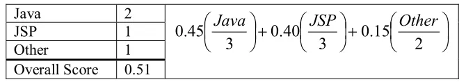
We calculated each developer’s Relative Academic Standing (RAS) as a combination of their

self-assessment and their grade in the class. For the self-assessment, we asked each developer to rate

his or her experience with Java™ and Java™ Server Pages (JSP). We also provided a free response

section where they could list any other relevant technologies with which they were familiar. They

were asked to rate themselves on a 0-3 scale for both Java and JSP. In addition, their free response

was read and converted to a 0-2 scale based on how much relevant experience they had. The final

self-assessment score was calculated as shown in

Table 1

. The weights for each technology (Java, JSP and Other) represent our estimate of importance of each during the project.

Table 1: Self-Assessment Sample Calculation Java 2

JSP 1 Other 1 Overall Score 0.51













+













+













2

15 .

0

3

40 .

0

3

45 .

0 Java

JSP

Other

We calculated their RAS as a weighted average of the self-assessment (30%) and their current

grade in the class (70%). We sorted these scores and formed quartiles from which to draw when

making groups. To form groups of equal ability, we created teams by drawing one member from

each of the four quartiles. This was not always strictly possible due to the constraints listed above,

and the fact that some groups had more than four members. Taking into account preferences for

working style (paired or unpaired), their statement of who they did not want to pair with, and

avoiding groups with one female, we formed 15 co-located pairing groups, seven distributed pairing

groups, and 12 solo groups. The formed groups had an average RAS range of 56-73 with a standard

deviation of 4.52.

Each group implemented a course-feedback web application using JSP and a MySQL relational

(19)

methodology. Students used an in-house project management tool (Bryce1_{) to record their}

requirements (in the form of XP user stories) and to report the time they spent on the project.

We measured the resulting project size using a Java source code metric tool from hyperCision

called jMetra2_{. This tool was capable of measuring the LOC, number of classes and number methods}

for both Java files and JSP files. Since most projects only used JSP, this was an important capability.

We did not successfully measure every project due to compile and parse errors. We were able to

measure 20 projects and we have summarized the results in

Table 2

. The LOC count must be considered with one important caveat. The LOC count primarily results from counting JSP files. JSP

files are a combination of pure Java, HTML, and JSP tags which are converted into Java classes by

the JSP compiler. The resulting Java classes, which are what the LOC count reflects, can be much

larger than a typical Java class due to the expansion of the JSP tags and the embedded HTML. For

this reason, it may be more instructive to consider the number of methods and number classes when

trying to understand the size of the product produced through this project.

Table 2: Summary of project size metrics

Metric Average Standard Deviation

LOC 4468 2092

Number of methods 97 33 Number of classes 32 11

Project quality was measured by a set of 40 black-box, functional test cases run by the teaching

assistants. Early in the project, the student teams were provided with 31 of the test cases because

these tests were considered acceptance test cases; the other nine were instructor-chosen, blind test

cases. Project knowledge was measured by a series of questions given as a short-answer and

multiple-choice post-project quiz, as will be discussed in Section 4. The quiz was unannounced and

questions were detailed, focusing on the specifics of their team implementation. The quiz took 20-30

(20)

minutes to complete and was done as an extra credit assignment at the end of the final examination

period.

3.2. Experiment Limitations

There were some limitations to this study. First, we allowed our subjects to choose the type of

programming methodology they wanted to use, paired or solo. The choice has some consequences

regarding the conclusions we can draw from the experiment. We can still compare the two groups

and determine who did better or worse, but we cannot completely explain any observed differences

solely based on the difference in programming methodology. By allowing the subject to choose their

own treatment group we cannot rule out the existence of a third, undetermined factor, which causes

individuals to select one programming method over another and leads to the differences we observed

in our dependent variables. On the other hand, we feel strongly that subjects will not participate in

the study if they are unhappy with the programming method assigned and that they will be highly

unlikely to actually use that method. Our results would have been more compelling if subjects could

be assigned to programming style randomly.

Other minor limitations include the design of the quiz, as will be discussed in Section 4. Some of

the questions were subjective from both the quiz-taker and quiz-grader’s perspective, requiring a

guided but subjective answer from the developer and an equally subjective “correct” answer to be

arrived at by the quiz grader. Also, the project as a whole could have been better designed to

elucidate the differences in knowledge sharing. For example, the project could have been designed to

encourage islands of knowledge among the team members.

Empirical studies with students often have external validity concerns due to the size and duration

of the project. While our study was well structured, the program was limited in size to the point

where a developer could know everything related to their project, inhibiting our ability to fully

understand the true KM potential of PP via this experiment. We propose a better project in more

detail in Section 5. Additionally, we may have also been more successful at measuring

(21)

we were probably overly ambitious with regards to including both distributed pairs and co-located

pairs and should have focused solely on PP and SO.

4. Quantitative Results and Analysis

The post-project quiz attempted to measure how much each individual knew about the details of

the project implementation. Assuming equal participation, each individual should have the same

amount of knowledge about the project, although each would likely have a slightly different focus. A

solo developer should have thorough knowledge of the items(s) he or she worked on directly, and

only peripherally know about the rest of the project. In contrast, paired developers should have

broader knowledge whose average depth is greater than the solo developer. As a proxy measure of

developer knowledge, the quiz we developed measures both depth and breadth of knowledge. This

measurement will be discussed in more detail below. The quiz was composed of a total of 10

questions with a variety of purposes as outlined in Table 3.

Table 3: Post-Project Quiz Overview Question Identifier Purpose Description

1) Graph Knowledge Sharing Diagram major web pages in the implementation 2) Time Accuracy Group Elimination Estimate the accuracy of their self-reported project

time

3) Session Variables Not used List items stored as session variables

4) Schema Knowledge Sharing Draw an ER-type diagram of the database schema 5) Extend Knowledge Sharing Estimate the amount of work necessary to extend the

implementation 6) Technology

Familiarity

Baseline for 7-8 Rate on a 1-5 scale personal knowledge of a specific technology*

7) Technology Learned Knowledge Sharing Describe how a technology was learned during the project (either individually or from a team member)* 8) Technology Use Knowledge Sharing Respond as to whether a technology was used by their

group*

9) Model Group Elimination Provide the programming model the group used 10) Model Participation Group Elimination Estimated percentage of time the individual / group

followed the above model

11) Communication Knowledge Sharing Describe the primary method for intra-group communication

(22)

Before reporting specific results of the quiz, we explain our approach to filtering and preparing

the raw data. We will then consider the response(s) relevant to each hypothesis separately.

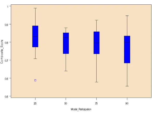
For our main hypothesis, knowledge sharing, we initially assumed that the most relevant and

meaningful results would be drawn from groups that were diligent in working as either solo or paired

programmers. To test this assumption, we used question 10. Question 10 asked each individual to

estimate how well he or she followed their assigned programming model which we refer to as model

participation (MP). The choices for MP were in the form of percentages, signifying how much of the

time a developer programmed using the assigned model; the choices were 25%, 50%, 75% or 90%.

Our assumption meant MP would be important in filtering out groups failing to follow their assigned

programming model closely enough. Contrary to our assumption, we found no correlation between

an individual’s MP and their composite quiz score (as will be discussed in Section 4.1.5) for either

paired programmers (rs = -.08, p = 0.55) or solo programmers (rs = -.25, p = 0.18). Figure 1 illustrates

this using a box and whisker plot of composite quiz score for each of the four possible levels of MP

for all individuals. The same plots for each group (pairs and soloists) look very similar. Due to the

lack of correlation we rejected our assumption and accepted all individuals regardless of MP.

We removed five teams due to incorrect administration of the post-project quiz. Due to

miscommunication with the teaching assistant, these teams were allowed to reference their project

deliverables to answer the quiz questions. Another three individuals were also removed because they

also used project deliverables to complete the quiz. We also completely excluded two more groups

after reading their team retrospective. In the retrospective the teams discussed whether they used

paired or solo development. We rejected teams whose retrospective clearly suggested they didn’t use

their assigned model at all. For example, one PP team writes: “…we switched to solo

programming….I mainly worked on my parts individually…we did a lot of individual programming.”

This response eliminated this team despite their claim they spent 75% of their time using CP. Finally,

since completing the quiz was voluntary, we had some individuals who did not complete the quiz and

(23)

Figure 1: Box plot of composite quiz score by model participation

For the time response, we used question 2, the accuracy of their self-reported time to filter teams

who poorly reported their time data via the Bryce tool. We calculated the average time reporting

accuracy within each group and only accepted groups whose average accuracy was greater than or

equal to 50%, with a group standard deviation of less than 20%.

For implementation quality, the only exclusion of groups was due to lack of data. Quality scores

for one lab section were not available. The data were not available because a teaching assistant

recorded only the final student scores on the project, not the quality scores computed from the test

cases. Table 4 lists the initial and final sample sizes for each major response.

Table 4: Initial and Final Sample Sizes Grouping Initial Sample

Size

Knowledge Sharing Final Sample Size

Quality Final Sample Size

Time Final Sample Size >=50%, <20% Co-located Pairs 61 (15 groups) 38 (10 groups) 14 groups 9 groups

Distributed Pairs 29 (7 groups) 19 (6 groups) 5 groups 4 groups Pairing (Total) 90 (22 groups) 57 (16 groups) 19 groups 13 groups Solo 50 (12 groups) 32 (9 groups) 10 groups 7 groups Total 140 (34 groups) 89 (25 groups) 29 groups 20 groups

(24)

For all quantitative measures, we analyzed if there is a statistically significant difference between

the pair programming and solo programming groups. To accomplish this, we employ a variety of

statistical tests as appropriate. For all comparisons, we considered differences statistically significant

if p <= 0.05. Since we were interested in the difference between paired and solo groups we combined

the results from the distributed and co-located pairs into a single group for all results and analyses that

follow.

4.1 Knowledge Sharing

In our analysis of knowledge sharing, we examine the following hypotheses:

H0,1: The method of programming (solo, paired) and knowledge about project are statistically

independent at the 0.05 level.

dependent at the 0.05 level.

We are presenting this section in a bottom up fashion; we analyse each individual question on the

quiz first, and finally present a cumulative quiz score. We will relate this to the notion of depth

versus breadth of knowledge in the discussion.

4.1.1. Graph

The first question of interest for the knowledge sharing analysis is question 1, “Graph.” Students

were required to draw a directed graph of the major web pages used in their implementation. To

grade this question, we manually examined each group’s web application and drew up our own

version of the directed graph. When necessary, we also used their source files to make the graph. We

compared our correct answer to their answer, making several counts:

• Total number of nodes (N) in our answer, the total number of nodes in their answer (n), and

the total number of correctnodes (cn) in their answer; and

• Total number of links (l) they drew and the total number of correct links (cl) they drew.

We deemed a node correct if its name or description were sufficiently close to the actual name or the

(25)

connected or indirectly connected where the nodes in-between were not pictured on the graph. We

did not attempt to determine the total number of correct links in their entire web application due to the

difficulty in accurately and fairly determining every possible link in each implementation.

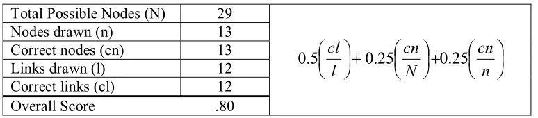
Using these counts, we produced several ratios; correct nodes to total nodes (cn/N), correct nodes

to the number of nodes they drew (cn/n), and correct links to the number of links they drew (cl/l). We

took this result and averaged it with the ratio of correct links (cl/l). Table 5 presents a sample

calculation. In this example, the overall score of 0.8 is a result of the individual drawing about 50%

of the total graph, where everything they drew was 100% was correct.

Table 5: Example Calculation of Graph Score Total Possible Nodes (N) 29

Nodes drawn (n) 13 Correct nodes (cn) 13 Links drawn (l) 12 Correct links (cl) 12

Overall Score .80













+













+













n

cn

N

cn

l

cl

25 .

0

25 .

0

5 .

0

For question 1, Graph, descriptive statistics are presented in Table 6 and a box plot is shown in

Figure 2. The Shapiro-Wilk3_{test for normality suggested the data were not normal for either pairs}

(W = 0.88, p < .0001) or soloists (W = 0.63, p < .0001). For this reason, we performed the Wilcoxon

rank sums test, the nonparametric version of the t-test. Performance was almost equal, soloists

performed slightly better (Mdn. = 0.83) than pairing teams (Mdn. = .82). The difference was not

significant, z = 0.15, p = 0.88.

Table 6: Descriptive statistics for Graph

Style N Mean Median Std. Dev.

PP 57 0.77 0.82 0.14

SO 32 0.75 0.83 0.22

(26)

Figure 2: Box plot for Graph

4.1.2 Schema

The dynamic content of each team’s web application utilized a relational database (MySQL). For

question 2, Schema, we had the developer diagram the database tables and fields. To find the correct

answer, we exported each team’s database tables and used Microsoft Access to produce a diagram of

the actual database schema. We compared the Access-generated diagram to developer’s response on

the quiz. We made several counts:

• The number of tables and fields they drew (t and f respectively) on the quiz

• The number of correct tables (ct) and correct fields (cf) on the quiz; and

• The number of tables and fields in their actual schemas (T and F respectively)

We took similar ratios as before with both tables and fields (ct/t, ct/T, cf/f, cf/F) and computed a

weighted average of these ratios, as shown in

Table 7. We took this approach so we could discriminate and penalize wrong answers more

severely than incomplete answers. A sample calculation is presented in

(27)

Table 7: Example Calculation of Schema Score Total Actual Tables (T) 8

Total Actual Fields (F) 58 Total tables they drew (t) 9 Total fields they drew (f) 37 Correct Tables (ct) 7 Correct Fields (cf) 19 Overall Score: .62













+













+













+













f

cf

F

cf

t

ct

T

ct

25 .

0

25 .

0

25 .

0

25 .

0

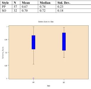
Descriptive statistics for Schema are presented in Table 8 and a box plot is shown in Figure 3.

The responses were non-normal in the paired group (W = 0.91, p = 0.0004) and across both groups

(W = 0.94, p = .0007) but were more normal in the solo group (W = 0.95, p = .17). Due to overall

non-normality, we again used the Wilcoxon rank sums test. Pairs performed slightly better (Mdn. =

0.74) than soloists (Mdn. = 0.72). The difference was not significant, z = 0.12, p = 0.90.

Table 8: Descriptive statistics for Schema

PP 57 0.67 0.74 0.23

SO 32 0.70 0.72 0.18

(28)

4.1.3 Extend

“Extend,” question 5, asked the student to rate on a 1-5 scale how difficult they thought it would

be for their implementation to be extended slightly to implement a new requirement. The answers

formed a 1-5 Likert scale of difficulty where each answer gave a generic description ranging from

“no changes” to “very difficult.” To increase understanding of each answer and to make the answer

more concrete, we included with each answer a description of what that level of difficulty might

entail. To score this question, we studied each group’s implementation and produced what we

considered the right answer. We then compared our answer to the developer’s and found the absolute

difference between the two. The resulting data are ordinal, suggesting the Wilcoxon Rank Sums test.

Soloists (Mdn = 1.0) did not perform significantly different from paired teams (Mdn = 1.0) on

Extend, z = -.76, p = 0.45. Descriptive statistics for Extend are found in Table 9.

Table 9: Descriptive statistics for Extend

PP 57 0.82 1.0 0.68

SO 32 0.75 1.0 0.84

4.1.4 Technology Use

We asked a related set of three questions intended to measure knowledge sharing directly and

knowledge of the implementation. We picked three specific technologies or techniques that were

likely to be used by some of the groups. These technologies, JavaBeans, cookies, and prepared

statements, were specific and germane to what the teams were trying to accomplish with their

implementation. We asked (1) how much they knew about the technology; (2) where they learned

about the technology; and (3) whether their group used the technology in the project. We asked each

question three times, once for each of the three technologies.

The questions regarding how a technology was learned will be considered later, as these are not

directly testing knowledge of the project. With respect to knowledge, we now consider the question:

(29)

refer to this question as “Technology Use.” We determined the correct answer by searching through

each team’s implementations for keywords that must exist if they used a particular technology. We

added up the total number wrong for each individual (max = 3) and compared the two groups. These

data are ordinal since getting none wrong is better than getting one wrong and so on. The data are not

ratio because we cannot reasonably state that someone who got one wrong knows twice as much as

one who gets two wrong. Again, since the data are ordinal we used the Wilcoxon Rank Sums test.

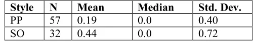
Pair programmers did slightly better (M = 0.19, SD = 0.40) than soloists (M = 0.44, SD = 0.72) but

without statistical significance, z = 1.51, p = 0.13. Table 10 presents relevant descriptive statistics for

Technology Use.

Table 10: Descriptive statistics for Technology Use

PP 57 0.19 0.0 0.40

SO 32 0.44 0.0 0.72

4.1.5 Composite Quiz Score

As mentioned earlier, we are presenting the knowledge sharing results in a bottom up fashion.

We now consider a composite quiz score that combines the previous four questions into a single

number. This number represents the average project knowledge of each individual. To compute this

average, we first converted Extend and Technology Use to a 0-1 scale. This was accomplished by

subtracting the raw response from the maximum possible value for that response (4 for Extend, 3 for

Technology Use) and then dividing the result by the maximum value for the response. The terms

involving Extend and Technology Use in

Table 11

should clarify this calculation. To calculate the composite knowledge score, we averaged the transformed scores for Extend and Technology with the

scores from Graph and Schema . The formula and an example calculation are in

Table 11

.

Table 11: Sample calculation of composite score Graph 0.91 Schema 0.92 Extend 1

(

)

(

)

_      − +       − + + 3 3 25 . 0 4 4 25 . 0 ) ( 25 . 0 ) ( 25 .

(30)

Technology Use 2 Composite Score 0.73

Before analyzing these data, we found a strong positive correlation between an individual’s RAS

(the pre-grouping score, as outlined in Section 3) and the individual’s composite score. After

dropping two outliers whose RAS was less than 20, we found a strong correlation across groups (r =

0.48, p < .0001) and within each group for pairs (r = 0.55, p < .0001) and soloists (r = 0.39, p =

0.033). Since we were looking for an effect of programming style on composite score, we needed to

adjust the response by the covariate (RAS) before comparing composite scores between groups. The

appropriate analysis is the Analysis of Covariance (ANCOVA) where RAS is the covariate. Using

this analysis we found that RAS was significantly related to the composite score, F (1, 84) = 27.96, p

< .0001, suggesting that higher RAS scores lead to higher composite scores. Figure 4 illustrates the

positive association between RAS and composite score for both PP and SO programming models.

After controlling for the covariate RAS, the main effect of programming style on composite score

was weakly significant, F (1, 84) = 1.18, p = .068. Furthermore, the difference indicated the

composite score for paired programmers was slightly higher (Madj = 0.80, SEadj = 0.011) than solo

programmers (Madj = 0.76, SEadj = 0.015).

Table

12

provides descriptive statistics for composite, including both unadjusted and adjusted means.

Table 12: Descriptive statistics for Composite

Style N Mean Std. Dev. Adjusted Mean Adjusted Std. Err.

PP 57 0.79 .0939 0.80 .011

(31)

Figure 4: RAS vs. Composite score

To conclude, we return to our original hypothesis regarding knowledge sharing (Hypothesis 1),

stating that paired programmers would exhibit a higher level of knowledge sharing than solo

programmers. Using our post-project quiz, we have shown no statistical difference in groups when

considering each question individually. However, when the results are combined into a composite

score, representing the average knowledge level of the developer, we have shown weakly significant

evidence suggesting pairs may have a higher level of post-project knowledge than soloists (p < .068).

Statistically, we must fail to reject the null hypothesis:

4.1.6 Methods of Learning

The previous questions have attempted to indirectly measure knowledge sharing by directly

measuring post-project knowledge each individual possessed regarding their team’s project. We also

(32)

know about each of the three target technologies mentioned earlier (JavaBeans, prepared statements,

and cookies). We were interested in instances where individuals learned about a technology from a

team member versus when they learned the technology on their own. Since the data were somewhat

sparse, we recoded the responses. We recoded them such that the results were converted from how

many technologies (Max. = 3) did you learn (on your own / from a teammate) to: did you learn any of

the three technologies (on your own / from a teammate). The results are presented in Table 13 and

Table 14. Each row represents a programming style and each column provides a count of the number

of individuals falling into the category defined by the column heading. For example, in

Table 13

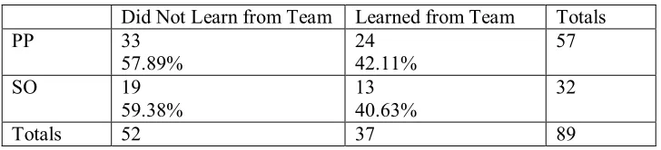
, 38 of 57 pair programmers did not learn any technologies on their own while 19 of 57 did, representing

67% and 33% of pair programmers respectively. A chi-square test of independence was performed to

examine the relation between programming model and how new technologies were learned. The

relationship between programming model and learning a technology on your own was not significant

Χ2_{(89) = 0.34, p = 0.56. Likewise the relationship between programming model and learning}

technologies from a team member was also not significant Χ2_{(89) = 0.0, p = 1.0. In contrast to the}

questions that produced the composite quiz score above; these two results directly measure

knowledge sharing. These results do no allow us to reject the null hypothesis:

Table 13: Learned on Own Contingency Table

Did Not Learn on Own Learned on Own Totals PP 38

66.67%

19 33.33%

57

SO 24 75.00%

8 25.00%

32

(33)

Table 14: Learned from Team Contingency Table

Did Not Learn from Team Learned from Team Totals PP 33

57.89%

24 42.11%

57

SO 19 59.38%

13 40.63%

32

Totals 52 37 89

4.2: Implementation Time

Turning our attention to hypothesis 2, we now examine whether programming style had an effect

the time necessary to complete the project. Specifically, we state our hypothesis as:

H0,2: The method of programming (solo, paired) and implementation time are statistically

H1,2: The method of programming (solo, paired) and implementation time are statistically

dependent at the 0.05 level.

During the project, each developer recorded and reported his or her development time via the

Bryce tool. Unfortunately, developers were less than cooperative using the self-reporting mechanism.

As mentioned above, we used question 2 on the post-project quiz to drop the least accurate groups

with respect to time reporting. We accepted groups with a time reporting accuracy within 50% of

actual and where group’s standard deviation of accuracy was less than or equal to 20%. Twenty

groups out of the original 34 remained and were analyzed for implementation time. Table 15

provides a summary of the time reporting accuracy reported by all individuals on the quiz.

Table 15: Reported Time accuracy

Programming Style Average Time Accuracy Std. Deviation of Accuracy

PP 66.86 % 11.66

SO 62.11 % 15.50

We normalized each group’s total effort by the number individuals in the group. According to

the Shapiro-Wilk test the data were non-normal, (W = 0.88, p = .016), and we performed the

(34)

(Mdn. = 11.56) and the difference was weakly significant, z = -1.66, p = 0.063. Since we found

earlier that RAS was strongly positively correlated with composite score, as reported in section 4.1.5,

we explored whether implementation time may be related to average RAS, but we could find no such

correlation. Table 16 provides descriptive statistics for implementation time while Figure 5 shows a

box plot of effort per person vs. programming style. Although these results offer weak statistical

evidence suggesting there may be a difference in implementation time, formally we must fail to reject

the null hypothesis:

H0,2,: The method of programming (solo, paired) and implementation time are statistically

Figure 5: Box plot for Implementation Time

Table 16: Descriptive statistics for Implementation Time

Style N Median Mean Std. Dev.

PP 13 18.75 19.48 11.10

SO 7 10.75 11.56 6.46

4.3: Implementation Quality

Finally, we address hypothesis 3, that pair programmers would produce a higher quality product

(35)

H0,3: The method of programming (solo, paired) and implementation quality are statistically

H1,3: The method of programming (solo, paired) and implementation quality are

statistically dependent at the 0.05 level.

To measure implementation quality, we applied a set of test cases to the final project. These tests

were a set of 40 black-box tests, of which students were given access to 31 of the 40 tests. Providing

31 of 40 black-box tests may partially explain this lack of significant difference between the two

groups. We attempted to get a breakdown of results by the 31 known to nine unknown tests to

examine whether the results might be different for the nine blind tests. Unfortunately, the teaching

assistants collected only overall scores so these data were not available.

Soloists had slightly higher quality scores (Mdn. = 0.96) than pair programmers (Mdn. = 0.95).

According to the Wilcoxon rank sums test the difference was not significant, z = -.07, p = 0.94.

Summary statistics may be found in

Table 17

and a box plot is available in

Figure 6

. These results offer no statistical evidence that PP had an effect on product quality; we therefore fail to reject the

null hypothesis:

H0,3:

The method of programming (solo, paired) and implementation quality are

statistically independent at the 0.05 level

Table 17: Summary statistics for Quality

PP 19 0.94 0.95 0.071

(36)

Figure 6: Box plot for Quality

Table 18 provides a summary of all results presented in this section. It presents the results for

each response as measured for both groups. The last column presents the result of the appropriate

statistical test for each response, and the corresponding p-value.

Table 18: Quantitative Results Summary

Examination Model Participation

Mean / Median Standard Deviation

Statistical Result

Knowledge Sharing

Pairs 0.77 / 0.82 0.14

Graph

Soloists 0.75 / 0.83 0.22

z = 0.15, p = 0.88

Pairs 0.67 / 0.74 0.23

Schema

Soloists 0.70 / 0.72 0.18

z = 0.12, p = 0.90

Pairs 0.82 / 1.0 0.68

Extend

Soloists 0.75 / 1.0 0.84

z = -.76, p = 0.45

Pairs 0.19 / 0.0 0.40

Technology Use

Soloists 0.44 / 0.0 0.72

z = 1.51, p = 0.13

Pairs 0.804_0.0115

Composite Score

Soloists 0.764_0.0155 F (1,84) = 1.18, p = 0.068

Learned on Own Χ2_{(89) = 0.34, p = 0.56}

Learned from Team Χ2_{(89) = 0.0, p = 1.0}

Time and Quality

Time Medium 19.48 / 18.75 11.10

4_{Mean adjusted for RAS}

(37)

High 11.56 / 10.75 6.46 z = -1.66, p = 0.063

Medium 0.95 / 0.95 0.071

Quality

High 0.94 / 0.96 0.069

z = -.07, p = 0.94

4.4: Discussion

Returning our attention to the knowledge-sharing hypothesis, we would like to explore the results

of the quiz in more depth. We will discuss in depth the different questions asked on the quiz and how

they relate to our definition of knowledge. As mentioned earlier, we recognize two types of

knowledge, explicit and tacit. Explicit knowledge is knowledge that can easily be recorded and

therefore easily shared. Tacit knowledge, in contrast, is both difficult to record and difficult to share.

We have attempted to compare how two very different software development methodologies effect

knowledge sharing. Since knowledge is divided into these two predominant forms we point our

discussion in the direction of understanding in terms of these two types.

Questions Graph and Schema were measures of explicit knowledge. The information necessary

to answer these questions could be gathered from the product deliverable without any contextual

information or tacit knowledge. With respect to these two questions, we observed a pattern in the

answers to Graph not present or possible with Schema. We found that developers with superficial

knowledge of the problem and their team’s implementation could get an inflated score without

necessarily demonstrating knowledge of their actual system. That is, if the project had a user

requirement such as “take survey,” and a student knew his or her team had all the major links on a

main menu page, he or she could correctly guess and draw a link between a “main menu” node and a

“take survey” node. Therefore, a high score on graph did not necessarily mean an individual actually

had a working knowledge of the system. For this reason, and the fact that Graph was more

subjective, we consider Schema to be a slightly better measure of explicit knowledge.

While Schema and Graph measure explicit knowledge, Extend and Errors attempt to measure

developer’s tacit knowledge. A correct answer for Extend required knowledge about how the entire

system was put together, the overriding principles the group used, and the experience of putting it

(38)

be to extend their implementation given a specific new feature outlined in the question. The strength

of the question is that it requires both broad and deep knowledge about the implementation, where

most of the knowledge is tacit. Its major drawback is that the answer is subjective, both on the part of

the developer and the part of the evaluator. We had to study the implementations carefully and make

our subjective estimate of the difficulty and then compare that to the developers’ subjective estimate

of the difficulty.

We also claim that Technology Use, which requires knowledge of the specific technologies used,

is somewhat tacit in nature, because groups did not explicitly record which technologies they used; it

was implicit in their implementation. Arguably, those teams that shared more experience and more

tacit knowledge about the problem and their solution would have an easier time recalling which

technologies the team used, even if the individual had no part in the actual technology. The results of

these questions suggest that pairs were slightly better equipped to answer questions requiring tacit

knowledge than soloists. Overall, these results were not statistically significant, but the pattern of

success for pairs with respect to tacit knowledge argues that there may be some advantage to pairing

as it applies to tacit knowledge. As mentioned earlier, we consider PP to be a CoP-like environment

that acts as an efficient mechanism of tacit knowledge transport between individuals.

5. Summary and Future Work

In this study we were interested in how programming style, either paired or solo affected three

things: knowledge sharing, implementation time, and implementation quality. Summary results for

each hypothesis is presented in Table 19. Of these three, we were most interested in knowledge

sharing. To assess the difference in knowledge sharing, we made up a post-project quiz asking

pointed questions about the product their team delivered. These questions required knowledge of the

project, and we claim the level of knowledge exhibited on the quiz is related to how much knowledge

was shared across the team throughout the project. From this quiz, we studied the differences in

(39)

any significant difference between soloists and paired teams for any individual question. We did find

weak statistical evidence suggesting paired developers had slightly higher composite quiz scores.

This finding only emerged after we controlled for each individual’s RAS, or pre-grouping score. The

RAS was a combination of current grade in the course and a score based on their experience with

technologies that would be important during the course of the project. RAS was positively and

significantly correlated with the composite score on the quiz.

Table 19: Summary of findings by hypothesis Hypothesis Findings

H1: Pairs will exhibit more knowledge sharing

No evidence on individual questions. Weakly significant evidence found supporting hypothesis for the composite quiz score.

H2: Pairs will have comparable or shorter development time

Weakly significant results suggesting pairs took longer than soloists.

H3: Pairs will produce a higher quality product

No significant evidence suggesting a difference in product quality

We then considered whether programming style affected a difference the time necessary to

implement the web application. This comparison resulted in an unexpected finding. There was weak

statistical evidence suggesting pairs took almost twice as long to develop the product. This refutes

earlier findings, both anecdotal and statistical, such as those in [5, 7, 8][9][13]. One possible

explanation is that by combining distributed and co-located pairs we introduced distributed pairing

overhead not seen before in co-located pairing. This does not seem to be the case as the results from

the distributed groups were quite similar to the results from co-located groups. Another explanation

may stem from significant differences in time reporting accuracy between the two groups. We looked

for these differences in the reporting accuracies and reporting accuracy standard deviations within

paired and solo groups and could find nothing significant. The best explanation may stem from the

perceived and actual difficulty in using the Bryce tool to record time spent. For instance, in their

An Empirical Study of the Tacit Knowledge Management Potential of Pair Programming

ABSTRACT

An

Empirical Study of the Tacit Knowledge Management

Potential of Pair Programming

by

Dylan Garrett Wilson

A thesis submitted to the Graduate Faculty of

North Carolina State University

in partial fulfillment of the

requirements for the Degree of

Master of Science

COMPUTER SCIENCE

Raleigh

2004

APPROVED BY:

_________________________ _________________________

__________________________

Chair of Advisory Committee

Biography

Table of Contents

LIST OF TABLES

...V

LIST OF FIGURES

... VI

1. INTRODUCTION ...1

2. BACKGROUND AND RELATED WORK ...2

2.1 P

P

...2

2.2 K

M

...4

2.3 K

M

P

P

...8

3. EXPERIMENT...9

3.1. E

D

...9

3.2. E

L

...13

4. QUANTITATIVE RESULTS AND ANALYSIS...14

4.1 K

S

...17

4.1.1. G

...17

4.1.2 S

...19

4.1.3 E

...21

4.1.4 T

U

...21

4.1.5 C

Q

S

...22

4.1.6 M

L

...24

4.2: I

T

...26

4.3: I

Q

...27

5. SUMMARY AND FUTURE WORK...31

6. APPENDICES

...37

6.1. T

P

P

F

...38

List Of Tables

_ _