Dynamic model of a simple supported RC rectangular plate for spreadsheet application - Part II: Motion in elasto-plastic domain

(1)

20th International Conference on Structural Mechanics in Reactor Technology (SMiRT 20) Espoo, Finland, August 9-14, 2009 SMiRT 20-Division III, Paper 1646

Dynamic model of a simple supported RC rectangular plate for spreadsheet

application – Part II: Motion in elasto-plastic domain

Jean-Mathieu Rambach

Institut de Radioprotection et de Sûreté Nucléaire (IRSN), Fontenay-aux-Roses, France, e-mail: [email protected]

Keywords: dynamic motion, rectangular plate, reinforced concrete, impact, elasto-plastic domain, spreadsheet application, yield surface, hinge.

1 ABSTRACT

This paper is intended to provide civil engineers with a simple modeling tool to be run on current spreadsheet code. Such a tool allows performing the resolution of the dynamic motion of an elasto-plastic simply supported thin rectangular plate, made of reinforced concrete, when submitted to impact loading.

The rupture by flexion is characterized by a criterion of Johansen’s type with correction factors to avoid singularities and for keeping law consistency. With the limiting bending moments in x and y

directions for face I and face II,

M

Ix, I y

M

,

II x

M

and

M

IIy, the criterion is expressed by:

! ! !

" ! ! !

# $

=

% %

+ =

=

% %

+ =

0 ) M M ).( M M ( -k k M ) M ( f or

0 ) M M ).( M M ( -k k M ) M ( f

y II y x II x 2 1 2 2 2 xy II

y I y x I x 2 1 2 2 2 xy I

r r

with

(

)

(

)(

)

!

"

!

#

$

%

&

%

+

%

=

<

)

M

).(

M

(

k

0 and

M

.

M

.

4 M

M

k

0

II y I y II x I x 1

2

II y I y II x I x

II y I y II x I x 2

2

When

f

I

(

M

r

)

or

f

II

(

M

r

)

>0, a correction

!

M

r

is to be applied to the bending moment

vector

M

r

=

t

(Mx,

My,

Mxy)

whose value shall be considered as the trial value. The plastic curvature tensor increment is deduced from the consumption of the incremental elastic energy into energy dissipation due to plastic deformation, the plastic displacement is computed by double integration of the curvatures.

The motion of the plate is based on:

The computation is performed by finite differences on displacements decomposed on the modes space. The plate discretization into 30x30 elements gives sufficient accuracy for pre-sizing RC plates against impact loading and for checking results from more sophisticated non linear code.

2 INTRODUCTION

This paper deals with the modeling of the dynamic behavior of a rectangular reinforced concrete slab, which is simply supported and submitted to a variable loading. It complements the part I [Rambach, 2009] paper that was restricted to the elastic domain: in this paper an elasto-plastic law is introduced. The proposed yield limit for the elastic domain is of Johansen’s type with a little adaptation in order to be locally and globally consistent and in order to get a yielding surface without singularities, as “smooth” as possible. The classical method of plastic correction by cutting plane is presented and adapted to the spreadsheet code possibilities, for static case then for dynamic case. An application is proposed in order to demonstrate the efficiency of the method.

0 Q y? ?My y

x. ?Mxy 2. x? ?Mx )

t w ù. î. 2. t? ?w .( .h

ñ ! =

" " + " " " + " " + " " +

(2)

3 THEORETICAL BACKGROUND

3.1 Fundamental equation of motion of a thin plate

The fundamental equation of motion o a thin plate is expressed by:

0 Q y? ?My y x. ?Mxy 2. x? ?Mx ) t w ù. î. 2. t? ?w .( .h ñ ! = " " + " " " + " " + " " + " " ₍₁₎

with usual notation:

ρ: mass to volume ratio of the constitutive material of the plate, ξ: critical damping ratio,

ω: 1st mode pulsation h: plate thickness supposed constant

Mx, My and Mxy: components of the bending moment tensor Q=Q(x,y,t): loading distribution

The expression (1) can be considered as the balance of the loading Q by the sum of the inertial force density (part involving

t? ?w

!

! _{), the viscosity force density (part involving}

t w

!

! _{), and the resisting force density}

exerted by the structure

y? ?My y x. ?Mxy 2. x? ?Mx Fs ! ! + ! ! ! + ! !

= (1’)

For a simply supported rectangular plate in the elastic domain, a method of resolution of this equation is proposed in [Rambach, 2009], by recurrence and modal decomposition. The propagation of the solution with time is made, in the modal space, according to the following set of 2 equations:

! ! " ! ! # $ + % + & + % ' + = % + + + ' % & ' % ' ' = % + + + + + + 2 Q Q .h 4. Ät? V . D . t ).Fs D .h 4. Ät? î.ù.Ät (1 ).Fs D .h 4. Ät? î.ù.Ät (1 ) 2 Q Q Fs ( ñ.h t ).V D .h 4. Ät? î.ù.Ät (1 ).V D .h 4. Ät? î.ù.Ät (1 t mn Ät t mn t mn mn t mn mn Ät t mn mn t mn Ät t mn t mn t mn mn Ät t mn mn ( ( ( (

( ₍₂₎

2 2 2 mn ) b n.! ( ) a m.! ( D. D

with _!

" # $ % & ₊ =

It is necessary to come back from the modal space into the physical space, at each time step, in order to get the successive values of the displacement and bending moments.

3.2 Bending moment - Curvature law in elasto-plastic domain

For a beam, the bending moment – curvature law is simply expressed, for an isotropic elastic - perfectly plastic material, by M=EIχ (χ being the curvature and EI being the rigidity) for χ≤ Mpl/EI and M=Mpl for χ ≥ Mpl/EI, Mpl being the limit bending moment.

For a plate, the bending moment – curvature law in the elasto-plastic domain is less easily expressed, owing to the fact that it involves relation between bending moment tensor and curvature tensor.

The bending moment – curvature law between the tensors components in elastic domain is as follows:

!! " # $$ % & ' ' + ' ' = y? ?w í. x? ?w D.

Mx , _!!

" # $$ % & ' ' + ' ' = x? ?w í. y? ?w D. My and y x. ?w í). D.(1 Mxy ! ! ! "

= , (3)

with í?) 12.(1 E.h D 3 !

= the plate stiffness (E: Young’s modulus and ν : Poisson’s ratio). (4)

In the plastic domain, the limitation of the bending moment components is generally expressed by a yield surface, in the bending moment space, on which the point (Mx, My, Mxy) representative of the stress state will be located. A first attempt has been proposed by [Nahas, 1983] in SMiRT 7 Proceedings.

4 YIELD SURFACE

(3)

capacity into resisting bending moment: there are 4 resisting moments that can be called

M ,

Ix I y

M ,

M

IIx

and

M

IIy, the index x (y) corresponds to the direction of the acting rebars, the exponent I or II corresponds to

the conventional sign for the bending moment, I (II) put in tension the lower (upper) face.

The criterion is said of Johansen’s type when the relation between the bending moments of the slab Mx, My and Mxy and the resisting moments at plasticity is:

(5b)

0 )

M

).(

M

(

-M

)

M

(

f

or

(5a)

0 )

M

).(

M

(

-

M

)

M

(

f

y II y x II x 2 xy II

y I y x I x 2 xy I

!

"

!!

#

$

=

%

=

%

=

With

M

=

t

(

Mx,

My,

Mxy)

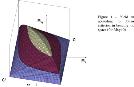
In the (Mx, My, Mxy) space, the Johansen criterion is represented by two coaxial and opposed cones, see Figure 1 below representing the surface for Mxy ≥ 0.

The yield surface envelops the elastic domain: when the representative point (Mx, My, Mxy) of the stress state is strictly inside the yield surface (and not located on the surface), the representative point is said in the elastic domain, when the point is on the yield surface, the point is said in the plastic domain. The yield surface is supposed constant (there is no hardening nor softening: the plasticity is supposed perfect).

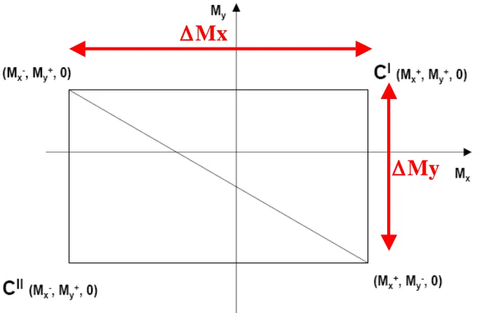
The projection of (Mx, My, Mxy) on the (Mx, My) plane shall be located inside a rectangle whose

corners are defined by the limiting bending moments:

M

Ix, I y

M

,

M

IIx_and II y

M

i.e. (

M

Ix, I y

M

), (

M

Iy, II

x

M

), (

M

IIx, II y

M

) and (

M

IIx_, I y

M

), see Figure 2.

(4)

Figure 2 – Projection of the yield surface on the (Mx, My) plane, the projection of the bending moment triplet is located inside the rectangle defined by the cone summits CI and CII.

A criterion of this type has been used by Koechlin in his PhD thesis [Koechlin, 2007], by

taking into account, in addition, the membrane force.

4.2 Modified Johansen’s criterion

Two modifications are introduced with the two following parameters: the first one, k1, for regularization of

the surface in the vicinity of the cone summits and the second one, k2 , for the consistency of the criterion in

its global and local expression.

Regularization

The Johansen’s yield surface has 2 punctual singularities (the summits CI and CII) and a linear singularity (the intersection of the 2 cones). It is convenient to regularize the yield surface near the summits, in order to get a continuous normal in the vicinity of the summit. The coefficient k1 is then introduced and its physical

meaning is discussed below.

Local and global consistency of the criterion

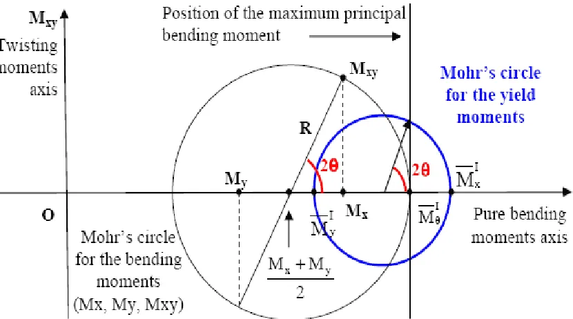
The Johansen’s criterion (5a and 5b) may be considered as expressed under its global form. In Mohr’s representation, the bending moments Mx or My are along the abscissa axis and the twisting moment Mxy along the ordinate axis, and a triplet (Mx, My, Mxy) defines a circle whose centre is on the abscissa axis at

the position

2 ) M

(Mx+ y _{and whose radius is equal to}

4 ) M -(M M R

2 y x 2 xy+

= .

The maximum principal value of the bending moment, M1 is equal to

4 ) M -(M M 2

M

M 2

y x 2 xy y

x+ ₊ ₊ _.

In this representation, the resisting bending moment

M

I_è , for a section whose normal is oriented by the angle θ with respect to x direction, is given by:

è

sin

M

è

cos

M

2 Iy 2

I x I

è

=

!

+

!

The plastic state is reached for the section oriented by θ (defined by the triplet (Mx, My and Mxy)) and I

M

Δ

Mx

(5)

Figure 3 – Mohr’s circle representation of Johansen’s criterion

When the reinforcement is the same on each face of the plate, the bending moments

M

Ix and II x

M

(resp.

M

Iy and II y

M

) are opposed: at the centre of the rectangle, Mx=0 and My=0 and the value of (Mxy)²,

according to Johansen’s criterion, shall be (

M

Ix).( I y

M

) = (

M

IIx) .( II y

M

). The plasticity is reached by the twisting moment Mxy at its extreme value, and the orientation of the rupture line is at 45° with respect to the

principal directions x, y: it means that (Mxy)² shall be equal to [(

M

Ix)+( I y

M

)]²/4 or [(

M

IIx) +( II y

M

)]²/4. This is the reason why the Mxy value has to be corrected by dividing it by the coefficient k2>0 in order to

ensure the consistency of the Johansen’s criterion expressed in its global form and in its local form.

The modified expression of the criterion after regularization and consistency is then as follows:

(6b)

0 )

M

).(

M

(

-k

k

M

)

M

(

f

or

(6a)

0 )

M

).(

M

(

-k

k

M

)

M

(

f

y II y x II x 2 1 2 2 2 xy II

y I y x I x 2 1 2 2 2 xy I

!

"

!

#

$

=

%

+

=

%

+

=

r

(

)

2)

figure

(see

M

ÄMy

and

M

ÄMx

(7)

ÄMy

ÄMx

4 ÄMy

ÄMx

k

0 With

II y I y II

x I x

2 2

2

!

=

!

=

"

+

=

<

It can be checked that k2=1 when I x

M

= -

M

IIx= I y

M

= -

M

IIy_{i.e. when the ratio}ΔMx/ΔMy = 1. When

the ratio ΔMx/ΔMy is comprised between 0.5 and 2, the coefficient k2 is then comprised between 1 and 1.25.

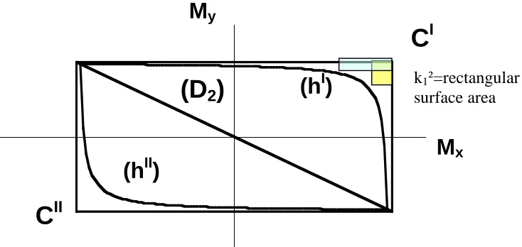
Equations (6a) and (6b) are the equations of the 2-sheeted hyperboloids (HI) and (HII) having for asymptotic surfaces the preceding cones (CI) and (CII). The trace of the hyperboloids (HI) and (HII) on the plane (Mx, My) are the hyperbole branches (hI) and (hII) located inside the rectangle (axb), see Figure 4. The equations of the hyperbole branches are:

0 )

M

).(

M

(

-k

_x Iy _y

I x 2

1

!

=

and

k

-

(

M

).(

M

y

)

0

II y x II x 2

(6)

Geometrically, k₁2 is the expression of the area of the rectangle having for corners (CI) or (CII) and the

current point (Mx, My) of the hyperbole branch (hI) or (hII). In other words, k₁ can be considered as the

side length of the largest square located between the asymptotes and the hyperbole branch: k₁ is then the maximum closest distance of the hyperboloid to the cone surface, it then characterizes the approximation of the cone by the hyperboloid.

The intersection of the hyperboloids (HI) and (HII) occurs along an ellipse located in a plane perpendicular to (Mx, My) plane in (Mx, My, Mxy) space, and whose trace on this plane is the diagonal (D2) other than that (D1) containing the corners CI and CII of the rectangle (axb). It can be demonstrated that the major axis of above ellipse is the part of preceding diagonal comprised between the intersections with the

hyperbole branches, as shown on Figure 4 and whose length is equal

to:

ÄMy

ÄMx

k

1 ÄMy

ÄMx

2 1 2 2

!

"

!

+

; the minor axis is equal to

ÄMy

ÄMx

k

1 )

2 ÄMy

ÄMx

(

2 1

!

"

!

+

. It can be noted that the lower the value of

ÄMy ÄMx

k12

! is, the better

the approximation of the cones by the hyperboloids is. A practical value -2

2 1

10 ÄMy

ÄMx

k

₌

!

is sufficient.

The normals to the hyperboloids are discontinuous when crossing the above ellipse; nevertheless, it can be admitted that the normal for a current point from this ellipse is carried by the intersection of the plane of ellipse with the plane pivoting around diagonal D1 and containing the current point. In other words, the normal to the surface along this ellipse is equal to the half-sum of the normals deduced from each hyperboloid.

The expression of the equation of the yield surface formed by the two intersecting sheets from those two hyperboloids may be simply written in a compact form. The projection of the whole yield surface on the plane (Mx, My) is limited by the two hyperbola branches (hI) and (hII) having for asymptotes the sides of the above-mentioned rectangle and intersecting on diagonal (D2). The position of the current projection point (Mx, My) with respect to diagonal (D2) defines the hyperboloid to which the current stress representative point M on the yield surface belongs.

Let us define ϕ by _II

y I y I x y II x I x II x x

M

-M

M

-M

M

-M

M

-M

+

=

!

_{: the sign of}ϕ characterizes the location of the

projection of the representative point M(Mx, My, Mxy) on the projection of the yield surface on (Mx, My) plane. ϕ>0 means M∈(H1), ϕ <0 means M∈(H2) and ϕ = 0 means M∈(H1) and M∈(H2), i.e. M belongs to the ellipse (E) that seams the hyperboloids (H1) and (H2) sheets, the projection of (E) being diagonal D2.

Let us define Ψ: Ψ=1 when ϕ >0, Ψ=-1 when ϕ <0 and Ψ=0 when ϕ = 0. With this notation, the expression of the yield surface is:

(7)

Figure 4 – Intersection of the hyperboloid sheets with (Mx, My) plane: hyperbole branches (hI) and (hII)

5 INCURSION IN THE PLASTIC DOMAIN

5.1 Bending moment tensor in plastic domain

When f(Mr) <0 the representative bending moment vector

M

r

issued from the origin of the bending moments space is in the elastic domain and when f(Mr) =0, the extremity of the representative vector

M

r

is on the yield surface and therefore in the plastic domain; there is no possibility for a representative vector

M

r

to cross the yield surface, i.e. such as f(Mr) >0.

Let us define the elastic increment vector

Ä

M

r

e

=

t

[Ä

M

e_x

ÄM

e_x

ÄM

_xye

]

of the representative bending

moment vector Mt r

(t : at the time t) during the time increment Δt. Let us define the trial value

M

r

trial :

e t

trial

M Ä M

Mr = r + r . If the trial value t e

trial

M Ä M

Mr = r + r is such that f(Mr trial) >0 (i.e.

M

r

trial outside the

yield surface), there is a coefficient 0 ≤ µ <1 such that f(Mr +ì !ÄMr e) =0 (µ = 0 if M is already on the yield surface, µ ≠1 because f(Mr trial) >0). Let us define M* the point where the elastic increment vector

M

Ä

r

e crosses the yield surface: the normal to the yield surface at the point M* is parallel to

grad

(f(

M

*

))

,

*

M

r

being the representative bending moment vector associated to the point M*.

5.2

Cutting plane method

The cutting plane method is a way to force to the representative point of the bending moment tensor

to rest on the yield surface: a corrective bending moment vector

!Mr p_c must be added to

M

r

trial in order to locate Mr _t₊_Ät =Mr trial +ÄMr _cp on the yield surface, i.e. f(Mr trial +ÄMr p_c)=0

The Hill’s theorem implies that the vector involving the plastic curvature increment

"

!

r

p

shall

be normal to the yield surface of corresponding bending moments, i.e. there is a coefficient

λ

>0

such as

Ä

Ö

ë

grad

(f(

M

))

* p

!

=

r

. Let us assume that the relationship between

ÄMr p_c and

"

!

r

p is of

the same type as the one supposed in elastic domain: ÄMr p_c =#

[ ]

Kp "!rp (

[ ]

Kp is the tangent incremental

elasticity matrix with possibly reduced value,

[ ]

Kp is supposed invertible, the sign – is introduced in order

to mean that the “direction” of ÄMr p_c is opposite to that of

"

!

r

p ).

Owing that

Ä

M

r

e is small with respect to

M

r

trial , it can be demonstrated that the coefficient λ is given by:

M

x

M

y

C

II

C

I

(h

II

)

(h

I

)

(D

2

)

(8)

(9)

))

M

(f(

grad

].

[K

))

M

(f(

grad

)

M

f(

))

M

(f(

grad

].

[K

))

M

(f(

grad

))

M

(f(

grad

ÄM

ì)

-(1

ë

_*

p *

trial

* p

*

* e

• =

•

• !

=

The symbol

• corresponds to the scalar product. The bending moment representative vector

Mr_t₊_Ät

,

after correction and at the end of the time increment

Δ

t, is given by:

[ ]

₍₁₀₎

))

M

(f(

grad

].

[K

))

M

(f(

grad

))

M

(f(

grad

K

)

M

f(

M

Ä

M

_*

p *

* p

trial trial

p c trial

Ät t

• !

"

=

+

=

+

r

The expression (10) shows that the correction

ÄMpc r

is weakly dependent on the tangent incremental elasticity matrix [Kp]: if [Kp] is reduced to the unit matrix, the formula indicates that the representative point

Ät t

M ₊

is obtained as the normal projection on the yield surface of the extremity of the representative

point

M

trial (see Figure 5), ÄMpc r

is parallel to grad(f(M*)) and its norm is equal to f(Mtrial) / grad(f(M*)) .

Figure 5 – Scheme showing the correction to the bending moments on the yield surface

5.3 Structural response force Fs

Once the bending moments are corrected, the structural response force Fs is computed by second

derivation of the bending moments, according to (1’). The obtained value of Fs is to be decomposed

on the modal basis and has to be substituted to the value proposed by equations (2).

5.4 Plastic displacement

The

plastic

curvature

increment

"

!

r

p is not deduced from the preceding relation

))

(f(M

grad

ë

Ö

Ä

r

p

=

!

* , but from the hypothesis of plastic deformations concentrated along hinges: the

curvature increment reaches its maximum value ΔΦ1 in the same principal direction θ where the bending

moment reaches its maximum absolute value M1 (which is also the yield value), whereas in the perpendicular

direction, the curvature increment is nil. According to these assumptions, the vector of curvature plastic

[

]

t

=

(9)

[

1 cos(2

è)

]

2 ÄÖ

ÄÖ

p 1

x

=

!

+

!

,

[

1 cos(2

è)

]

2 ÄÖ

ÄÖ

p 1

y

=

!

"

!

and

sin(2

è)

2 ÄÖ

ÄÖ

p 1

xy

=

!

. (11)

If the direction θ cannot be determined, i.e. when M2 = M1,

and

ÄÖ

0

2 ÄÖ

ÄÖ

pxy

1 p

y p

x

=

The energy dissipation density due to the plastic deformation ΔEp is equal to:

p xy xy p

y y p x x p

ÄÖ M

2 ÄÖ M ÄÖ M

ÄE = ! + ! + ! ! (12)

After some algebraic manipulations, it can be demonstrated that 1 1

p

M

ÄE = #!" . The intensity of the curvature increment ΔΦ1 is obtained by equating the energy dissipation density (due to plastic deformation)

to the difference between the elastic energy density Ee(

M

r

trial ) of the stress state represented by

M

r

trial and the elastic energy density Ee(Mr_t₊_Ät) of the stress state represented by Mr _t₊_Ät, after correction.

The elastic energy density stored in a thin plate (when neglecting shear distortion) is given by:

[

]

[

]

! ! !

" ! ! !

# $

% % % &

+

% %

%

=

% %

+

%

+ +

% %

%

=

moments bending

principal the

being M

and M

, M M 2 M M ) -(1 D 2

1

) M M -M ( ) (1 2 ) M (M ) -(1 D 2

1 )

M ( E

2 1

2 1 2

2 2 1 2

y x 2 xy 2

y x 2

e

'

(13)

Once the plastic curvature increment

"

!

r

pis determined, the plastic displacement increment

!

W

p is computed by direct double integration, according to the definition of the curvature and the limit conditions W=0 all along the 4 edges of the plate. It is thus possible to determine the corrected value of the velocity:

Ät

ÄW

ì

V

p e

t Ät

t+

=

+

!

+

, (14)

W

e

!

being the elastic displacement increment associated to the bending moment increment M

e ! . The value of

V

t+Ät is to be decomposed on the modal basis and to be substituted to the

value proposed by

equations (2).

The displacement Wt+Δt , in physical space, is thus simply obtained by:

Ät

2 V

V

W

t Ät t t Ät t

!

+

=

+

. (15)

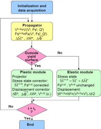
5.5 Practical Algorithm

The following Figure 6 proposes a structure of algorithm allowing the computation of the motion of

a thin plate in elastic and beyond elastic domains.

The module called “propagator” is the module that ensures the progression of the motion: the

recurrence formula allows the computation of the value, in the modal space, of V and Fs at the step

time t+

Δ

t from the knowledge of their value at the time t and of the applied loading value Q. The

values of V and Fs are translated in the physical space by modal summation at each time step, in

order to compute the displacement increment and then the bending moment tensor

Ä

M

r

e

increment.

At each time step, the location of the extremity of the representative vector

Mr trial =Mr _t +ÄMr e

is

tested with respect to the yield surface: if

M

r

trial

is outside the yield surface, the results are processed

by the “plastic module”, if not by the “elastic module”.

The module called “plastic module” is intended to correct the bending moment, to correct the

structural force Fs, to compute the plastic curvature increment, the plastic displacement increment

and then to correct the velocity.

The “elastic module” is intended to compute the displacements, whereas the velocity and the

structural force are unchanged.

(10)

Figure 6 – Diagram showing the algorithm for resolution of the motion of a thin

rectangular plate, in elasto-plastic domain, submitted to a variable loading

6 CONCLUSIONS

The motion of a simply supported elasto-plastic RC plate when submitted to a variable loading can

be simulated on current spreadsheet software. The dominant rupture mode is by flexion. The

accuracy is sufficient to pre-size a RC rectangular plate against impact loading and to check an

order of magnitude of the maximum and of the permanent deflections coming from results of more

sophisticated non linear computation code.

REFERENCES

Rambach, J.-M. Dynamic model of a simple supported RC rectangular plate for spreadsheet application – Part I: Motion in viscous-elastic domain, in SMiRT 20 Proceedings, Espoo, Finland, 9-14 August 2009.

Nahas, G. et al. Application of a global plasticity model to determine the ultimate strength of a reinforced concrete slab, in SMiRT 7 Proceedings, Chicago, Illinois, USA, August 1983.